
Design and Control of a Reconfigurable Robot with Rolling and Flying Locomotion

Abstract
1. Introduction
2. Design of the Reconfigurable Robot
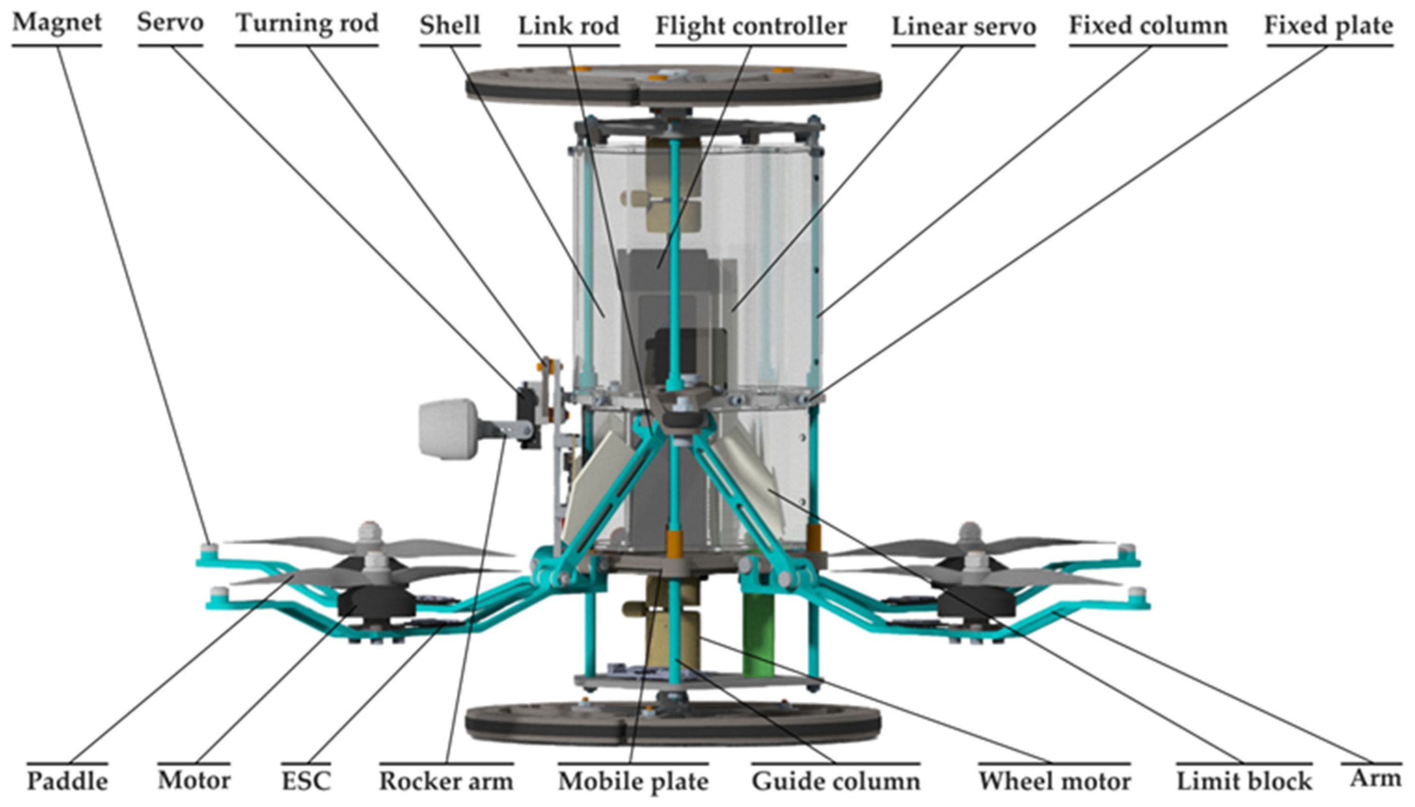
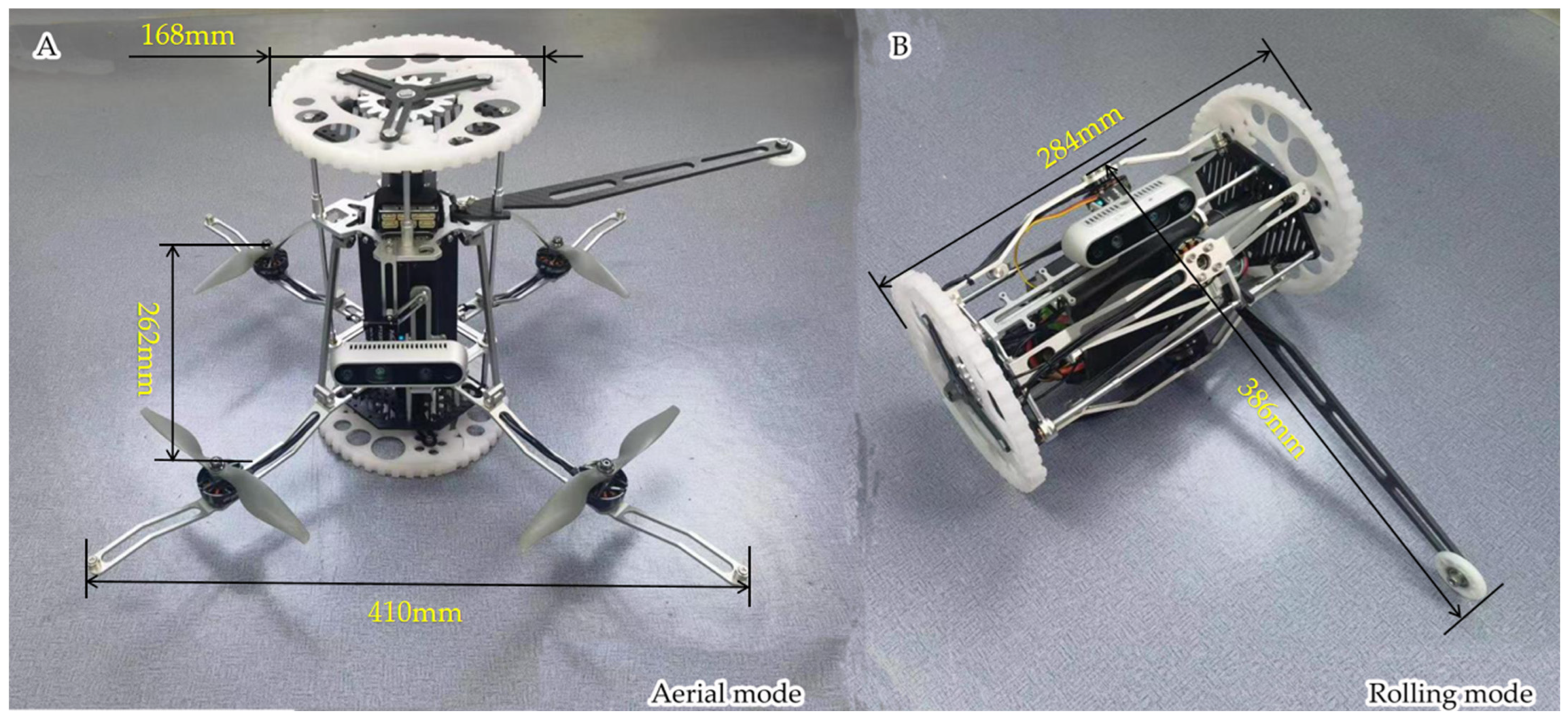
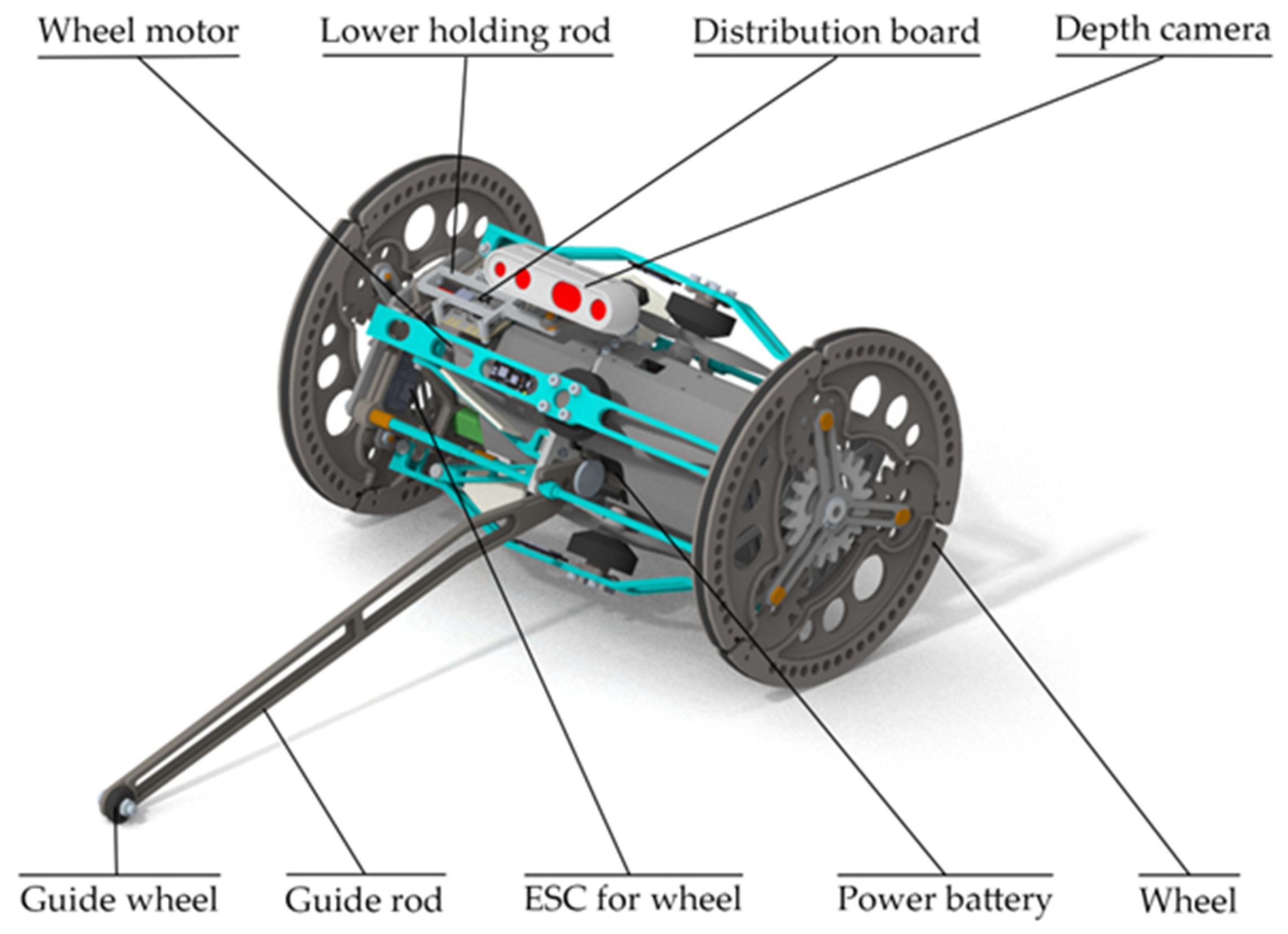
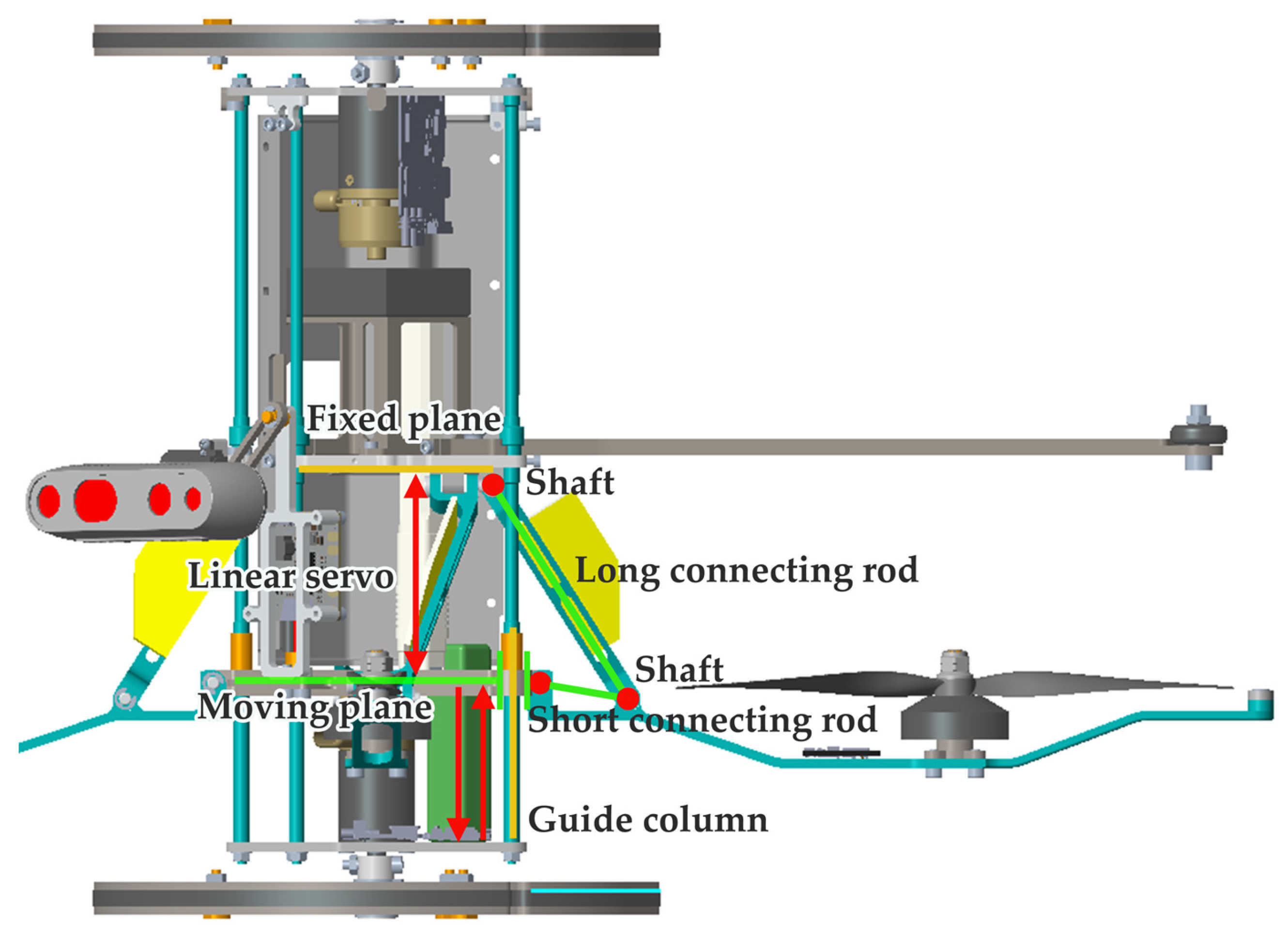
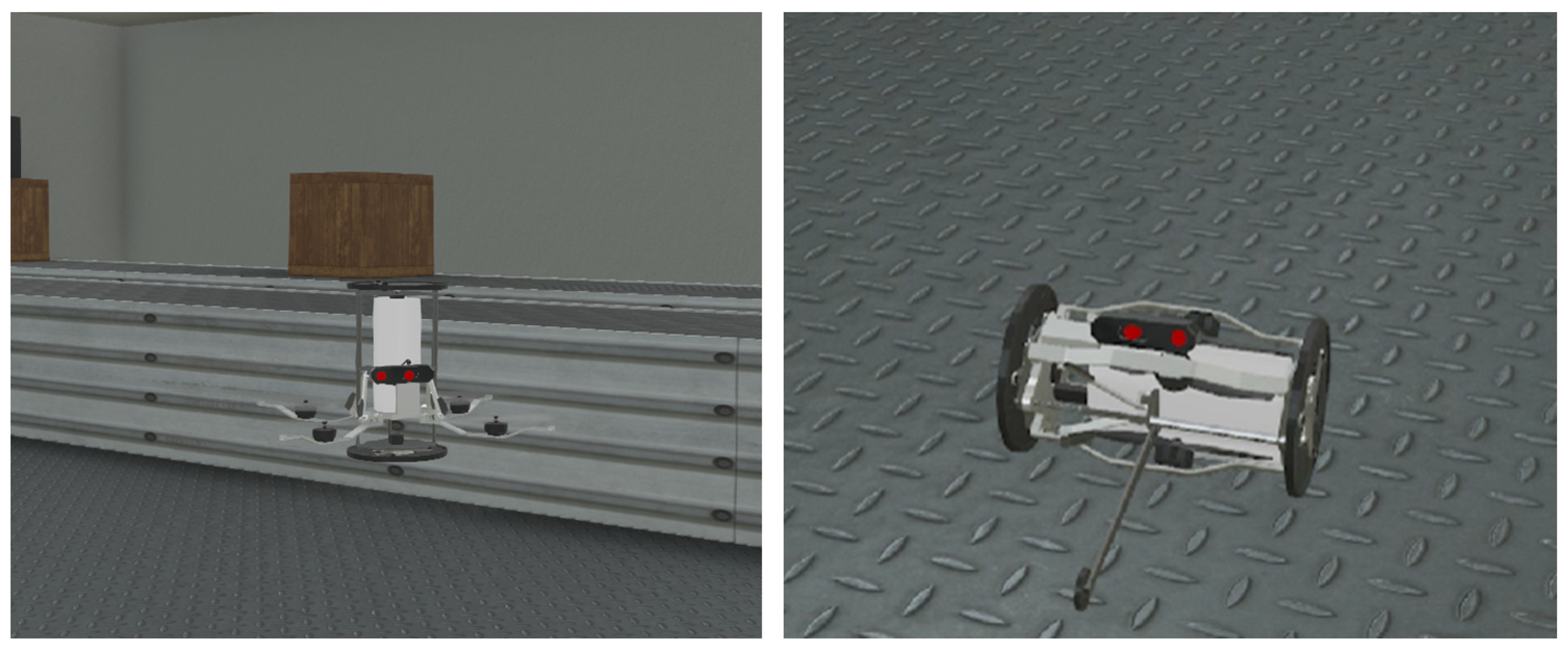
2.1. Mechanical Design
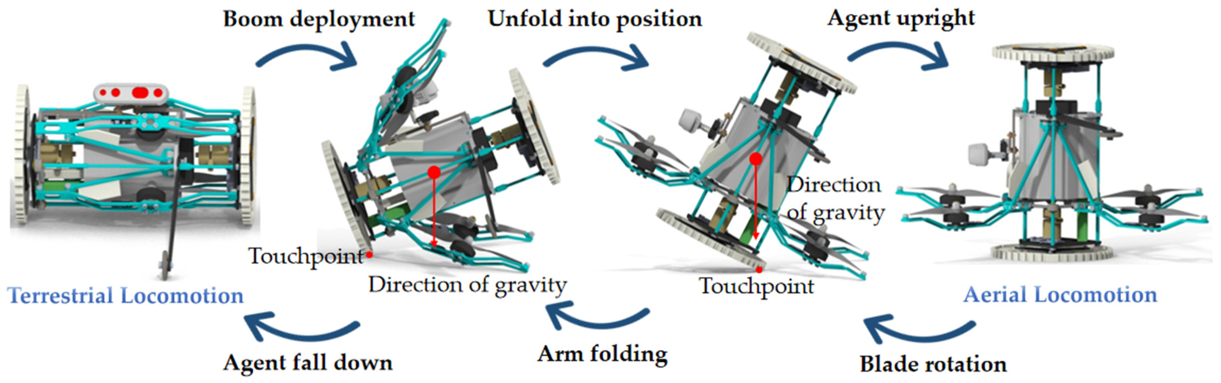
2.2. Mode Switching
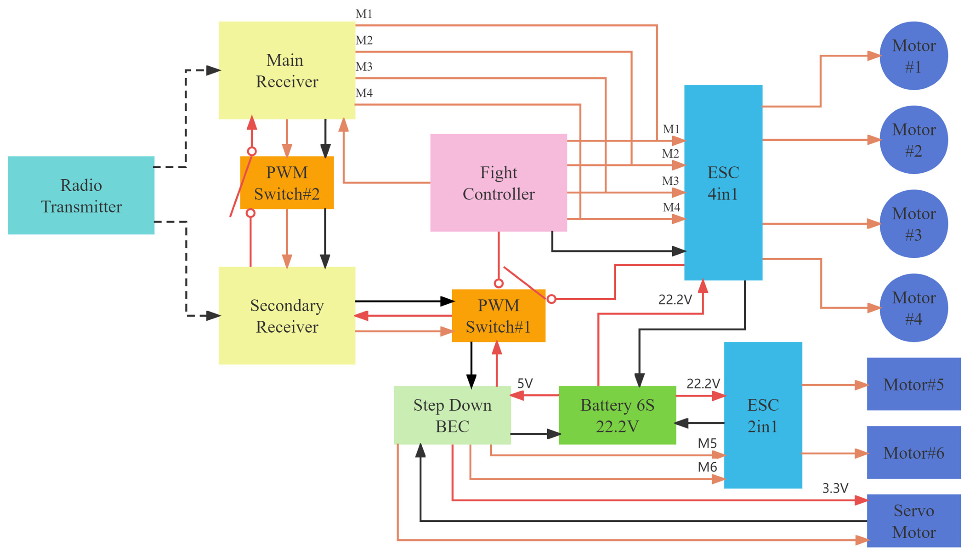
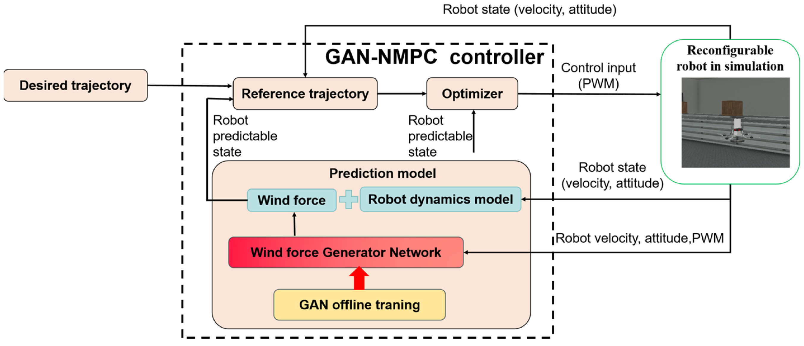
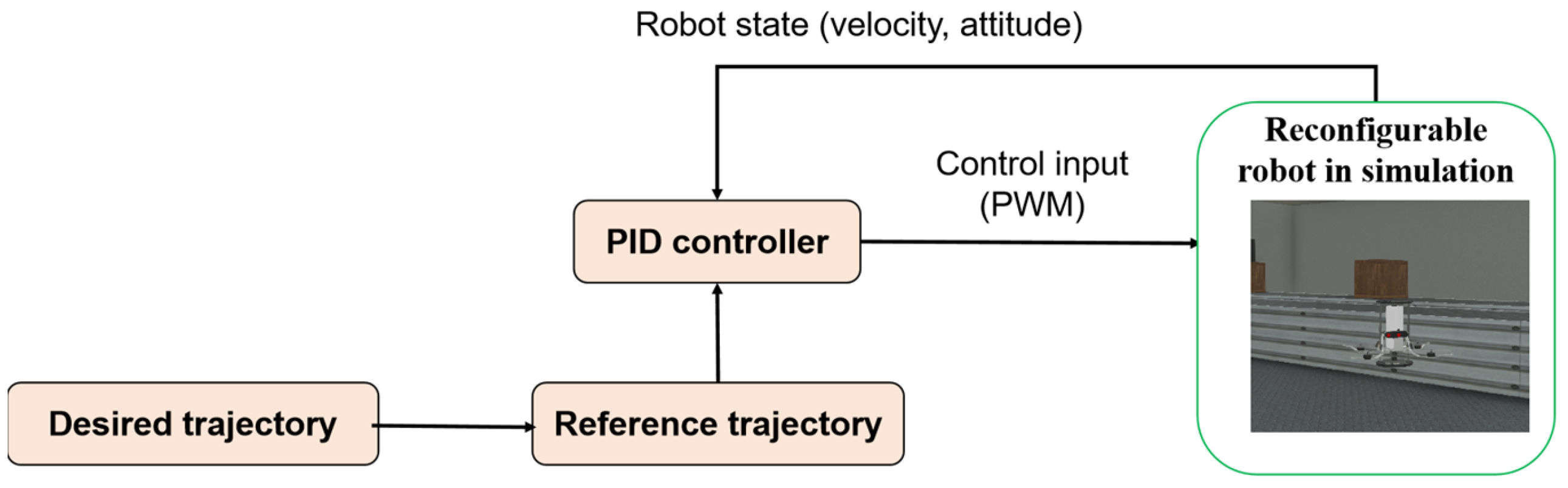
2.3. Control Scheme
3. Robot Modeling
3.1. Robot Kinematics
- 1.
- Body Coordinate System
- 2.
- World Coordinate System
- —position of the origin of measured in
- —angles of roll (ϕ), pitch () and yaw () that parametrize locally the orientation of with respect to ;
- —linear velocity of the origin of relative to expressed in (i.e., agent-fixed linear velocity);
- —angular velocity of relative to expressed in (i.e., agent-fixed angular velocity);
- —distance from the origin of to the robot’s center of mass.
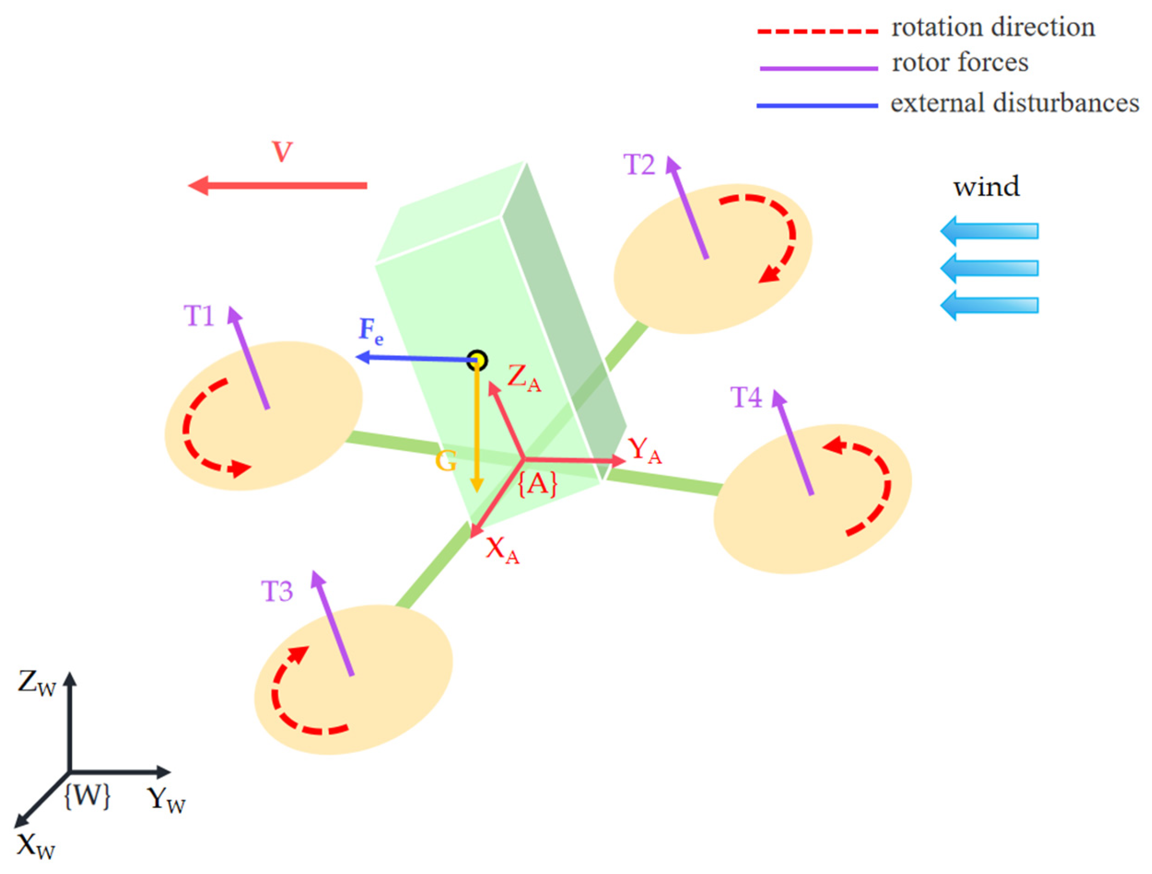
3.2. Robot Dynamics
- The center of gravity of the robot coincides with the centroid, and the mass of the robot remains unchanged during the dynamic process.
- The rotational inertia of the quadcopter is assumed to be zero.
- The robot body does not deform and is structurally symmetrical during motion.
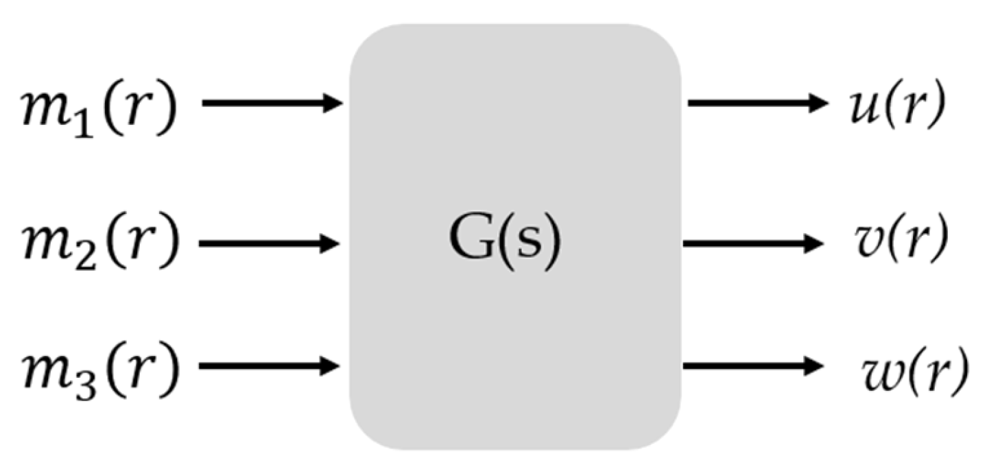
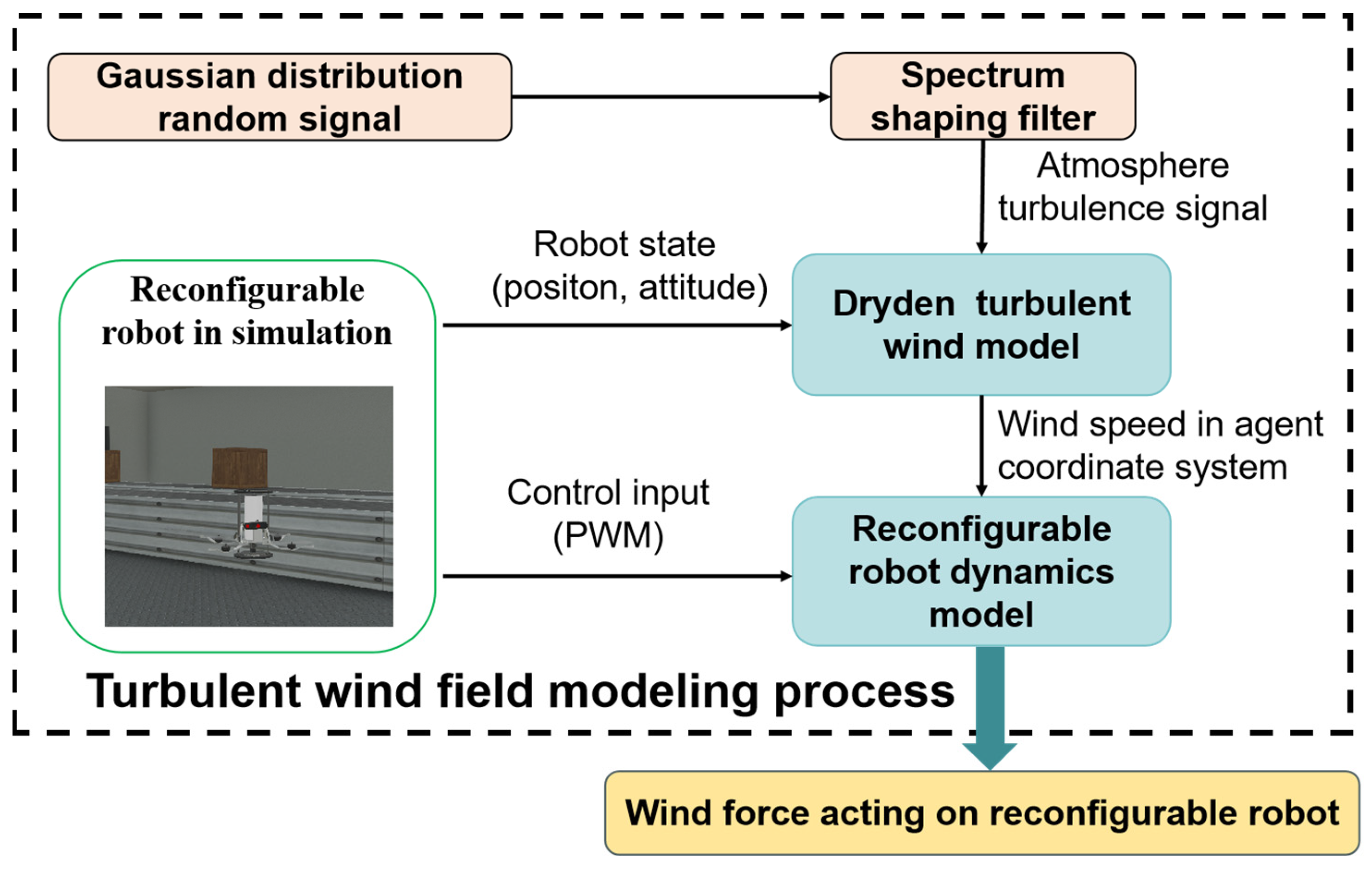
3.3. Turbulent Wind Field Modeling
4. Control Design
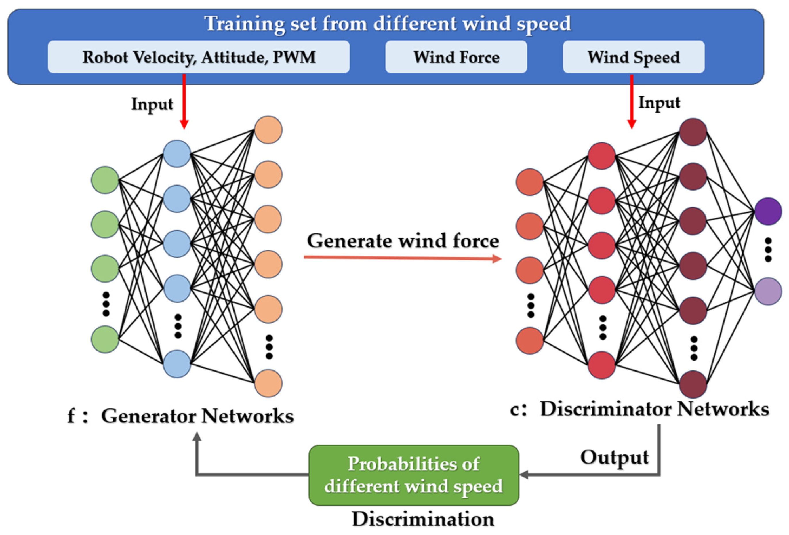
4.1. Generative Adversarial Network
4.1.1. Data Collection and Platform
4.1.2. The Principle of Generative Adversarial Networks
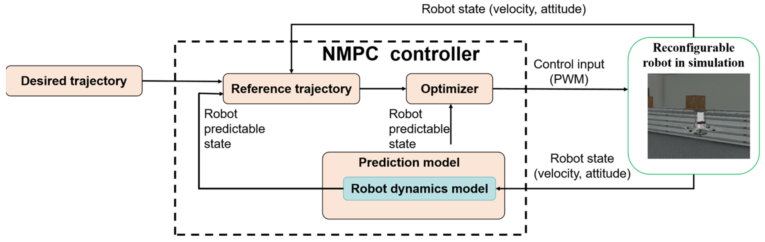
4.2. NMPC Formulation
5. Simulation and Results
5.1. Turbulent Wind Field Environment Construction
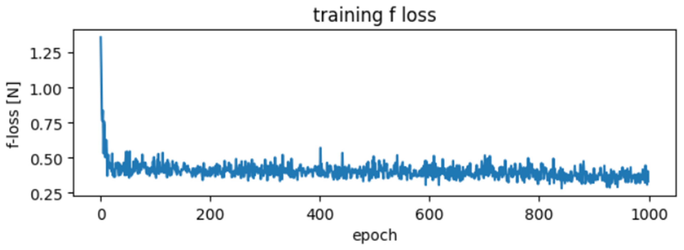
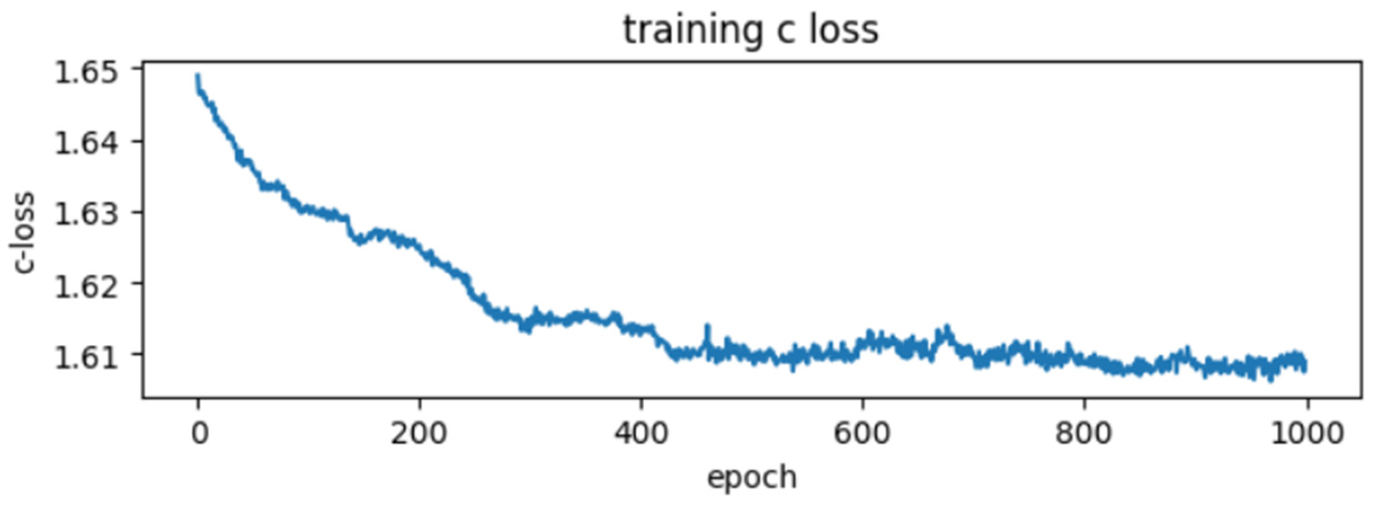
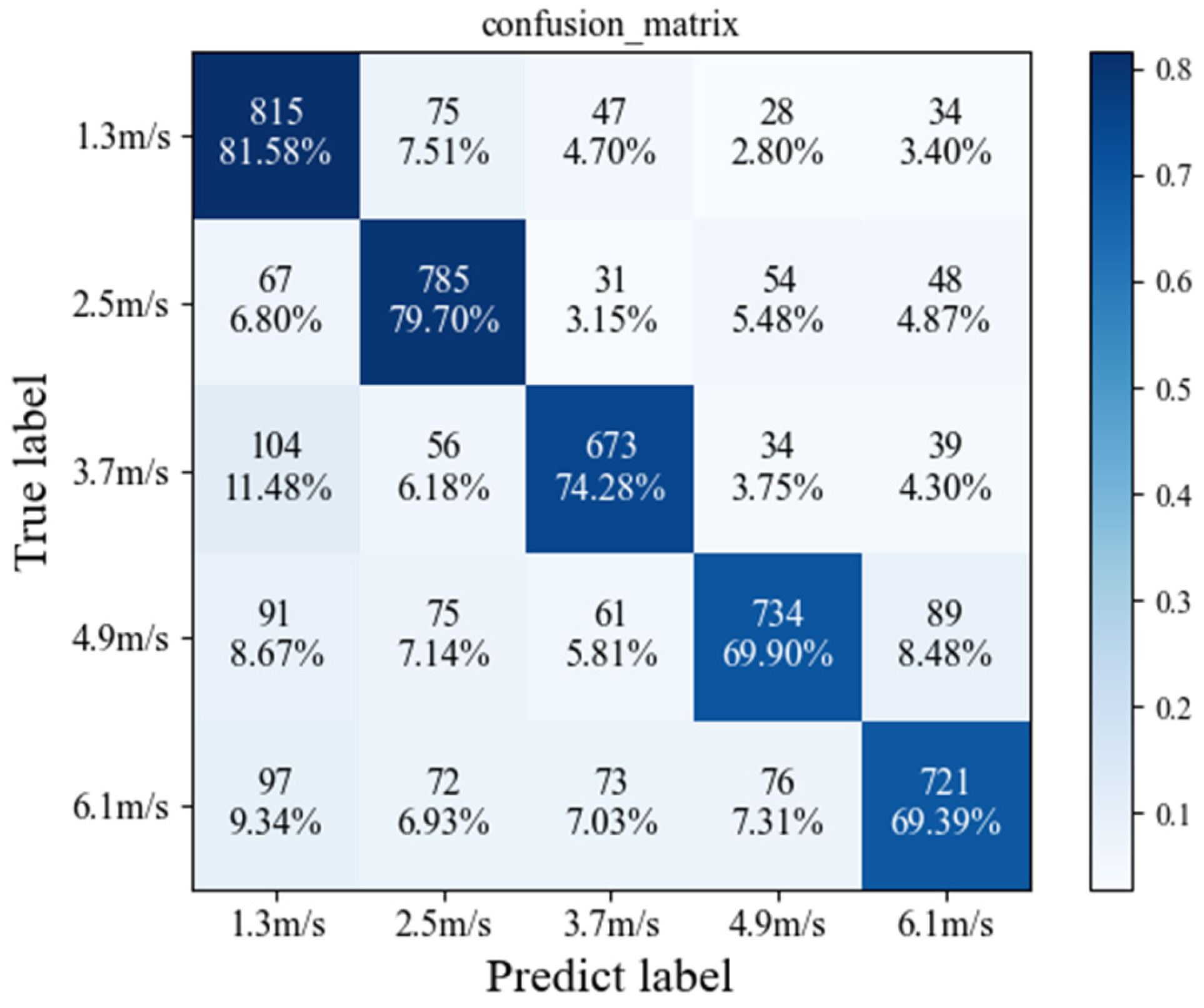
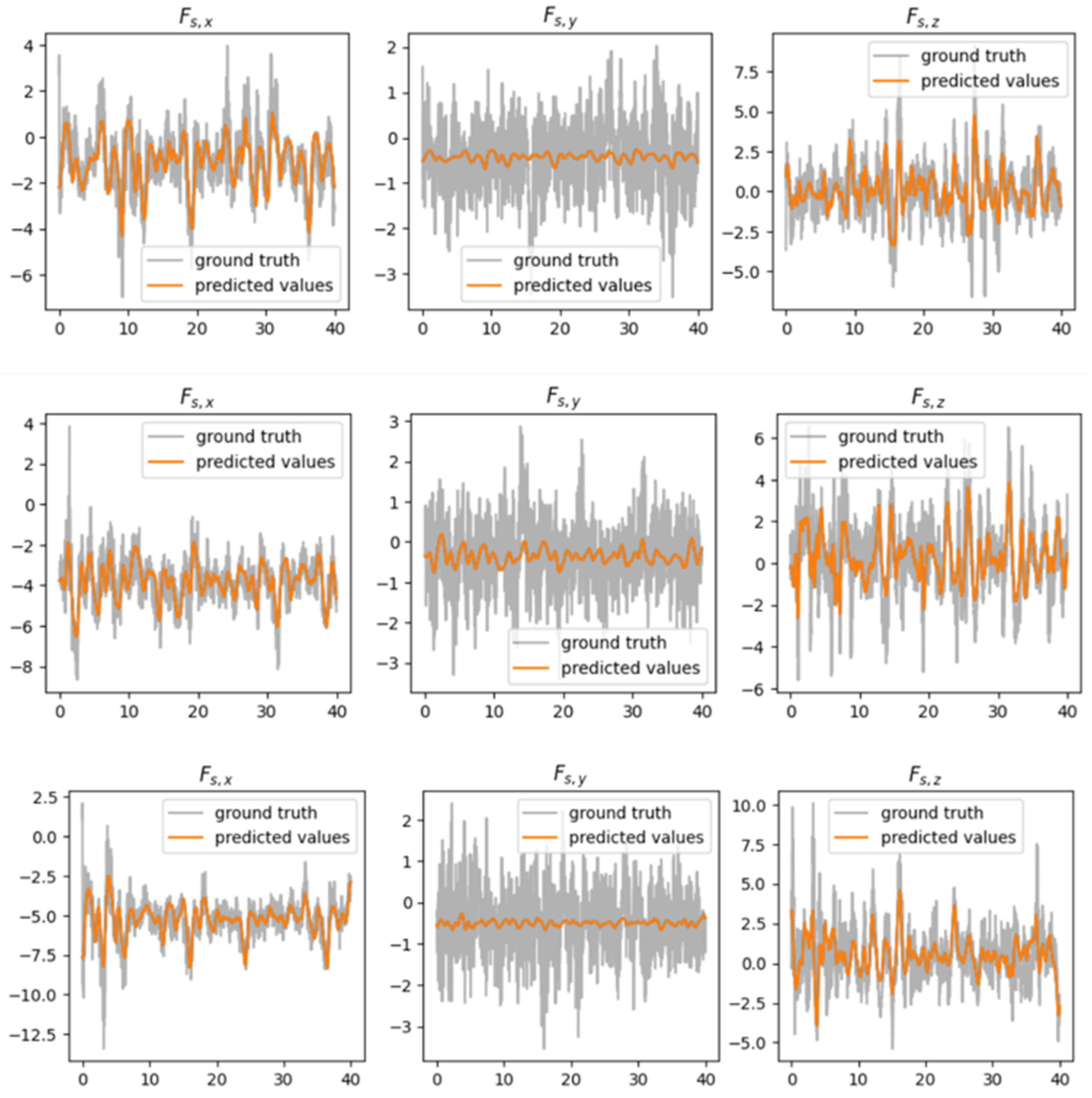
5.2. GAN Training Experiment
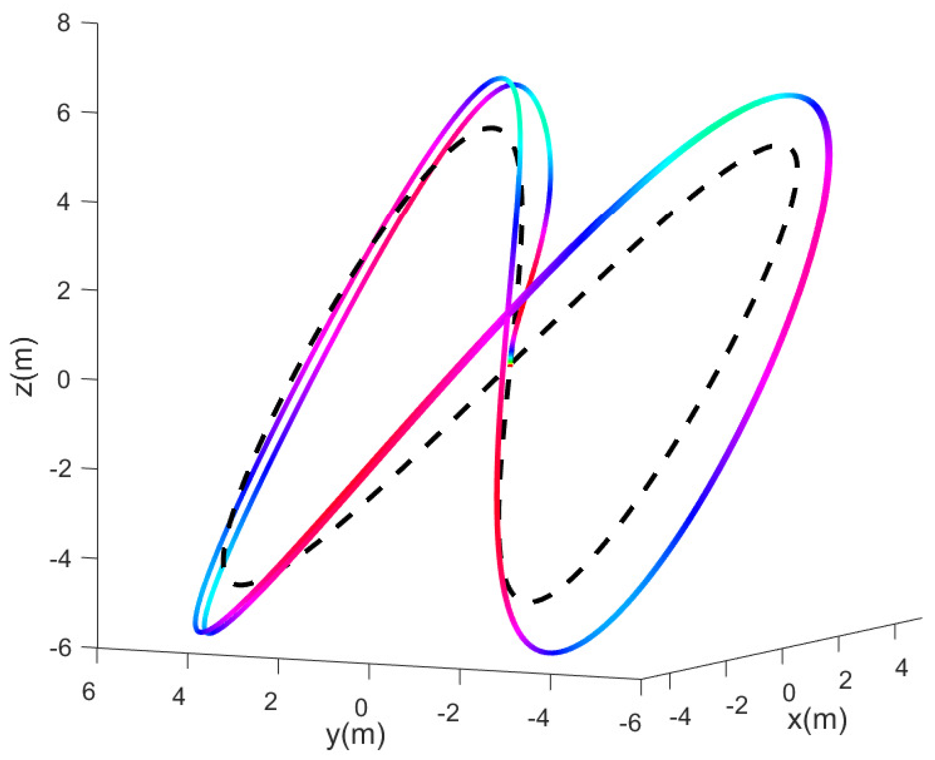
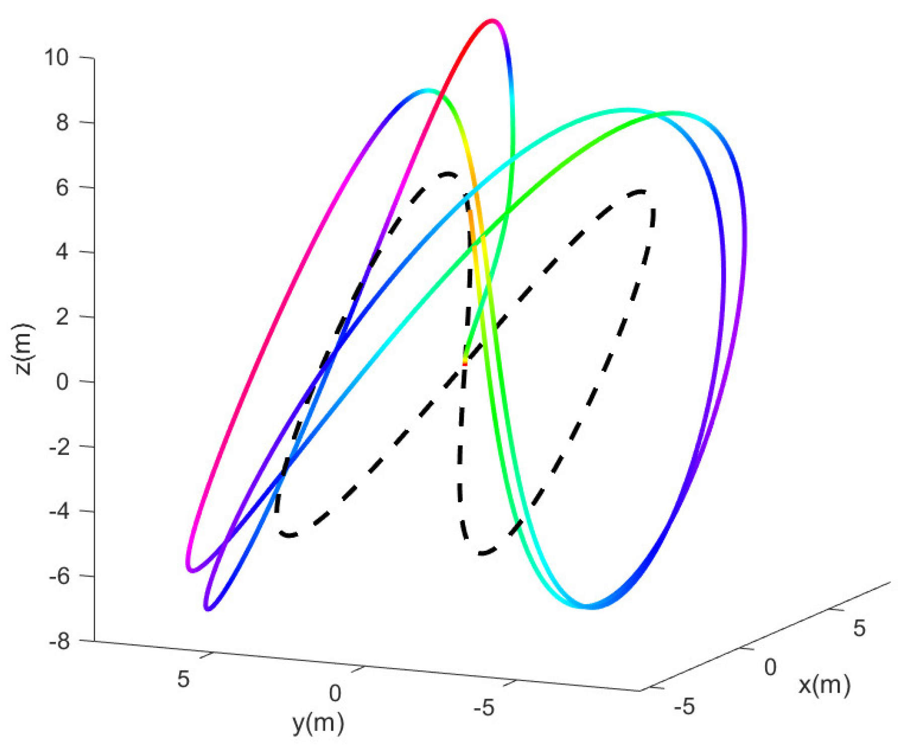
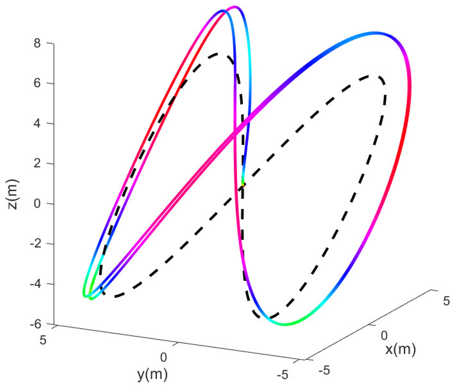
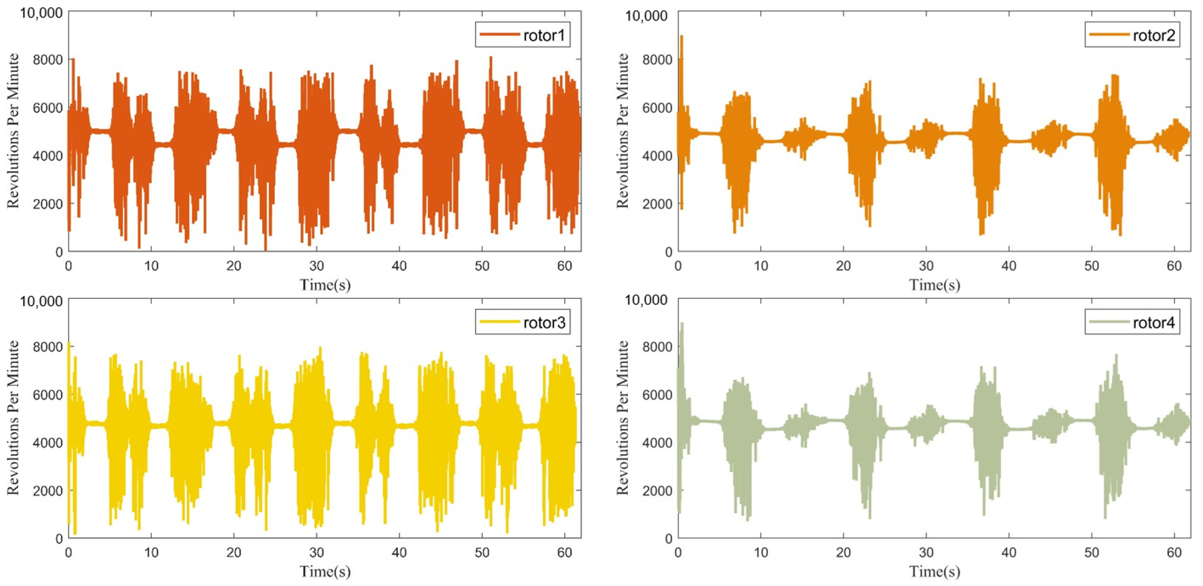
5.3. Simulation Experiment
6. Conclusions
Author Contributions
Funding
Data Availability Statement
Conflicts of Interest
References
- Fu, J.; Rota, A.; Li, S.; Zhao, J.; Liu, Q.; Iovene, E.; Ferrigno, G.; De Momi, E. Recent Advancements in Augmented Reality for Robotic Applications: A Survey. Actuators 2023, 12, 323. [Google Scholar] [CrossRef]
- Dinelli, C.; Racette, J.; Escarcega, M.; Lotero, S.; Gordon, J.; Montoyaet, J.; Dunaway, C.; Androulakis, V.; Khaniani, H.; Shao, S.; et al. Configurations and applications of multi-agent hybrid drone/unmanned ground vehicle for underground environments: A review. Drones 2023, 7, 136. [Google Scholar] [CrossRef]
- Savonitto, G.; Paganini, P.; Pavan, A.; Busetti, M.; Giustiniani, M.; Dal Cin, M.; Comici, C.; Küchler, S.; Gerin, R. Aerial Drone Imaging in Alongshore Marine Ecosystems: Small-Scale Detection of a Coastal Spring System in the North-Eastern Adriatic Sea. Remote Sens. 2023, 15, 4864. [Google Scholar] [CrossRef]
- Thomasberger, A.; Nielsen, M.M. UAV-Based Subsurface Data Collection Using a Low-Tech Ground-Truthing Payload System Enhances Shallow-Water Monitoring. Drones 2023, 7, 647. [Google Scholar] [CrossRef]
- Liu, H.; Ge, J.; Wang, Y.; Li, J.; Ding, K.; Zhang, Z.; Guo, Z.; Li, W.; Lan, J. Multi-UAV Optimal Mission Assignment and Path Planning for Disaster Rescue Using Adaptive Genetic Algorithm and Improved Artificial Bee Colony Method. Actuators 2022, 11, 4. [Google Scholar] [CrossRef]
- Choutri, K.; Lagha, M.; Meshoul, S.; Batouche, M.; Bouzidi, F.; Charef, W. Fire Detection and Geo-Localization Using UAV’s Aerial Images and Yolo-Based Models. Appl. Sci. 2023, 13, 11548. [Google Scholar] [CrossRef]
- Huang, Z.; Chen, G.; Shen, Y.; Wang, R.; Liu, C.; Zhang, L. An Obstacle-Avoidance Motion Planning Method for Redundant Space Robot via Reinforcement Learning. Actuators 2023, 12, 69. [Google Scholar] [CrossRef]
- Naghdi, M.; Hassanalian, M. Computational Analysis of Dandelion Seeds: A Novel Flight Mechanism for Design of Efficient Bioinspired Micro Drones. In Proceedings of the AIAA SCITECH 2022 Forum, San Diego, CA, USA, 3–7 January 2022. [Google Scholar]
- Tu, G.-T.; Juang, J.-G. UAV Path Planning and Obstacle Avoidance Based on Reinforcement Learning in 3D Environments. Actuators 2023, 12, 57. [Google Scholar] [CrossRef]
- Pan, N.; Jiang, J.; Zhang, R.; Xu, C.; Gao, F. Skywalker: A Compact and Agile Air-Ground Omnidirectional Vehicle. IEEE Robot. Autom. Lett. 2023, 8, 2534–2541. [Google Scholar] [CrossRef]
- Liu, Z.; Song, M.; Liu, Y.; Bai, B. Design, Modeling and Simulation of a Reconfigurable Land-Air Amphibious Robot. In Proceedings of the 2021 IEEE 11th Annual International Conference on CYBER Technology in Automation, Control, and Intelligent Systems (CYBER), Jiaxing, China, 27–31 July 2021. [Google Scholar]
- Khalil, A.; Jaradat, M.A.; Mukhopadhyay, S.; Abdel-Hafez, M.F. Autonomous Control of a Hybrid Rolling and Flying Caged Drone for Leak Detection in HVAC Ducts. IEEE/ASME Trans. Mechatron. 2023, 1, 1–13. [Google Scholar] [CrossRef]
- Choi, H.C.; Wee, I.; Corah, M.; Sabet, S.; Kim, T.; Touma, T.; Agha-mohammadi, A.A. Baxter: Bi-modal aerial-terrestrial hybrid vehicle for long-endurance versatile mobility. In Experimental Robotics: The 17th International Symposium; Springer International Publishing: Berlin/Heidelberg, Germany, 2021; Volume 19, pp. 60–72. [Google Scholar]
- Premachandra, C.; Otsuka, M.; Gohara, R.; Ninomiya, T.; Kato, K. A study on development of a hybrid aerial/terrestrial robot system for avoiding ground obstacles by flight. IEEE/CAA J. Autom. Sin. 2018, 6, 327–336. [Google Scholar] [CrossRef]
- Kim, K.; Spieler, P.; Lupu, E.S.; Ramezani, A.; Chung, S.J. A bipedal walking robot that can fly, slackline, and skateboard. Sci. Robot. 2021, 6, 59. [Google Scholar] [CrossRef] [PubMed]
- Jia, H.; Bai, S.; Ding, R.; Shu, J.; Deng, Y.; Khoo, B.L.; Chirarattananon, P. A quadrotor with a passively reconfigurable airframe for hybrid terrestrial locomotion. IEEE/ASME Trans. Mechatron. 2022, 27, 4741–4751. [Google Scholar] [CrossRef]
- David, N.B.; Zarrouk, D. Design and analysis of FCSTAR, a hybrid flying and climbing sprawl tuned robot. IEEE Robot. Autom. Lett. 2021, 6, 6188–6195. [Google Scholar] [CrossRef]
- Beck, A.T. Optimal design of redundant structural systems: Fundamentals. Eng. Struct. 2020, 219, 110542. [Google Scholar] [CrossRef]
- He, Y.; Wang, W.; Wang, Q.; Wang, Y. Novel Design of the Wheel-footed obstacle-surmounting Robot. J. Phys. Conf. Ser. 2020, 1550, 022019. [Google Scholar] [CrossRef]
- Tajima, Y.; Hiraguri, T.; Matsuda, T.; Imai, T.; Hirokawa, J.; Shimizu, H.; Kimura, T.; Maruta, K. Analysis of Wind Effect on Drone Relay Communications. Drones 2023, 7, 182. [Google Scholar] [CrossRef]
- Sorbelli, F.B.; Corò, F.; Das, S.K.; Pinotti, C.M. Energy-constrained delivery of goods with drones under varying wind conditions. IEEE Trans. Intell. Transp. Syst. 2020, 22, 6048–6060. [Google Scholar] [CrossRef]
- Wen, S.; Han, J.; Ning, Z.; Lan, Y.; Yin, X.; Zhang, J.; Ge, Y. Numerical analysis and validation of spray distributions disturbed by quad-rotor drone wake at different flight speeds. Comput. Electron. Agric. 2019, 166, 105036. [Google Scholar] [CrossRef]
- Santoso, F.; Garratt, M.A.; Anavatti, S.G. Hybrid PD-fuzzy and PD controllers for trajectory tracking of a quadrotor unmanned aerial vehicle: Autopilot designs and real-time flight tests. IEEE Trans. Syst. Man Cybern. Syst. 2019, 51, 1817–1829. [Google Scholar] [CrossRef]
- Okyere, E.; Bousbaine, A.; Poyi, G.T.; Joseph, A.K.; Andrade, J.M. LQR controller design for quad-rotor helicopters. J. Eng. 2019, 17, 4003–4007. [Google Scholar] [CrossRef]
- Islam, M.; Okasha, M.; Sulaeman, E. A model predictive control (MPC) approach on unit quaternion orientation based quadrotor for trajectory tracking. Int. J. Control Autom. Syst. 2019, 17, 2819–2832. [Google Scholar] [CrossRef]
- Creswell, A.; White, T.; Dumoulin, V.; Arulkumaran, K.; Sengupta, B.; Bharath, A.A. Generative adversarial networks: An overview. IEEE Signal Process. Mag. 2018, 35, 53–65. [Google Scholar] [CrossRef]
- Karras, T.; Aittala, M.; Hellsten, J.; Laine, S.; Lehtinen, J.; Aila, T. Training generative adversarial networks with limited data. Adv. Neural Inf. Process. Syst. 2020, 33, 12104–12114. [Google Scholar]
- O’Connell, M.; Shi, G.; Shi, X.; Azizzadenesheli, K.; Anandkumar, A.; Yue, Y.; Chung, S.J. Neural-fly enables rapid learning for agile flight in strong winds. Sci. Robot. 2022, 7, 66. [Google Scholar] [CrossRef]
- Li, J.; Li, Y. Dynamic analysis and PID control for a quadrotor. In Proceedings of the 2011 IEEE International Conference on Mechatronics and Automation, Beijing, China, 7–10 August 2011; pp. 573–578. [Google Scholar]
- Zavala, V.M.; Biegler, L.T. The advanced-step NMPC controller: Optimality, stability, and robustness. Automatica 2009, 45, 86–93. [Google Scholar] [CrossRef]


| Mode Descriptions | Rotor Protection | |
|---|---|---|
| Baxter | Two modes of operation, aerial and terrestrial. Employs two novel hardware mechanisms: the M-Suspension and the Decoupled Transmission | Spherical Cage Protection |
| Hybrid aerial/terrestrial robot | A quadcopter with a mechanism for ground movement. Not use power dedicated to ground movement, and instead uses the flight mechanism of the quadcopter to achieve ground movement as well. | Rotor exposed outside None close mechanism |
| LEONARDO | Flying and walking. Using synchronized control of distributed electric thruster and a pair of multi-jointed legs, the two modes of flight and walking are interchanged. | Rotor exposed outside None close mechanism |
| Hybrid Terrestrial Ouadrotor | Flying and rolling. The transitions between flight and rolling are accomplished with a highly dynamic maneuver, the robot remains compact and lightweight. | Rotor exposed outside None close mechanism |
| FCSTAR | Climbing walls and flying. By using thrust reversal and its 4-wheel drive, the robot can drive over steep slopes. | Rotor exposed outside None close mechanism |
| Component | Parameters |
|---|---|
| Mass (with battery) | 1.86 kg |
| Folded size | 284 × 168 × 168 mm3 |
| Unfolded size | 410 × 410 × 284 mm3 |
| Propeller size (maximum boundary) | 170 mm × 20 mm |
| Minimum pass size | 390 mm × 200 mm |
| Battery of robot | 6 S, 22.2 V, 2700 mAh |
| Path planning and decision response time | ≤200 ms |
| Maximum flight time | ≥15 min |
| Mode switching time | ≤5 s |
| Rolling speed | 1.86 m/s |
| Creep speed | 0.87 m/s |
| Flight speed | 10.66 m/s |
| Parameters | Value |
|---|---|
| Number of adaptive sampling points: K | 32 |
| Number of sampling points for network training: B | 256 |
| Adversarial loss coefficient: α | 0.01 |
| Network learning rate | 5 × 10⁻⁴ |
| Network update probability: h | 0.5 |
| The maximum binomial γ of a | 10 |
| Epochs | 1000 |
| Situation | Before Learning (N) | After Learning Error (N) |
|---|---|---|
| 1.3 m/s | 1.20 | 0.54 |
| 2.5 m/s | 2.17 | 0.85 |
| 3.7 m/s | 3.58 | 0.89 |
| 4.9 m/s | 6.69 | 1.00 |
| 6.1 m/s | 11.41 | 1.08 |
| Model | PID | NMPC | GAN-NMPC | ||||
|---|---|---|---|---|---|---|---|
| Wind | RMS | MEAN | RMS | MEAN | RMS | MEAN | |
| 12.1 m/s | 63.7 | 59.4 | 31.4 | 28.7 | 13.9 | 11.2 | |
| 8.5 m/s | 31.6 | 27.2 | 16.3 | 13.9 | 7.3 | 6.3 | |
| 4.2 m/s | 16.2 | 14.6 | 10.7 | 9.9 | 3.7 | 2.9 | |
Disclaimer/Publisher’s Note: The statements, opinions and data contained in all publications are solely those of the individual author(s) and contributor(s) and not of MDPI and/or the editor(s). MDPI and/or the editor(s) disclaim responsibility for any injury to people or property resulting from any ideas, methods, instructions or products referred to in the content. |
© 2024 by the authors. Licensee MDPI, Basel, Switzerland. This article is an open access article distributed under the terms and conditions of the Creative Commons Attribution (CC BY) license (https://creativecommons.org/licenses/by/4.0/).
Share and Cite
Chang, Q.; Yu, B.; Ji, H.; Li, H.; Yuan, T.; Zhao, X.; Ren, H.; Zhan, J. Design and Control of a Reconfigurable Robot with Rolling and Flying Locomotion. Actuators 2024, 13, 27. https://doi.org/10.3390/act13010027
Chang Q, Yu B, Ji H, Li H, Yuan T, Zhao X, Ren H, Zhan J. Design and Control of a Reconfigurable Robot with Rolling and Flying Locomotion. Actuators. 2024; 13(1):27. https://doi.org/10.3390/act13010027
Chicago/Turabian StyleChang, Qing, Biao Yu, Hongwei Ji, Haifeng Li, Tiantian Yuan, Xiangyun Zhao, Hongsheng Ren, and Jinhao Zhan. 2024. "Design and Control of a Reconfigurable Robot with Rolling and Flying Locomotion" Actuators 13, no. 1: 27. https://doi.org/10.3390/act13010027
APA StyleChang, Q., Yu, B., Ji, H., Li, H., Yuan, T., Zhao, X., Ren, H., & Zhan, J. (2024). Design and Control of a Reconfigurable Robot with Rolling and Flying Locomotion. Actuators, 13(1), 27. https://doi.org/10.3390/act13010027