Experimental Research on Avoidance Obstacle Control for Mobile Robots Using Q-Learning (QL) and Deep Q-Learning (DQL) Algorithms in Dynamic Environments

Abstract

This study provides simulation and experimental results on techniques for avoiding static and dynamic obstacles using a deep Q-learning (DQL) reinforcement learning algorithm for a two-wheel mobile robot with independent control. This method integrates the Q-learning (QL) algorithm with a neural network, where the neural networks in the DQL algorithm act as approximators for the Q matrix table for each pair (state–action). The effectiveness of the proposed solution was confirmed through simulations, programming, and practical experimentation. A comparison was drawn between the DQL algorithm and the QL algorithm. Initially, the mobile robot was connected to the control script using the Robot Operating System (ROS). The mobile robot was programmed in Python within the ROS operating system, and the DQL controller was programmed in Gazebo software. The mobile robot underwent testing in a workshop with various experimental scenarios considered. The DQL controller displayed improvements in computation time, convergence time, trajectory planning accuracy, and obstacle avoidance. As a result, the DQL controller surpassed the QL algorithm in terms of performance.

1. Introduction

Mobile robots play a crucial role in societal advancement, undertaking perilous or challenging tasks for humans, such as search and rescue operations, and aiding in epidemic-stricken areas and the exploration of remote planets. Consequently, designing such robots necessitates meticulous trajectory planning—a pivotal aspect [1]. This planning emphasizes creating the shortest distance, minimizing time, conserving energy, and circumventing obstacles enroute to the target [2]. Mobile robot trajectory planning encompasses global path planning, local path planning, static path planning, and dynamic path planning [3,4].

Recent research has seen an increase in trajectory-planning studies for mobile robots to evade obstacles in their operational surroundings. These studies involve linear, nonlinear, and intelligent algorithms. In one study [5], mobile robots utilized an artificial potential field (APF) algorithm for path planning. Another study explored the checkerboard method, with the researchers frequently employing a simulation algorithm to determine the optimal trajectory for mobile robots [6]. Additionally, various pathfinding algorithms for static obstacle avoidance have been utilized, such as the A* algorithm [7], the D algorithm [8], the DWA algorithm [9], the random tree algorithm (RRT) [10], the genetic algorithm (GA) [11], particle swarm optimization (PSO) [12], ant colony optimization [13], the gravity search algorithm (GSA) [14], and pigeon-inspired optimization [15]. A robot is moved according to the trajectories set based on the PID-FLC controller [16], and intelligent control for mobile robots based on a fuzzy logic controller [17] has gained popularity. Upon analyzing the aforementioned research findings, it is evident that mobile robots can swiftly and accurately operate in static environments (where comprehensive knowledge of the area exists) by adjusting their movement speed and trajectory to avoid obstacles. However, orbital navigation planning for mobile robots proves effective in dynamic environments (characterized by complexity and numerous variables) [18]. Consequently, AI algorithms are recommended for planning mobile robot trajectories in dynamic environments, such as the GA-fuzzy method [19], ANFIS [20], reinforcement learning (RL), and machine learning (ML). These AI algorithms allow mobile robot trajectories to be trained and updated online in real time [21].

Building on a previous investigation [22], researchers have extensively utilized the RL algorithm in gaming and IT. However, many scholars have also applied this algorithm’s advantageous features, such as simple controller design and orbital navigation planning, to mobile robots [23,24]. Despite this, the RL algorithm only marginally improves pathing and increases computation time for convergence. With reference to studies [25,26,27], the Q-learning (QL) algorithm charts the mobile robot’s trajectory by learning from past environmental observations. The QL algorithm has improved computation speed and convergence. However, it computes the Q values of states to expand the action values of the neural network. Since accessing all action–state pairs in complex, dynamic environments are necessary, planning the mobile robot’s trajectory takes a substantial amount of time.

Consequently, several studies have proposed various solutions to mitigate the drawbacks of traditional QL algorithms. Nakashima and Ishibashi [28] utilized a fuzzy set to moderate the appropriate Q-value initialization, hastening convergence. In a separate study, Jiang and Xin [29] introduced a QL algorithm that generates undefined state variables using a new technique for continuous space division and learning planning in an unknowable dynamic environment.

Additionally, researchers have recommended an integrated learning strategy based on spatial allocation to expedite the learning process. When combined with the QL method, the state–action–reward–state–action (SARSA) technique enabled Wang et al. [30] to achieve rapid convergence, with the study results indicating reduced learning time. Das et al. [31] devised an alternative to QL to address the convergence rate issue. To update the Q table in a more organized manner with reduced time and space complexity, Goswami et al. [32,33] enhanced the basic QL algorithm. The Q values are preserved in the Q table at the best action values for each state, resulting in significant time savings. The researchers established a distinct field for the operation of each table. Numerous QL algorithms have lessened the computation and convergence times for planning mobile robot trajectories in intricate and dynamic environments. However, to enhance navigation control in both static and dynamic environments for mobile robots, this study developed a deep Q-learning (DQL) algorithm. DQL contains neural networks that are Q-value estimators for each pair (state-action).

This paper makes several key contributions:

-

Successful studies on the navigation controller of mobile robot paths based on the DQL algorithm based on the ROS operating system through simulation and experimental results.

-

Simulation and experimental results for mobile robots using the DQL algorithm compared to the QL algorithm have demonstrated the efficiency and superiority of the proposed algorithm in terms of (1) the proposed DQL algorithm being able to quickly and safely generate optimal and near-optimal paths; (2) the mobile robot moving quickly to the required location and avoiding obstacles; (3) the DQL algorithm not needing a defined environment and lacking a good trade-off between convergence speed and path length and the algorithm requiring a few milliseconds to compute a good solution in terms of length and safety; (4) the proposed DQL performance being improved compared with the performance of the latest related work; and (5) the suggested DQL increasing the route quality with regard to the length, computation time, and robot safety.

The remainder of this paper is organized as follows. The path planning control problems for mobile robots are described in Section 1. The mathematical modeling of the operating system for a mobile robot is described in Section 2. The design of the optimal path for mobile robots using the DQL algorithm is described in Section 3. Finally, the solution’s effectiveness is tested, compared, and analyzed through simulations and experiments with the QL algorithm in Section 4.

2. Mathematical Modeling of an Operating System for a Mobile Robot

2.1. Obstacle Modeling in the Mobile Robot Operating Environment

The obstacle model was built on a rectangular box. Among the static and dynamic path optimization techniques that collect obstacle estimates, the optimal geometry allows for the easy estimation of any obstacle shape. The obstacles formed using cubes are shown in Figure 1. In Figure 1a, by using this geometry to plan the robot in 2D, blocks can be replaced while avoiding 3D obstacles. A realistic scene with 3D blocks (chairs, tables, etc.) is shown in Figure 1b. A binary map of the modeled environment is shown in Figure 1c.

2.2. Mathematical Model

The mobile robot moves from the start point ($x_s,y_s$) to the destination point target ($x_T,y_T$); the purpose of robot path planning is to find the optimal path from the start point to the target point. This path is connected by n nodes ($N_i,i=1\dots n$), and (n − 1) each segment is two consecutive nodes connected to each other. We assume that the robot moves in an environment with m known obstacles, as shown in Figure 1. Each obstacle is modeled surrounded by a rectangle with four vertices $p_1(x_1,y_1)\mathrm{}\dots p_4(x_4,y_4)$ and four edges $obs\_se{g}_{tj}(t\in \left\{1\dots 4\right\},j\in \left\{1\dots m\left\{\right\}\right\}$, where $p_1$ is the bottom left corner of the rectangle. Similar to obstacles in the environment, the mobile robot is also estimated by a rectangle of four points, and their coordinates change according to the robot’s current position. The mathematical equation of each segment defined by the two points ($p_k,p_l$) of a rectangle enclosing an obstacle is given by Equation (1):

$$seg\left(p_k,p_l\right)=\{\begin{array}{c}y-y_k=\frac{y_l-y_k}{x_l-x_k}\left(x-x_k\right)\\ Min\left(x_l,x_k\right)\le x\le Max\left(x_l,x_k\right)\end{array}$$

(1)

The following notation describes the indices and parameters used in the mathematical model:

N: number of nodes on the trajectory created from the starting point to the destination.

m: number of obstacles in the environment.

• $i(i\in \left\{1\dots n\left\{\right\}\right\}$: fragment index generated by the node $i$ and $i+1$.
• $j\left(j\in \left\{1\dots m\right\}\right)$: index of the $j^{th}$ obstacle in the navigation environment.
• $k,l\left(k,l\in \left\{1\dots 4\right\}\right)$: indices of the point that defines an obstacle.
• $r\left(r\in \left\{1\dots 4\right\}\right)$: index of segment r from the rectangle approximating the mobile robot.
• $t\left(t\in \left\{1\dots 4\right\}\right)$: index of the segment r that defines the rectangle of an obstacle.
• $N_i:i^{th}$ node of the path.
• $ob{s}_j\left(j\in \left\{1\dots m\right\}\right):j^{th}$ obstacle.
• $path\_se{g}_i\left(N_i,N_{i+1}\right)\left(i\in \left\{1\dots n-1\right\}\right):i^{th}$ segment of the path defined by two nodes $\left(N_i,N_{i+1}\right)$.
• $obs\_se{g}_{lj}\left(p_k,p_l\right)\left(k,l\in \left\{1\dots 4\right\}\right)j\left(j\in \left\{1\dots m\right\}\right):l^{th}$ segment of the $j^{th}$ obstacle defined by two points ($p_k,p_l$).
• CurrentPos: current location of the robot.
• $Rob\_se{g}_r\left(p_k,p_l\right)\left(r,k,l\in \left\{1\dots 4\right\}\right):r^{th}$ segment of the rectangle approximating the robot.

The mathematical model’s decision variables are computed as follows:

$$B_{i,t,j}=\{\begin{array}{c}\begin{array}{c}1if\exists P_1,P_2|\left\{P_1,P_1\right\}\in \left(path\_se{g}_i\right)\wedge \left\{P_1,P_1\right\}\in \left(obs\_se{g}_{tj}\right)\hfill \\ \forall j(j\in \left\{1\dots m\right\},\forall t\left(t\in \left\{1\dots 4\right\}\right),\forall i(i\in \left\{1\dots n\left\{\right\}\right\}\end{array}\\ 0\begin{array}{ccc}& & \end{array}\begin{array}{ccc}& & \begin{array}{cccc}& & & Otherwise\end{array}\end{array}\hfill \end{array}$$

(2)

$$A_{i,t,j}=\{\begin{array}{c}\begin{array}{c}1if\exists P_1,P_2|\left\{P_1,P_1\right\}\in \left(path\_se{g}_r\right)\wedge \left\{P_1,P_1\right\}\in \left(obs\_se{g}_{tj}\right)\hfill \\ \forall j(j\in \left\{1\dots m\right\},\forall r,t\left(t\in \left\{1\dots 4\right\}\right),\end{array}\\ 0\begin{array}{cccc}& & & \begin{array}{cccc}& & & Otherwise\end{array}\end{array}\hfill \end{array}$$

(3)

The objective function is to find the shortest path according to Equation (4):

$$Minimize\left({\sum }_{1=1}^{i=n-1}\sqrt{{(x_{i+1}-x_i)}^2+{(y_{i+1}-y_i)}^2},\forall \in \left\{1\dots n-1\right\}\right)$$

(4)

Equation (5) requires each node to be unique:

$$\left(x_{i+1}\ne x_i\right)\vee (y_{i+1}\ne y_i),\forall i\in \left\{1\dots n-1\right\}$$

(5)

The path segments do not overlap in the environment with Equation (6):

$${\sum }_{i=1}^{i=n-1}{\sum }_{j=1}^{j=m}{B}_{i,t,j}=0,\forall i\in \left\{1\dots n\right\},t\in \left\{1\dots 4\right\},j\in \left\{1\dots m\left\{\right\}\right\}$$

(6)

The way for nodes of the robot to overcome obstacles is calculated by Equation (7).

$${\sum }_{j=1}^{j=m}{A}_{r,t,j}=0,\forall r,t\in \left\{1\dots 4\right\},j\in \left\{1\dots m\left\{\right\}\right\}$$

(7)

All variables A and B must be binary to satisfy the requirement of Equation (8):

$$B_{i,t,j}\in \left\{0,1\right\},A_{r,t,j}\in \left\{0,1\right\}\forall i\in \left\{1\dots n\right\},r,t\in \left\{1\dots 4\right\},j\in \left\{1\dots m\left\{\right\}\right\}$$

(8)

3. Deep Q-Learning and Q-Learning Algorithms in Path Planning for Mobile Robots

3.1. Q-Leaning

The Q-learning (QL) algorithm uses the concept of reward and punishment as created in the environment in Figure 2. Figure 2 illustrates how a mobile robot selects an action based on the appropriate policy, executes that action, and receives status (s) and rewards (r) from the navigation environment. A state contains the robot’s current position in its workspace while optimizing paths, while an action is a movement whereby the robot transitions from one state to another.

The Q value was built for the robot to decide to earn the greatest reward. This is calculated as follows in Equation (9):

$$Q\left(s_t,a_t\right)+\alpha \left[r\left(s_t,a_t\right)+\gamma \underset{aϵA}{\max }Q(\left(s_{t+1},a\right)\right]-Q(\left(s_t,a_t\right)$$

(9)

where $\alpha$ represents the learning rate, γ is the discount factor, and $s_t\underset{a\in A}{max}Q(s_{t+1},a)$ signifies the maximum Q-value among all feasible actions in the new state $a_t$, and denotes the immediate reward/penalty earned by the agent after executing a move at state $s_{t+1}$.

Based on Equation (9), it is a state matrix which acts as a lookup table. From there, for each state of the robot, we found the action with the most significant Q value (Figure 3).

Reinforcement learning is a random process; therefore, the Q values will differ before and after the action. This is called a temporary difference, based on Equation (10).

$$TD\left(a,s\right)+r\left(s_t,a_{t }\right)+\gamma \underset{aϵA}{\max }Q(\left(s_{t+1},a\right)]-Q(\left(s_t,a_{t }\right)$$

(10)

Thus, the matrix $Q(s_t,a_t)$ needs to update the weights based on Equation (11):

$$Q_t(s_t,a_t)=Q_{t-1}(s_t,a_t)+\alpha T{D}_t(a_t,s_t)$$

(11)

where α is an arithmetic coefficient. Through the times the robot performs actions, $Q(s_t,a_t)$ will gradually converge.

The programming program for the Q-learning algorithm for robot pathfinding is expressed as follows (Algorithm 1):

Algorithm 1: Classical Q-learning algorithm begins

Initialization: $\mathit{Q}\left({\mathit{s}}_{\mathit{t}},{\mathit{a}}_{\mathit{t}}\right)\leftarrow \left\{\mathbf{0}\right\}$, (states and m actions) for (each episode): $\left(1\right) \mathrm{Set} {\mathit{s}}_{\mathit{t}}$ ← a random state from the states set s;         $\mathrm{while} ({\mathit{s}}_{\mathit{t}}\ne$ goal stage) $\left(2\right) \mathrm{Choose} {\mathit{a}}_{\mathit{t}}$$\mathrm{in} {\mathit{s}}_{\mathit{t}}$ by using an adequate policy (ε -greedy, etc.); $\left(3\right) \mathrm{Perform} \mathrm{action} {\mathit{a}}_{\mathit{t}}$$\mathrm{and} \mathrm{receive} \mathrm{reward}/\mathrm{penalty} \mathrm{and} {\mathit{s}}_{\mathit{t}+1}$; $\left(4\right) \mathrm{Update} \mathit{Q}\left({\mathit{s}}_{\mathit{t}},{\mathit{a}}_{\mathit{t}}\right)$ using Equation (9); ${\mathit{s}}_{\mathit{t}}\leftarrow {\mathit{s}}_{\mathit{t}+1}$         end-while end-for end

The size of the Q table increases exponentially with the number of states and actions in an environment with conditions.

In this situation, the process becomes computationally expensive and requires considerable memory to hold the Q values. Imagine a game in which each state has 1000 actions. A table with one million cells is required. Given the vast amount of computational time [31], one of the main problems when using the QL algorithm in path optimization is that accessing all of the action–state pairs during the mining process is complex, which affects orbital convergence.

3.2. Deep Q-Leaning

The DQL algorithm replaces the regular Q table with a neural network. Instead of mapping a (state–action) pair to a Q-value, the neural network maps the input states to (action and Q-value) pairs, as shown in Figure 4.

State evolution data were used for the neural network input, and the Q value corresponded to each separate output node of the neural network. Therefore, each predicted Q value of an individual action is in state.

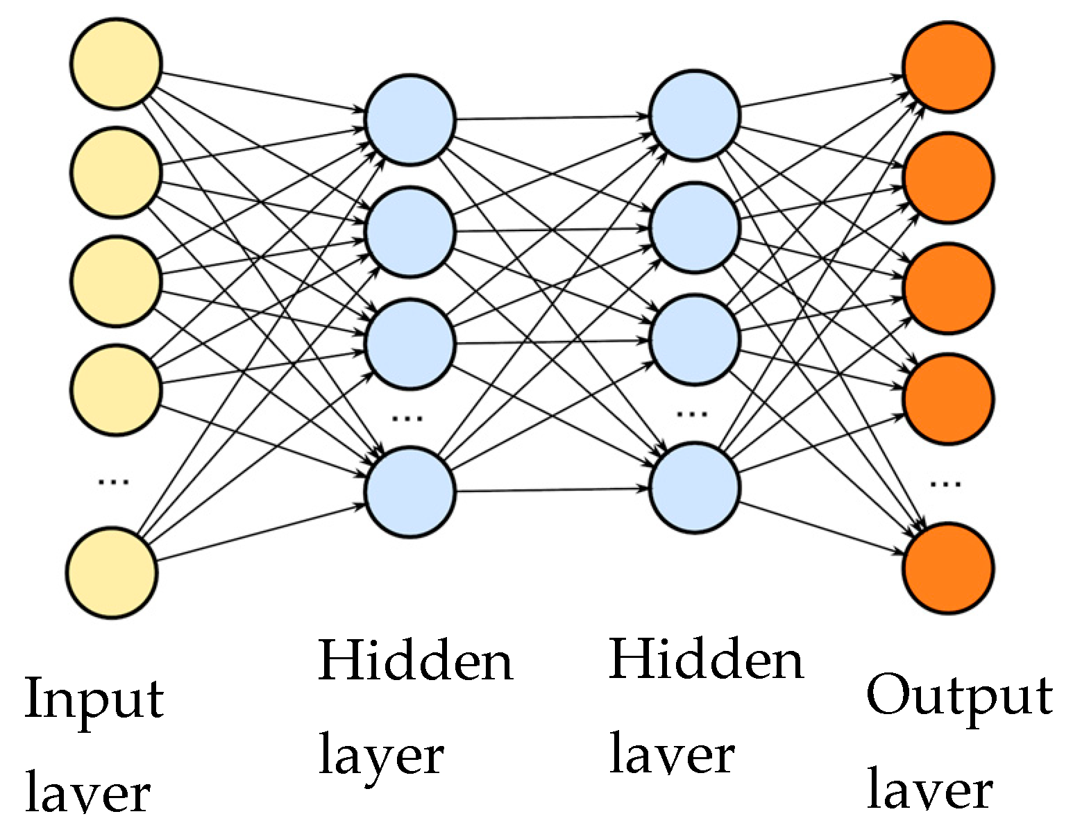
The proposed model for deep learning neural networks has four layers: one input layer, two hidden layers, and one output layer (Figure 5). There were 1856 training parameters in the first hidden layer, comprising architecture neurons that are entirely associated with 28 laser sensor inputs. A total of 4160 parameters were trained in the second hidden layer, including 64 neurons and 64 inputs from the first.

A programming program for the DQL algorithm is as follows (Algorithm 2):

Algorithm 2:

$\mathbf{Input}: \mathrm{data} X=\left(x_1,x_2,\mathrm{}\dots ,x_N\right)$, learning factor α, discount factor, epsilon-greedy policy $\in$, robot pose, safety constraints $\mathbf{Output}: Q\left(s,a;\theta \right)$, states’ s ∈ S, actions a ∈ A, weight θ Begin         Initialize replay memory $D$ to capacity N         $\mathrm{Initialize} Q\left(s,a;\theta \right)$ with random weights         $\mathrm{Initialize} Q\left(s,a^{\prime };{\theta }^{\prime }\right)$, with random weights for episode = 1, M do Randomly set the robots pose in the scenario Observe initial states of robots s for t = 1, T due to: $\mathrm{Select} \mathrm{an} \mathrm{action} a_t$    $\mathrm{With} \mathrm{probability}, \mathrm{select} \mathrm{a} \mathrm{random} \mathrm{action} a_t$   $\mathrm{Otherwise} \mathrm{select} a_t=argma{x}_{a^{\prime }}Q\left(s_t,a^{\prime };\theta \right)$   $\mathrm{Execute} \mathrm{action} a_t$$, \mathrm{observer} \mathrm{state} s_{t+1}$$, \mathrm{compute} \mathrm{reward} R_t$ $\mathrm{Store} \mathrm{training} \left(s_t,a_t,R_t,s_{t+1}\right)$ in relay memory EASY $\mathrm{Sample} \mathrm{random} \mathrm{minibatch} \mathrm{of} \mathrm{transition} \left(s_t,a_t,R_t,s_{t+1}\right)$ from EASY $\mathrm{Calculate} \mathrm{the} \mathrm{predicted} \mathrm{value} Q\left(s_j,a_j;\theta \right)$ Calculate the target value for each minibatch transition   $\mathrm{If} s_{t+1}$$\mathrm{is} \mathrm{the} \mathrm{terminal} \mathrm{state}, \mathrm{the} y_j=R_j$                     $\mathrm{Otherwise} y_j=R_j+\gamma {\max }_{{a^{\prime }}_j}{Q}^{\prime }\left({s^{\prime }}_j,{a^{\prime }}_j;{\theta }^{\prime }\right)$                     $\mathrm{Train} \mathrm{neural} \mathrm{networks} \mathrm{using} {(y_j-Q\left(s_j,a_j;\theta \right))}^2$ end for

The robot makes decisions and performs actions according to the Q-based (ε-greedy) policy. A mobile robot must successfully consider more than short-term gains over the long term. It is necessary to mention any prizes it might win in Class 1, Class 2, and Class L-1 future class. In addition, because the environment is unpredictable, the mobile robot can never be sure to receive the same reward the next time it carries out the same activities. Robots can diverge further as they advance in the future. Therefore, we employed a future discount reward in this study. The following formula is used to calculate the return on the future dilution factor at time t:

$$R_t=r_t+\gamma r_{t+1}+{\gamma }^2{r}_{t+2}+\mathrm{}\dots +{\gamma }^{T-t}{r}_T,0\le \gamma \le 1$$

(12)

where $r_t$ is the direct reward, and T is the time step at which the robot action ends; the further in the future the reward, the less the robot considers it.

The goal of the robot is to interact with the environment by choosing actions that maximize future rewards. We used a technique called experience replay, in which we record the robot’s experience at each time step, $e_t=\left(s_t,a_t,R_t,s_{t+1}\right)$, in a data set $D_t=\left\{e_1,\mathrm{}\dots ,e_t\right\}$, which is pooled over many learning cycles (episodes) at the end of the learning cycle into replay memory.

It is necessary to update the weights of neural networks. We first sampled random transitions from replay memory D with finite memory size N. For each given transformation, the algorithm performs the following steps:

-

Step 1: Transition through the neural network for the current state to obtain the predicted value Q(s_j, a_j; θ).

-

Step 2: If the transition sampled is a collision sample, then the evaluation for this pair ($s_j,a_j$) is directly set as the termination reward. Otherwise, forward neural networks are performed for the next state s’, the maximum overall network output is calculated, and the target for the action is computed using the Bellman equation (r + ${\max }_{a_j^{\prime }}{Q}^{\prime }\left(s_j^{\prime },a_j^{\prime };{\theta }^{\prime }\right)$). For all other activities, the target value is set to be the same as that initially returned in step 1.

-

Step 3: The Q-learning update algorithm uses the following loss function:

$$L\left(\theta \right)=\frac{1}{N}{\sum }_{i=1}^n{(y_j-Q\left(s_j,a_j;\theta \right))}^2$$

(13)

The neural network weights were changed using a loss function through backpropagation and stochastic gradient descent. The mobile robot stores the learned neural networks in its brain when the training is over and uses them for future testing and work.

4. Simulation and Experimental Results

This study proposes a DQL-based obstacle avoidance trajectory planning strategy for a mobile robot operating in an unexplored area using a LIDAR sensor. The LIDAR sensor acquires the distance value in the system and decides what steps to take next based solely on the distance of the obstacle to the mobile robot. Our proposed framework is depicted in Figure 6.

Our navigation framework consists of two main stages: (1) In the Offline stage, trajectories are sampled using the robot’s kinematic model. A 3D map structure is created around the robot by a LIDAR sensor and a hector SLAM algorithm. The voxels are categorized as “Priority” or “Support” based on their proximity to the nearest sampling point. (2) During the online stage, sensor data are translated into categorized voxels to compute occupancy values for each trajectory. The neural network generates a discrete action based on these observations. The online stage continues until a terminal state (goal or collision) is reached.

Action Space: In this paper, we utilize a 2D vector space to depict our actions as $a=\left[v \omega \right]\in R^2$ as we conduct simulations on a differential drive robot controlled by linear v and angular ω velocity commands.

Reward function: The reward function is calculation is Equation (12).

$$Reward=\{\begin{array}{c}{r}^{goal} if d_t^{target}<{\tau }^{target} \\ r^{fail} else if n_t>n^{\max step} or d_t^{obs}<{\tau }^{fail} \\ r_t^{step}=r_t^{target}+r_t^{step} else\end{array}$$

(14)

where:

$$r_t^{target}={\beta }^{target}\left( d_{t-\mathsf{\Delta }t}^{target}-d_t^{target}\right)$$

(15)

$$r_t^{step}=\frac{{\beta }^{target}}{n^{\max step}}$$

(16)

We set a positive reward goal $r^{target}$ for the robot when the mobile robot reaches the target. Suppose the episode ends by exceeding a threshold ${\tau }^{fail}$, reaching the closest obstacle’s distance value $d_t^{obs}$, or reaching the maximum number of steps $n^{max}$ per episode. In that case, we penalize it with a negative reward $r^{fail}$. To reduce the training time spent by the robot in inefficiently exploring its state space, we introduce a step reward function $r_t^{step}$ to evaluate states other than the end cases.

The step function target $r_t^{target}$ is calculated by finding the difference between the current and previous time steps’ target distance. This difference is then multiplied by the user-defined scalar beta target to adjust the reward/penalty weight on the navigation. Depending on the distance difference’s sign, the function penalizes or rewards the current state. The step function $r_t^{step}$ penalizes the robot for not reaching the goal. The penalty value μstep pen remains constant for each time and is determined by the user-defined scalar ${\beta }^{target}$ step and $n^{\max step}$. Including the previous action in observations helps the robot escape dead spots by compelling it to choose different activities. To address the potential issue of local minima, we introduce a mechanism to encourage exploration. By incorporating the previous action in the observations, we compel the robot to diversify its activities, thus mitigating the risk of getting stuck in unproductive states. This approach promotes a more adaptive and exploratory behavior, enabling the robot to navigate more effectively through complex environments. Moreover, using a user-defined scalar $\beta$ step pen and $n^{\max step}$ allows for fine-tuning the penalty for not reaching the goal, providing flexibility in adjusting the learning process to specific task requirements. Combining these strategies contributes to a more robust and efficient navigation system, enhancing the robot’s ability to overcome challenges and achieve its objectives.

In this process, the unnatural acceleration or deceleration actions of the system are required during resonance. The action value frequently fluctuates, physically shocks the robot, and reduces path performance. Therefore, the action values are returned to the input in the order of the network action after being held in memory.

In addition, reinforcement learning was simulated on the Robot Operating System and Gazebo simulator (ROS–GAZEBO), and the experiments were conducted on actual mobile robots by using scenarios and analyzing the experiment.

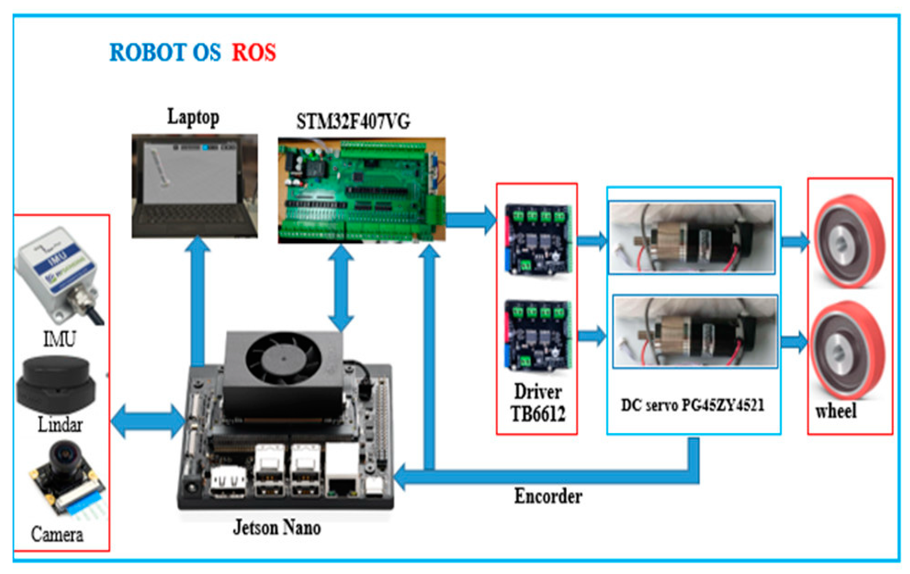
In this study, a mobile robot was experimentally built with specific specifications and a steel body size of 70 cm × 50 cm × 38 cm. Its 10 cm diameter wheels handle nearly any surface in the home. The two motor shafts hold 1200-tick encoders. This differential drive platform is comprehensive and can rotate in place. The wheels move only on one side, with two DC motors attached to the encoder. The robot was equipped with a Jetson Nano 4G embedded computer processor. ROS programming software specifications, motor encoder information, and other I/O via packets from the Jetson Nano 4G walker server all micro-control to the personal computer (PC) client and return control commands. Signals were obtained for power from the Linda 3600 A2 sensors, camera, and inertial measurement unit (IMU). ROS software provides library functions for navigation, path planning, obstacle avoidance, and many other robotic tasks. Figure 7 displays the experimental model of the mobile robot.

4.1. Set Status for a Mobile Robot

This state is an environment that observes and describes the current position of the robot. The state size is 28, with 24 values for the laser distance sensor, the distance to the target, and the angle to the target.

4.2. Set Action for a Mobile Robot

The robot could perform actions only in each state. The linear speed of the mobile robot in this situation was always 0.15 m/s. This is the act of determining the angular rate. The authors used a mobile robot model (Figure 8) that could only perform the five possible tasks listed in

Table 1. Action and angular velocity.

Action	Angular Velocity
0	−1.5
1	−0.75
2	0
3	0.75
4	1.5

.

4.3. Setup of a Reward for a Mobile Robot

The mobile robot performs an action in this state. It then receives a reward. Reward design is crucial to learning. Rewards can be either positive or negative. When the robot achieves its goal, it receives a sizeable positive compensation. When the robot collides with an obstacle, it receives a large negative reward.

4.4. Parameter Setting for the Controller

Parameter setting for the controller is listed in

Table 2. Action and angular velocity.

T	6000 (s)	Time step of one cycle
γ	0.99	The discount factor
α	25 × 10−5	Learning speed
ξ	1.0	Probability of choosing a random action
ξreduce	0.99	Reduction rate of epsilon. When a cycle ends, epsilon decreases
ξmin	0.05	Minimum stats of epsilon
Batch size	sixty-four	Activate a group of training templates
Train start	Sixty-four	Start of input training
Memory	106	Memory size

.

4.5. Simulation Results on ROS-GAZEBO

In this study, the control robot system created a scenario similar to that of a simulated factory in ROS-Gazebo to bridge the gap between the simulated environment and the natural world.

In this environment, various obstacles were built to test the proposed QL and DQL navigation algorithms. The territory includes walls, static blocks, mobile people, targets, and mobile robots. The mobile robot must reach the target while avoiding static and dynamic obstacles, as illustrated in Figure 9.

The training process for a robot can undergo several cycles. Each cycle ended when the robot acquired the target position, hit an obstacle in its path, or when the time for each cycle ended.

In this environment, various types of obstacles, including pedestrians, static blocks, and walls, were randomly placed to test the performance of the proposed mobile robot navigation algorithm. The task of the robot is to avoid static and dynamic barriers by maintaining a safe distance from them and reaching the target positions in the shortest distance and fastest time.

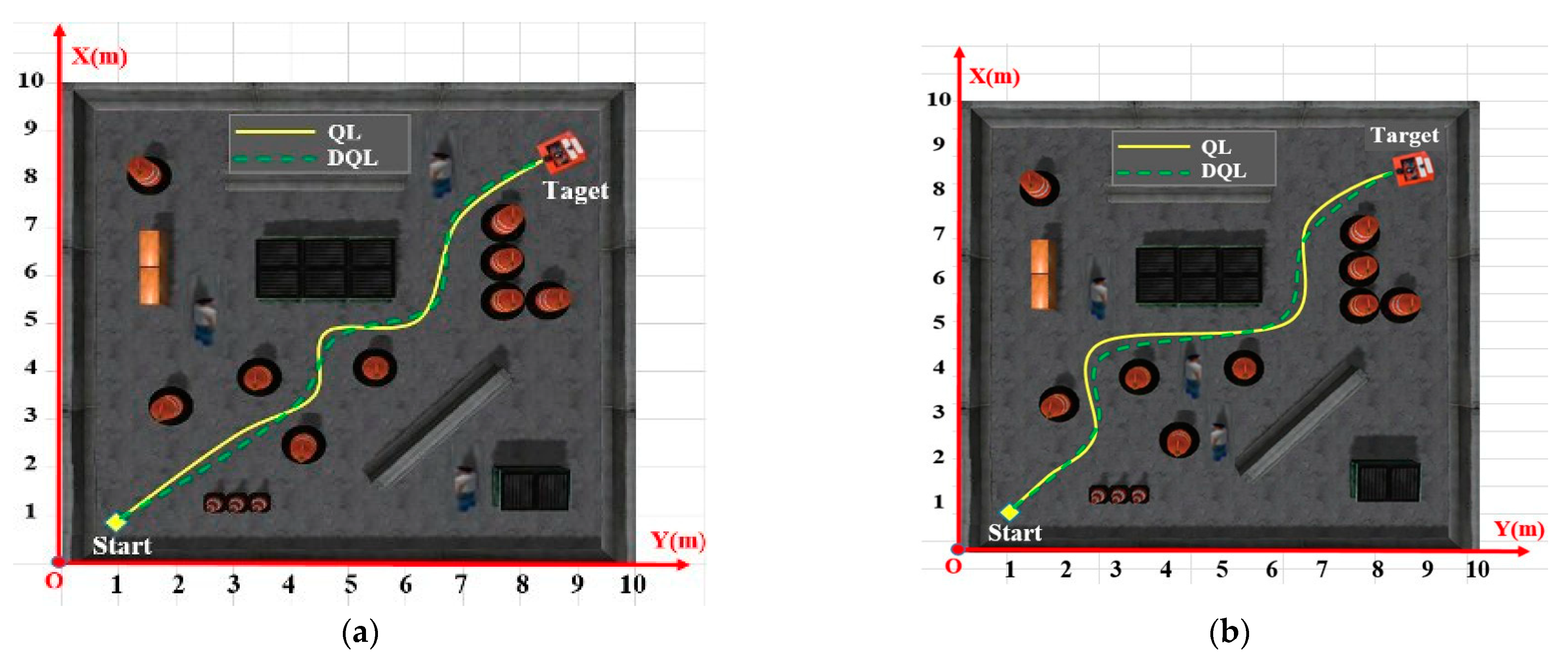
The path planning results of mobile robots using two algorithms, QL and DQL, in dynamic environments were assessed in this study. Figure 10 shows a realistic environment for path planning for a mobile robot, where the workspace is 12 m × 12 m with obstacles and the minimum distance between blocks is 0.6 m. For all tests, the robot starts from position (1, 1) and finds the path to the target (11, 11).

Table 3. Simulation results in ROS-GAZEBO.

No.	Algorithm	Case 1		Case 2
		Distance (m)	Run Time (s)	Distance (m)	Run Time (s)
1	QL	17.758	12.314	18.416	14.637
2	DQL	17.129	7.927	17.235	8.324

, below, presents the results.

The results in Table 3 show that both controllers effectively guide the mobile robot in planning the most efficient path. Specifically, with the DQL controller, the trajectory is enhanced, resulting in a shorter distance traveled, although the improvement is not considered significant. At the same time, the computational time needed to determine the optimal rotation and motion is notably improved. In the dynamic environment mirroring that of the QL algorithm in case 1, the distance covered is 17.758 m over 12.314 s. In contrast, with the DQL algorithm, the system covers a distance 0.629 m shorter in almost half the time, taking only 7.927 s. In case 2, the distance covered is 18.416 m over 14.637 s. Conversely, with the implementation of the DQL algorithm, the system covers a distance 1.181 m shorter in almost half the time, taking only 8.324 s. These findings suggest that the DQL algorithm produces superior outcomes compared to the QL algorithm.

4.6. Experiment Results

The experimental studies on robots with the two proposed algorithms involved many obstacles in this environment, including walls, tables, chairs, and students walking. The mobile robot must reach the target while avoiding the static and dynamic barriers (Figure 11). In this study, the robot was subjected to the following experimental cases:

Case 1: The actual environment for mobile robot path planning, where the workspace is a 4.5 m × 6.8 m robot club room with obstacles. The experimental study in Case 1 is presented in Figure 12.

Case 2: A mobile robot running down the hallway. The obstacles in this environment are pillars in the corridor and a cargo box that blocks the middle of the route. The distance from the starting point to the destination in a straight line (as the crow flies) is 20 m. The experimental study in Case 2 is presented in Figure 13.

Case 3: The mobile robot runs along the hallway with 20 kg of weight, as shown in Figure 13. The obstacles in this environment are pillars in the corridor and a cargo box that blocks the middle of the way. The experimental study in Case 3 is presented in Figure 14.

As shown in the Figure 12, Figure 13 and Figure 14 test results, the mobile robot starts at the door position (1, 1) and finds the path to the target (red, 5.5 m from the door). The experimental results of the two algorithms are listed in

Table 4. Simulation results in ROS–GAZEBO.

No.	Algorithm	Case 1
		Distance (m)	Run Time (s)
1	QL	6.271	72.132
	DQL	5.753	47.853
2	QL	6.314	74.097
	DQL	5.958	51.845
3	QL	6.264	72.124
	DQL	5.386	45.734
		Case 2
		Distance (m)	Run time (s)
1	QL	20.123	57.372
	DQL	21.235	32.735
2	QL	20.123	57.375
	DQL	21.235	33.738
3	QL	20.123	57.379
	DQL	19.235	30.735
		Case 3
		Distance (m)	Run time (s)
1	QL	27.682	92.132
	DQL	25.638	87.867
2	QL	27.682	92.132
	DQL	25.638	87.656
3	QL	27.682	92.132
	DQL	26.338	60.853

.

Based on the results presented in Table 4, it is evident from the experimental data that across all three cases, the DQL algorithm consistently outperforms the QL algorithm in the context of orbital planning for mobile robots, particularly concerning time efficiency. For instance, in Case 1, the DQL algorithm reduces the orbit length by 0.878 m and demonstrates a shorter duration of 26.390 s compared to the QL algorithm. Similarly, in Case 2, the DQL algorithm shortens the orbit by 0.88 m, with a reduced time of 26.644 s, in comparison to the QL algorithm. Finally, in Case 3, the DQL algorithm demonstrates a reduction of 1.344 m in orbit length and a shorter time of 31.279 s compared to the QL algorithm.

These outcomes strongly indicate the effectiveness of the DQL algorithm in trajectory planning for mobile robots within uncertain and dynamic environments. The DQL algorithm is adept at establishing an optimal trajectory and consistently invests more time in generating high-quality solutions. Furthermore, the execution time variability of the proposed DQL method increases as the number of barriers rises, highlighting its adaptability. In contrast, the DQL technique consistently delivers robust results within a short timeframe.

5. Conclusions

The deep Q-learning (DQL) algorithm is introduced in this study as a solution to create an optimal path for mobile robots in complex and dynamic environments. The algorithm helps the robot select the best action, speed up the learning process, find the ideal trajectory, and provide the Q table’s most favorable value for each action–state pair in a complex environment. The simulations and experiments show the proposed algorithm’s efficiency and superiority compared to the QL algorithm. Additional control functions such as classification, identification using image processing, voice control, and lane identification using intelligent control algorithms must be designed to improve the mobile robot’s trajectory further. This is the future research direction of the authors’ research group. Implementing these additional control functions will require a thorough understanding of the robot’s environment and the ability to adapt to changing conditions in real-time. Developing robust and reliable algorithms that can handle dynamic environments’ complexities and ensure mobile robots’ safety and efficiency is essential. Additionally, integrating advanced sensor technologies and machine learning algorithms will play a crucial role in enhancing the capabilities of mobile robots and enabling them to navigate complex and unpredictable environments with ease and precision. Furthermore, integrating advanced sensor technologies and machine learning algorithms will be pivotal in enhancing the capabilities of mobile robots. This integration will enable them to navigate complex and unpredictable environments quickly and precisely. Developing robust and reliable algorithms that can handle the complexities of dynamic environments and ensure the safety and efficiency of mobile robots is essential for their widespread adoption. As mobile robots become increasingly prevalent in various industries, the ability to adapt to changing conditions in real time and navigate through challenging environments will be crucial for their successful deployment.

References

1. Volos, C.K.; Kyprianidis, I.M.; Stouboulos, I.N. A chaotic path planning generator for autonomous mobile robots. Robots Auton. Syst. 2012, 60, 651–656. [Google Scholar] [CrossRef]
2. Châari, I.; Koubâa, A.; Trigui, S.; Bennaceur, H.; Ammar, A.; Al-Shalfan, K. SmartPATH: An efficient hybrid ACO-GA algorithm for solving the global path planning problem of mobile robots. Int. J. Adv. Robot. Syst. 2014, 11, 94. [Google Scholar] [CrossRef]
3. Gharajeh, M.S.; Jond, H.B. An intelligent approach for autonomous mobile robots path planning based on adaptive neuro-fuzzy inference system. Ain Shams Eng. J. 2021, 13, 101491. [Google Scholar] [CrossRef]
4. Vagale, A.; Oucheikh, R.; Bye, R.T.; Osen, O.L.; Fossen, T.I. Path planning and collision avoidance for autonomous surface vehicles I: A review. J. Mar. Sci. Technol. 2021, 26, 1292–1306. [Google Scholar] [CrossRef]
5. Zhang, C.; Zhou, L.; Li, Y.; Fan, Y. A dynamic path planning method for social robots in the home environment. Electronics 2020, 9, 1173. [Google Scholar] [CrossRef]
6. Yingqi, X.; Wei, S.; Wen, Z.; Jingqiao, L.; Qinhui, L.; Han, S. A real-time dynamic path planning method combining artificial potential field method and biased target RRT algorithm. J. Phys. Conf. Ser. 2021, 1905, 012015. [Google Scholar] [CrossRef]
7. Yang, B.; Yan, J.; Cai, Z.; Ding, Z.; Li, D.; Cao, Y.; Guo, L. A novel heuristic emergency path planning method based on vector grid map. ISPRS Int. J. Geo-Inf. 2021, 10, 370. [Google Scholar] [CrossRef]
8. Xiao, S.; Tan, X.; Wang, J. A simulated annealing algorithm and grid map-based UAV coverage path planning method for 3D reconstruction. Electronics 2021, 10, 853. [Google Scholar] [CrossRef]
9. Lin, T. A path planning method for mobile robot based on A and antcolony algorithms. J. Innov. Soc. Sci. Res. 2020, 7, 157–162. [Google Scholar]
10. Guo, J.; Liu, L.; Liu, Q.; Qu, Y. An Improvement of D* Algorithm for Mobile Robot Path Planning in Partial Unknown Environment. In Proceedings of the 2009 Second International Conference on Intelligent Computation Technology and Automation, Changsha, China, 10–11 October 2009; ISBN 978-0-7695-3804-4. [Google Scholar] [CrossRef]
11. Lai, X.; Wu, D.; Wu, D.; Li, J.H.; Yu, H. Enhanced DWA algorithm for local path planning of mobile robot. Ind. Robot. Int. J. Robot. Res. Appl. 2022, 50, 186–194. [Google Scholar] [CrossRef]
12. Zong, C.; Han, X.; Zhang, D.; Liu, Y.; Zhao, W.; Sun, M. Research on local path planning based on improved RRT algorithm. Proc. Inst. Mech. Eng. Part D J. Automob. Eng. 2021, 235, 2086–2100. [Google Scholar] [CrossRef]
13. Tsai, C.C.; Huang, H.C.; Chan, C.K. Parallel elite genetic algorithm and its application to global path planning for autonomous robot navigation. IEEE Trans. Ind. Electron. 2011, 58, 4813–4821. [Google Scholar] [CrossRef]
14. Saska, M.; Macăs, M.; Přeučil, L.; Lhotská, L. Robot path planning using particle swarm optimization of Ferguson splines. In Proceedings of the IEEE International Conference on Emerging Technologies and Factory Automation (ETFA), Diplomat Hotel Prague, Czech Republic, 20–22 September 2006; IEEE Press: New York, NY, USA, 2006; pp. 833–839. [Google Scholar]
15. Raja, P.; Pugazhenthi, S. On-line path planning for mobile robots in dynamic environments. Neural Netw. World 2012, 22, 67–83. [Google Scholar] [CrossRef]
16. Thuong, T.T.; Ha, V.T. Adaptive Control for Mobile Robots Based on Inteligent Controller. J. Appl. Sci. Eng. 2023, 27, 2481–2487. [Google Scholar]
17. Thuong, T.T.; Ha, V.T.; Truc, L.N. Intelligent Control for Mobile Robots Based on Fuzzy Logic Controller. In The International Conference on Intelligent Systems & Networks; Springer: Singapore, 2023; pp. 566–573. [Google Scholar]
18. Chen, X.; Kong, Y.; Fang, X.; Wu, Q. A fast two-stage ACO algorithm for robotic path planning. Neural Comput. Appl. 2013, 22, 313–319. [Google Scholar] [CrossRef]
19. Purcaru, C.; Precup, R.E.; Iercan, D.; Fedorovici, L.-O.; David, R.-C.; Dragan, F. Optimal robot path planning using gravitational search algorithm. Int. J. Artif. Intell. 2013, 10, 1–20. [Google Scholar]
20. Li, P.; Duan, H.B. Path planning of unmanned aerial vehicle based on improved gravitational search algorithm. Sci. China Technol. Sci. 2012, 55, 2712–2719. [Google Scholar] [CrossRef]
21. Duan, H.B.; Qiao, P.X. Pigeon-inspired optimization: A new swarm intelligence optimizer for air robot path planning. Int. J. Intell. Comput. Cybern. 2014, 7, 24–37. [Google Scholar] [CrossRef]
22. Liu, J.; Wang, Q.; He, C.; Jaffrès-Runser, K.; Xu, Y.; Li, Z.; Xu, Y. QMR:Q-learning based Multi-objective optimization Routing protocol for Flying Ad Hoc Networks. Comput. Commun. 2019, 150, 304–316. [Google Scholar] [CrossRef]
23. Low, E.S.; Ong, P.; Cheah, K.C. Solving the optimal path planning of a mobile robot using improved Q-learning. Robot. Auton. Syst. 2019, 115, 143–161. [Google Scholar] [CrossRef]
24. Luviano, D.; Yu, W. Continuous-time path planning for multi-agents with fuzzy reinforcement learning. J. Intell. Fuzzy Syst. 2017, 33, 491–501. [Google Scholar] [CrossRef]
25. Qu, C.; Gai, W.; Zhong, M.; Zhang, J. A novel reinforcement learning based gray wolf optimizer algorithm for un-manned aerial vehicles (UAVs) path planning. Appl. Soft Comput. 2020, 89, 106099. [Google Scholar] [CrossRef]
26. Watkins, C.J.; Dayan, P. Q-learning. Mach. Learn. 1992, 8, 279–292. [Google Scholar] [CrossRef]
27. Jaradat, M.A.K.; Al-Rousan, M.; Quadan, L. Reinforcement based mobile robot navigation in dynamic environment. Robot. Comput. Manuf. 2011, 27, 135–149. [Google Scholar] [CrossRef]
28. Ganapathy, V.; Yun, S.C.; Joe, H.K. Neural Q-learning controller for mobile robot. In Proceedings of the 2009 IEEE/ASME International Conference on Advanced Intelligent Mechatronics, Singapore, 14–17 July 2009; pp. 863–868. [Google Scholar]
29. Oh, C.H.; Nakashima, T.; Ishibuchi, H. Initialization of Q-values by fuzzy rules for hastening Qlearning. In Proceedings of the 1998 IEEE International Joint Conference on Neural Networks Proceedings, IEEE World Congress on Computational Intelligence (Cat. No. 98CH36227), Anchorage, AK, USA, 4–9 May 1998; Volume 3, pp. 2051–2056. [Google Scholar]
30. Jiang, J.; Xin, J. Path planning of a mobile robot in a free-space environment using Q-learning. Prog. Artif. Intell. 2019, 8, 133–142. [Google Scholar] [CrossRef]
31. Wang, Y.-H.; Li, T.-H.S.; Lin, C.-J. Backward Q-learning: The combination of Sarsa algorithm and Q-learning. Eng. Appl. Artif. Intell. 2013, 26, 2184–2193. [Google Scholar] [CrossRef]
32. Kdas, P.; Mandhata, S.C.; Behera, H.S.; Patro, S.N. An Improved Q-learning Algorithm for Path-Planning of a Mobile Robot. Int. J. Comput. Appl. 2012, 51, 40–46. [Google Scholar] [CrossRef]
33. Goswami, I.; Das, P.K.; Konar, A.; Janarthanan, R. Extended Q-learning algorithm for pathplanning of a mobile robot. In Proceedings of the Asia-Pacific Conference on Simulated Evolution and Learning, IIT Kanpur, India, 1–4 December 2010; Springer: Berlin/Heidelberg, Berlin, 2010; pp. 379–383. [Google Scholar]
Figure 1. Regarding obstacle estimation for route planning, the following should be listed: (a) a description of the 3D modeling of indoor environments; (b) a description of the 3D modeling of an indoor room; (c) a description of a binary map of the environment; (d) a description of the approximation of the obstacles by rectangles; (e) a description of the binary environment.
Actuators 13 00026 g001aActuators 13 00026 g001b
Figure 2. Q-learning algorithm.
Actuators 13 00026 g002
Figure 3. The table of Q parameters according to the state–action matrix.
Actuators 13 00026 g003
Figure 4. Deep Q-learning in Q value assessment.
Actuators 13 00026 g004
Figure 5. Architectural model.
Actuators 13 00026 g005
Figure 6. Robot Operating System (ROS) model.
Actuators 13 00026 g006
Figure 7. In the diagram, 0 is the left (−90°), 1 is the left front (−45°), 2 is the front (0°), 3 is the right front (45°), and 4 is the right (90°); a mobile robot’s actions are directed.
Actuators 13 00026 g007
Figure 8. Structure diagram of the hardware control mobile robot.
Actuators 13 00026 g008
Figure 9. Path planning simulation environment for mobile robots in ROS-Gazebo.
Actuators 13 00026 g009
Figure 10. Path planning results of mobile robot using two algorithms, QL and DQL, in a dynamic environment; they should be listed as (a) Case 1 and (b) Case 2.
Actuators 13 00026 g010
Figure 11. Realistic environment of the robot club room.
Actuators 13 00026 g011
Figure 12. Experimental image of the mobile robot movement room.
Actuators 13 00026 g012
Figure 13. Experimental image of the mobile robot movement room with a robot running along the hallway.
Actuators 13 00026 g013
Figure 14. Experimental image of the mobile robot movement room with a robot running along the hallway with 20 kg of weight.
Actuators 13 00026 g014