Abstract
Ultra-precise actuation at extremely low speeds over a broad range is a major challenge for advanced manufacturing. A novel two-axis differential micro-feed system (TDMS) has been proposed recently to overcome the low-speed crawling of the worktable. However, due to the diversity of the force states of the TDMS, the methods for identification identifyingof friction parameters traditionally (like the all -components identification method, ACIM) didn’t did not perform well. And many studies on the performance of the pre-sliding phase of the TDMS are missing. Therefore, a novel whole-system identification method (WSIM) based on the TDMS was proposed in this paper to precisely identify the friction parameters under different states of motion. The generalized Maxwell sliding (GMS) friction model was also applied to improve the accurate description of the pre-sliding. A novel corrected Stribeck curve based on the TDMS (TDMSSC) was proposed under the uniqueness of the TDMS structure. Control experiments showedn that the WSIM has higher precision and stability rather thancompared torather than the ACIM, and the correction of the Stribeck curve for the TDMS makes a contribution to the performance. This method significantly improves the accuracy and stability of the machine tool drive system.
1. Introduction
Numerous unique architectures for micro-displacement actuators have been proposed as a result of the growing demand for ultra-precision machine tools [1,2,3]. Feng [4,5] introduced a novel two-axis differential micro-feed system (TDMS), which addressed the issue of the nonlinear friction-induced creeping of traditional drive-feed systems at low speeds when it is wais used to drive the machine tool. Two permanent -magnet synchronous motors (PMSMs) are used in the TDMS to drive the screw and nut, as seen in Figure 1. The worktable can run at a very low pace by superimposing the two transmission structures with two rotational movements in the same rotation direction and similar rates [6]. The nonlinear disturbance from the ball screw is substantially less than the conventional drive feed system (CDFS) since the screw and nut operate at high speeds [7,8].
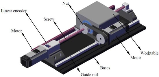
Figure 1.
Structure diagram of the TDMS.
The creation of an accurate friction model [9,10] and the identification of friction characteristics [11] are crucial to the execution of friction compensation control [12,13,14]. The choice of the friction model depends on a variety of different physical characteristics and operational circumstances [15] because friction is complex and nonlinear [16]. To identify the parameters for the TDMS, the LuGre friction model [17] and feed-forward friction compensation [18] were used, but the LuGre model fails to effectively capture the nonlocal memory phenomenon [19]. In contrast to the experience-based friction model discussed above, the general Maxwell Sliding sliding [20] model was used from a microscopic perspective to explain the observed macroscopic friction behavior, describe the hysteresis curve using the Maxwell sliding model, and address the problems above. It designs extra parameters to characterize the friction lag effect [21,22].
The force conditions of the TDMS in various working states are not taken into consideration for the all-components friction model (ACIM) [23,24], limiting the friction model parameters’ reliability of identification. When the worktable runs or stops, the screw and nut are at a different speed or the same speed. So even if the whole -component-based identification method (ACIM) proposed by Feng [25] is accurate for each structure, the identification parameters are unknown since this approach does not account for the force conditions in various motion states caused by the structural peculiarity of the TDMS. Although Feng [26] discovered the impact of various base speeds on friction characteristics, he overlooked the impact of various operating conditions on the outcomes of the identification process.
In light of these issues, the GMS model is applied to precisely characterize the system, along with the nonlocal memory, which has higher precision than that with the LuGre model. In addition, a unique, simpler, and more accurate method for identifying the friction model parameters based on the TDMS in various motion states was proposed, with better performance than that of the ACIM.
This essay is structured as follows: The friction modeling and dynamic modeling of the TDMS based on the GMS model are covered in the second section. The third section suggests a novel parameter identification approach for the TDMS. A full-closed-loop friction compensation control mechanism is designed in the fourth section. The experiment is carried out, and the fifth section discusses the findings. The performances of the systems based on the ACIM and WSIM simulation models and the GMS and LuGre friction models are compared. The final section of this study provides a summary of its findings.
2. Friction Analysis and Dynamics Modeling for TDMS
2.1. The GMS Friction Model
The GMS friction model is a model with physical imaginary significance designed from the microscopic mechanism [27]. It combines many friction units in parallel into an overall friction model. Each friction unit consists of a massless slider and a spring. The slider remains still when the spring deformation is less than its maximum elastic deformation. Sliding occurs when the spring deformation is greater than the maximum elastic deformation. The stiffness of a system at a certain position is the sum of the stiffness of all the stationary slides in the current position.
The friction force of the whole sliding model is equal to the sum of the friction force of each friction unit and viscous friction:
is the viscous friction coefficient, is the number of friction units, and is the speed of the object. The meanings of the unspecified variables in this section and the fourth section are shown in Table 1. When the system is in the sliding region, according to the GMS model [23], the sum of the friction force of each friction unit mentioned above is presented as
The transformation form is
The represents the Stribeck curve. The speed of the friction force converging to the Stribeck curve in the sliding region is determined by the lag coefficient . According to the formulation of the LuGre model,
With the increase in the speed, the value of the Stribeck curve decreases. The maximum of it is , and the minimum of it is the Coulomb friction , in which is the Stribeck speed and is the Stribeck factor.
2.2. Friction Modeling of the TDMS
Based on the above description of the GMS model in the pre-sliding and sliding states, the friction model expressions for the driving shaft (screw and nut) and worktable of the TDMS are expressed as follows. The meanings of the parameters are shown in Table 1.

Table 1.
Parameters used in model of the TDMS.
Table 1.
Parameters used in model of the TDMS.
| Parameters | Meaning |
| friction torque of screw and nut | |
| friction moment generated by each friction unit of the screw and nut | |
| viscous friction coefficient of the screw and nut | |
| speed of the screw and nut | |
| Coulomb friction torque of the screw and nut | |
| maximum static friction torque of the screw and nut | |
| Stribeck speed of the screw and nut | |
| friction force between the worktable and guide rail | |
| number of friction units of the screw, nut and workbench | |
| friction force generated by the i-th friction unit of the workbench | |
| viscous friction coefficient of the worktable | |
| relative speed between the workbench and guide rail | |
| stiffness coefficient of the i-th friction unit of the screw, nut and workbench | |
| spring deformation of the i-th friction unit of the screw, nut and workbench | |
| maximum spring deformation of the friction unit of the screw, nut and workbench | |
| lag parameters of the screw, nut and workbench | |
| weight coefficient of the i-th friction unit of the screw, nut and workbench | |
| Coulomb friction of the workbench | |
| maximum static friction force of the workbench | |
| Stribeck speed of the workbench | |
| Stribeck factor of the screw, nut and workbench |
2.2.1. Driving Shaft
Below are the dynamic equations and friction model of the drive shaft.
2.2.2. Worktable
Below are the dynamic equations and friction model of the worktable.
2.3. Dynamics Modeling of TDMS
When the two axes drive at the same rotation, avoiding low speed, the workbench can be fed with a small relative speed. The friction forces between the screw and ball and nut and ball are represented by , where represents the agent of force and represents the patient of force. The dynamic model of the TDMS is shown in Figure 2.
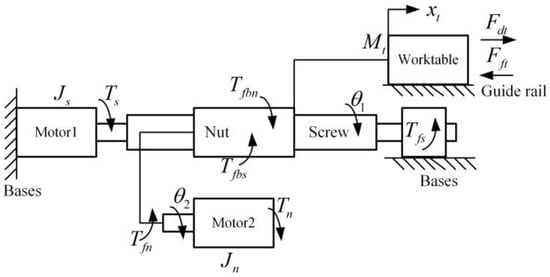
Figure 2.
Dynamic model of the TDMS.
When the screw and nut motor rotate clockwise, the screw speed is set to positive, while the nut speed is set negative. According to the figure above and Newton’s second theorem, the dynamic equation of the TDMS is presented as follows:
If the screw is the driving shaft,
If the nut is the driving shaft,
where represents the output torque of the screw and nut motor. represents the friction torque of the screw and nut. represents the equivalent driving torque to the workbench. represents the moment of inertia of the screw and nut, and represents the equivalent friction torque at the screw and nut. When the screw speed is greater than the nut speed, decelerates the screw and accelerates the nut, and reverse force is applied when the nut’s speed is greater than the screw.
According to the displacement characteristics of the TDMS, the bench displacement is , where is the conversion ratio of the rotational motion to straight motion. Then, , and the ratio of straight motion to rotational motion is represented as . The original form of is the equivalent driving force .
3. A Novel Identification Method of Friction Parameters for TDMS
When the screw and nut move in the same speed and direction, the worktable remains static. The ball is not affected by sliding friction. The driving motors just needs to overcome the friction and the inertia of the driving shaft, respectively. Since the shaft is not required to move the workbench, its pressure is minimal. This is shown in Figure 3.
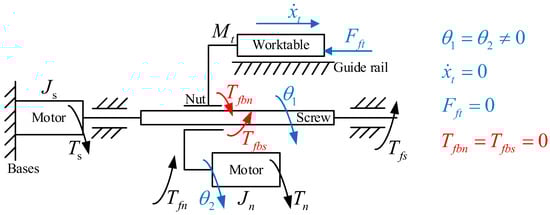
Figure 3.
Dynamic model of the TDMS when the screw and nut are in the same speed and direction.
When the screw is the driving shaft, the motor of the screw is intended to overcome friction not only at the driving shaft but also at the screw–nut pair. The friction between the workbench and guide rail must also be overcome by the screw motor. The axial pressure at the two driving axes differs significantly from the state at the same speed, and this is an important point to note. This is shown in Figure 4.
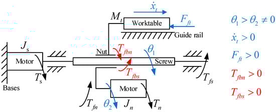
Figure 4.
Dynamic model of the TDMS when the screw is driving shaft.
When the nut is the driving shaft, it is intended that the motor of the nut overcomes friction not only at the driving shaft but also at the screw–nut pair. The friction between the workbench and guide rail must also be overcome by the nut motor. This is shown in Figure 5.
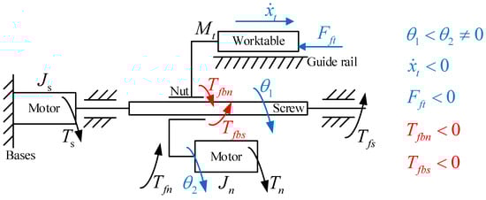
Figure 5.
Dynamic model of the TDMS when the nut is driving shaft.
In conclusion, the two-axis co-speed mode and two-axis differential-speed mode (including a single drive) should be applied to categorize the identification procedure, respectively. The reason for distinguishing between these two cases is the difference in axial pressure on the drive shaft, which is small at the same speed and large at different speeds. This originally resulted from friction between the worktable and guide rail being present or absent. The friction between the workbench and the guide rail causes the ball’s axial pressure at the screw–nut pair when there is a relative rotating speed between the screw and nut.
Whatever screw or nut is the driving shaft, a significant amount of reverse axial pressure (or tension) will be placed on another one. The friction at the ball–screw pair and between the worktable and rail in the TDMS is caused by the speed difference between the screw and nut motors because the amount of friction force is directly proportional to the pressure in addition to the pretension force. Therefore, the whole-system identification method (WSIM) rather than the all-components identification method (ACIM) should be used to identify the parameters for the TMDS under the two conditions of two-axis co-speed and two-axis differential speed.
As shown in Figure 6, the process of the identification of parameters is divided into four steps. In the first step, four parameters of the Stribeck curve and the viscous friction coefficient are identified via the torque–speed curve in the sliding stage when the two axes drive at the same speed. The second step is to identify the stiffness coefficient and the weight coefficient of the friction unit using the torque–position curve in the pre-sliding stage and select the appropriate lag parameter to make the friction force converge to the Stribeck curve quickly. The third and fourth period of identification when the two axes drive at different speeds is similar to the above two periods, in addition to including the identification of the worktable’s parameters.
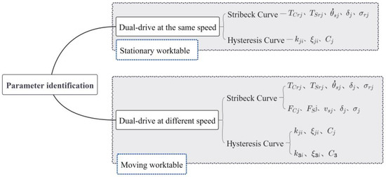
Figure 6.
Process diagram of parameter identification for TDMS.
4. Full Closed-Loop Friction Compensation
Let the target position of the screw and nut be and the tracking error be . The target position of the workbench is , and the tracking error is . The positions of both the screw and nut will affect the position of the workbench, . The displacement tracking error of the bench includes not only the displacement tracking error of the screw and the nut but also the fit clearance caused by the gap between the ball, screw and nut, i.e.,
Compensate the error to the screw with less inertia:
According to the accurate identification of the friction model parameters, the input of the drive motor of the screw and nut can be obtained, respectively:
A block diagram of the feed-forward friction compensation control based on the PID controller is shown in Figure 7.
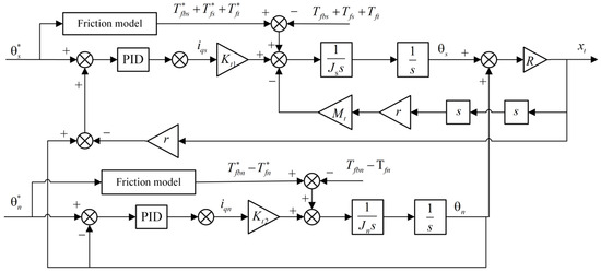
Figure 7.
Block diagram of PID with feed-forward friction compensation of full closed-loop control.
5. Experiments and Results
5.1. Equipment
Figure 8a,b display a schematic representation and shots of the experimental instrument. A ball screw (DIR 1605, THK) with a 16 mm diameter is inserted in the feed drive, which has a stroke of 280 mm. Two PMSMs (Panasonic MHMF042LV2M) with a combined rated power of 400 W and a rated torque of 1.27 Nm are used to drive the ball screw. The synchronous servo driver (Panasonic MBDLT25BF), which connects to the motor via a superior resolution rotary encoder (23 bits) and offers motor position feedback, uses the EtherCAT protocol to interface to the industrial control computer (ICC).
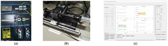
Figure 8.
Experiment equipment: (a) control circuits; (b) the TDMS; (c) ICC.
The worktable position is measured using a raster ruler with a 10 nm precision scale (KEYENCE GVS 600T), which is connected to the screw servo driver. The external sensor monitoring function of the screw servo driver is activated to read the raster ruler pulse data for fully closed-loop control at the ICC. The control software is created in a Windows 10+VS environment in the ICC, and KRMotion’s secondary development is carried out there using the process data object (PDO) function to read motor position, speed, torque and external raster ruler data directly. The control period is set to 250 us.
Based on the German Kithara real-time suite (KRTS), KRMotion is a real-time motion controller created by the Shandong E-Code firm. Figure 8c depicts the ICC software’s user interface. Table 2 displays the particular characteristics of the experimental apparatus.
Table 2.
Experimental equipment parameters.
5.2. The Identification of the Friction Parameters
5.2.1. Identification of Friction Model in Two-Axis Co-Speed Mode
Static Friction Parameter Identification
Four parameters of the Stribeck curve and the viscous coefficient were identified. When the two axes run in the same direction and equal speed, the worktable is in a quasi-stationary state, and there is no sliding friction between the screw and nut. The dynamic equation is expressed as
The friction force remains unchanged in the steady stage; that is, . According to Equation (3), , so
The output is the speed of the driving shaft and the input is the current . MATLAB was used to fit and identify the parameters and .
Figure 9 shows the static friction characteristics of the screw and nut in a two-axis co-speed driving mode. The identification results of clockwise and counterclockwise rotation are shown in Table 3.
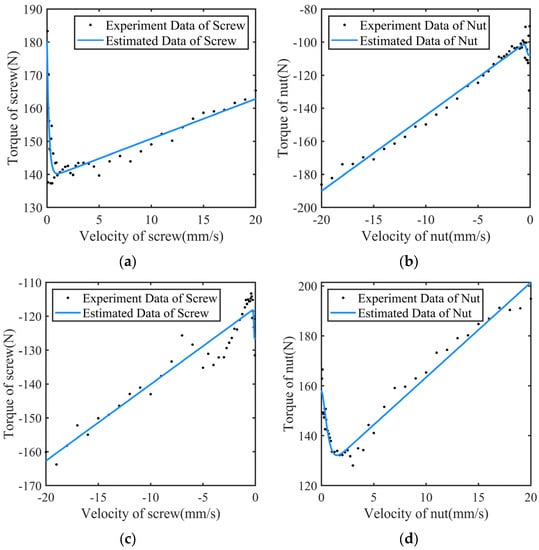
Figure 9.
Static friction characteristics in two-axis co-speed driving mode: (a) friction characteristics of screw when rotate clockwise; (b) friction characteristics of nut when rotated clockwise; (c) friction characteristics of screw when rotated counterclockwise; (d) friction characteristics of nut when rotated counterclockwise.
Table 3.
Identification of static frictional parameters in two-axis co-speed mode.
Dynamic Friction Parameter Identification
The identification of the stiffness coefficient and the weight coefficient adopts the method of [28]. The two driving axes rotate with a micro-speed in the same direction and reciprocate within several microns to create the pre-sliding state, as shown in Figure 10.
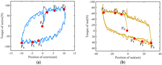
Figure 10.
Dynamic friction characteristics in two-axis co-speed driving mode, which represents the frictional properties of the pre-slip region during round trip: (a) friction characteristics of screw; (b) friction characteristics of nut.
During the periodic motion, the friction force is approximately linear to the displacement of hysteresis. The ascending segment of the hysteresis curve can be divided into four states, namely, from the initial state to the inverted state . The number of friction units , assuming that the critical points when rotating counterclockwise are . The corresponding stiffness coefficient can be obtained according to the torque corresponding to the critical point. The three state critical points when the two axes rotate counterclockwise are .
Similarly, in the hysteresis curve of the 30 μm stroke of the nut, the three critical points in the clockwise rotation are , and the three critical points for the counterclockwise rotation are . The parameter meets
where is the relative displacement from the breaking point of the i-th unit to the initial position. The system is simulated in Simulink using Equation (2) to minimize the error between the model-predicted displacement and the actual displacement. The result is shown in Table 4.
Table 4.
Identification of dynamic frictional parameters in two-axis co-speed mode.
5.2.2. Identification of Friction Parameters in Two-Axis Differential-Speed Mode
Static Friction Parameter Identification
A feature of the TDMS compared to the CDFS is to obtain the low-speed motion composed of the high-speed motions of the two driving shafts. By first accelerating the screw and nut to the same base speed, retaining the nut at that speed while gradually raising or reducing the speed of the screw, the workbench can be moved. Take the screw as an example of the driving shaft. This technique significantly increases accuracy by preventing the motor’s hysteresis effect.
By increasing it from zero to greater, the impact of various base speeds on the identification outcomes of friction characteristics is examined. As previously mentioned, there is a big difference between the axial pressure on the screw and nut in the differential drive mode and same-speed mode. Integrate the friction at the nut motor and screw–nut pair as a friction linked to the speed of the worktable for the nut motor and the friction at the screw motor, screw–nut pair and guide rail as a friction related to the speed of the worktable for the screw motor. Consider the external friction of the two rotating axes as one, expressed as
The friction–velocity curves of the screw and nut at various base speeds are shown in Figure 11, clockwise. The specific changes are initially described by the second-order Fourier function to avoid fitting mistakes. Figure 11a demonstrates how the curves match the Stribeck curve’s general trend. This further supports the appropriateness of considering the external disturbance of the entire system to be changing due to the Stribeck effect. The black curve illustrates how the external friction of the screw motor changes when the speed of the nut motor is zero in Figure 11b. The screw gradually changes from boundary friction to mixing friction to fluid friction when the speed is increased. When the nut is stationary and its speed is between −0.1 mm/s and −0.5 mm/s, the friction force varies across the curve. The boundary friction of the curve becomes unnoticeable, if it does not completely disappear, until the nut motor’s rotation speed hits −0.6 mm/s. It demonstrates how much better the dual-drive system is than the conventional single-drive system.
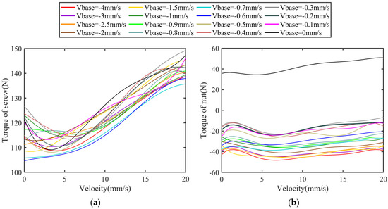
Figure 11.
Static friction characteristics in two-axis differential driving mode clockwise: (a) friction characteristics of screw; (b) friction characteristics of nut.
It is intended that the screw and nut first transition to the condition where the workbench is still and the screw and nut are at the base speed when the base speed is not zero. The screw can then be turned faster or slower, but because the motor has already been in a rotating state (with fluid friction), it is not necessary for it to also be in a static state to overcome boundary friction.
As can be seen from Equation (11), when the nut is still, the friction force from the ball makes a positive contribution on the nut, and there is no friction at the driving shaft of the nut. Therefore, the integrated friction force of the nut is positive. When , the ball will perform positive work on the nut. The frictional–velocity curve of the nut at low velocity differences conforms to the Stribeck curve.
The viscosity coefficient and velocity product are the main factors at play when the nut enters the fluid friction. The pressure differential between the screw–nut pairs rises with a second power of speed as the speed difference widens [29]. That is, the ball’s positive friction force on the nut increases more quickly than the driving shaft’s negative friction force. As a result, friction increases first and then reduces. By generally translating proportionally to the increase in base velocity, the friction curve at various base speeds can be produced. Therefore, and can be regarded as functions of a base speed and a quadratic term of the speed can be added, expressed as follows:
where represents the coefficient related to the change in friction force caused by the ball centrifugal force. The Coulomb force and separation force of the screw at a different speed are greater than those at the same speed, as shown in Figure 11a and the same speed curve. This demonstrates that the results made above on various driving modes are accurate. The Coulomb and separation forces of the nut, however, are lower than those rotating at a similar speed. This is due to the fact that the friction created by the ball when the screw serves as the driving shaft helps the nut rotate.
Figure 12 shows the friction–speed curves of the screw and nut in a differential-speed driving mode counterclockwise. The principle of the curves is similar to the clockwise rotation, which will not be repeated here. Because the change in the friction parameters of the screw is slight at different base speeds, the friction parameters at the base speed of 4 mm/s can be picked. The friction model parameters of the nut can be identified separately according to the friction models at different base speeds and finally synthesize the function about the velocity. The identification results are shown in Table 5.
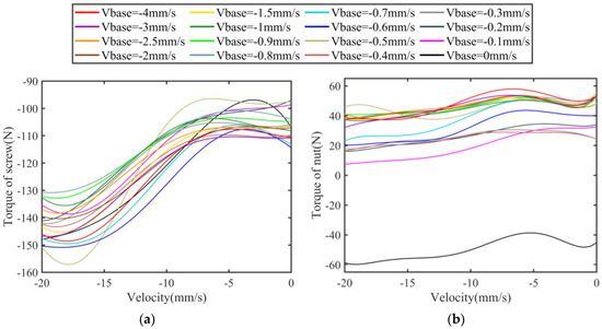
Figure 12.
Static friction characteristics in two-axis differentialdriving mode counterclockwise: (a) friction characteristics of screw; (b) friction characteristics of nut.
Table 5.
Identification of static frictional parameters in two-axis differential-speed mode.
Dynamic Friction Parameter Identification
To identify the dynamic friction parameters of the system, let the nut remain still and the screw reciprocate within microns. The output torque of the screw motor is the friction torque corresponding to different positions, as shown in Figure 13. The result is shown in Table 6.
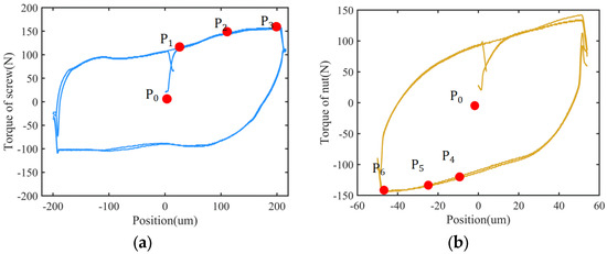
Figure 13.
Dynamic friction characteristics in two-axis differential speed driving mode, which represents the frictional properties of the pre-slip region during round trip: (a) friction characteristics of screw; (b) friction characteristics of nut.
Table 6.
Identification of dynamic frictional parameters in two-axis differential-speed mode.
5.3. Nonlocal Memory in the Hysteresis Curve with Different Friction Models
In order to compare the GMS and the LuGre friction model in describing nonlocal memory phenomena in the TDMS, the system was run at the two-axis co-speed mode of 3 μm/s and different-speed mode of 1 μm/s. Figure 14 is the position–time curve, and the corresponding hysteresis curves are shown in Figure 15 and Figure 16. Figure 15 is the hysteresis curve of the screw and nut under the same speed, and Figure 16 is the hysteresis curve of the screw for actual measurements and estimated curves with the LuGre and GMS model under different speeds.
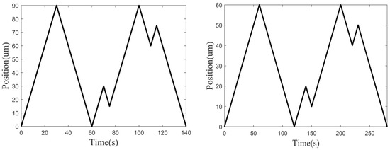
Figure 14.
Command displacement–time diagram during the nonlocal memory experiment.
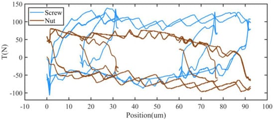
Figure 15.
Nonlocal memory phenomenon of screw and nut in two-axis co-speed driving mode.
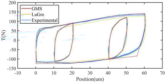
Figure 16.
Nonlocal memory of screw at two-axis differential speeds with different friction models.
It can be seen that the torque of screw and nut will grow up and down randomly. This is due to the fact that the workbench hysteresis is always caused by a little speed difference between the two axes when two motors are operating simultaneously. Axial pressure and friction will be created in the screw–nut pairs when the workbench moves. The screw starts to slow down the acceleration due to the pressure, while the nut starts to speed up the acceleration, increasing the difference in speed between the two axes, if the table is going forward (the screw is turning clockwise). But the speed will not change too quickly due to the ball’s previously indicated working effect on the screw and nut. When the speed error is big enough, the actuator immediately applies a reverse torque according to the feedback signal, and the whole system begins to repeat the above process in reverse.
It can be seen that both models can describe the overall trend of the hysteresis curve well, but the curve of LuGre is smoother than that of GMS in the case of unidirectional movement, which more appropriately describes the unidirectional movement hysteresis curve of the workbench. This is because the friction contact surface is only divided into three friction units, but in fact there are countless friction units, so the trend of the hysteresis curve can be described more accurately by increasing the number of friction units. Article [30] shows that 6 to 7 friction units are the optimal choice to balance resource consumption and accuracy requirements.
The actual working situation is often a complex reciprocating motion. The hysteresis curve with the LuGre model cannot accurately describe the nonlocal memory phenomenon of the workbench, causing the estimated error of friction and affecting the compensation accuracy of friction.
By comparing Figure 15 and Figure 16, the screw and nut are easier to float in the absence of pressure or tension in the two-axis co-speed mode, as opposed to the two-axis differential-speed mode, which has a significant impact on the workbench’s starting accuracy. In addition, in the TDMS the presence of two drive motors within the screw and the nut in the differential-speed mode actually reduces the occurrence of drift and backlash, because in the differential mode one spindle is always actively pushing the other spindle under axial pressure, which greatly limits the drift and backlash of the two axes.
5.4. Performance with Different Control Strategies
5.4.1. Identification Method of ACIM or WSIM
The full closed-loop error compensation for displacement is performed to observe the effect of different identification methods on the workbench. Let the two motors run at dual drive with same and different speeds with the transformation of the velocity along the sine curve. The tracking error of the screw, nut and worktable with the ACIM and WSIM is shown in Figure 17. Table 7 also includes the mean and standard deviation values. The tracking error of the screw and nut, as shown in the graph, begins to climb from zero to a specific value and then begins to oscillate up and down around this value, never returning to zero. This is the beauty of this new drive system: most of the time, the screw and nut tracking error is quite different from zero, but it is almost always on the opposite side of the zero level. But what we really care about is not the screw and the nut; we only care about the tracking error of the table, and it is the coupling of the errors of the two drive axes in opposite directions that synthesizes the tracking error of the table, which is generally closer to zero, with up and down fluctuations. As for the yellow lines in Figure 17c,d, they represent using the traditional ACIM parameter identification method under the table’s compensation accuracy, and the WSIM is compared to the obvious substandard.
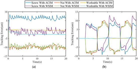
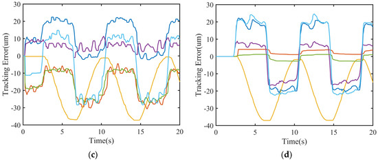
Figure 17.
Tracking error of screw, nut and worktable with ACIM or WSIM under different base speeds and driving modes: (a) two-axis same-speed driving mode with the base speed of 6 mm/s; (b) two-axis same-speed driving mode with the base speed of 0 mm/s; (c) two-axis different-speed driving mode with the base speed of 6 mm/s; (d) two-axis different-speed driving mode with the base speed of 0 mm/s.
Table 7.
Tracking error with ACIM and WSIM for different driving modes.
Compared with the control strategy of feed-forward friction compensation based on the ACIM and PID, the strategy based on the WSIM and PID can avoid the identification error caused by different driving modes. The mean value of the tracking error of the screw, nut and worktable with WSIM is smaller than that with ACIM in the different-speed driving mode, no matter if it is 6 mm/s or 0.
But that is not the same-speed mode case, where the error of the worktable with the WSIM is greater than that with the ACIM. That is because of the specialty of the structure of the TDMS, as illustrated in Section 5.3, with a quasi-static worktable and base speed of zero, which will be further studied for this research. Because the research object of the WSIM is the whole system, it is impossible to ensure the error stability of worktable, with no power, when the randomness of the same-speed driving mode exists. Therefore, the standard deviation of the worktable with the WSIM at the same speed is greater than that of the ACIM. The ACIM can ensure the stability and quasi-stop accuracy of the workbench in the quasi-stationary state, so the ACIM compensation for the synchronous acceleration stage and the WSIM compensation for the differential stage can be adopted to further improve the accuracy.
The velocity of the screw, nut and worktable with the ACIM and WSIM is shown in Figure 18. From Figure 18a, the speed of the workbench of the WSIM is closer to the command value, and the speed change of the screw and nut motors is smoother than that of the ACIM. From Figure 18b, we can see that during the transition phase the screw and nut motors under the WSIM change more gently from the static state. The reason for these phenomena is that the friction model of the system under the ACIM integrates the friction model of each component, and the parameters of the friction model of each component have different trends. However, the friction model of the system under the WSIM is obtained according to the friction model of the whole system in different operating states, so it has a natural smoothness.
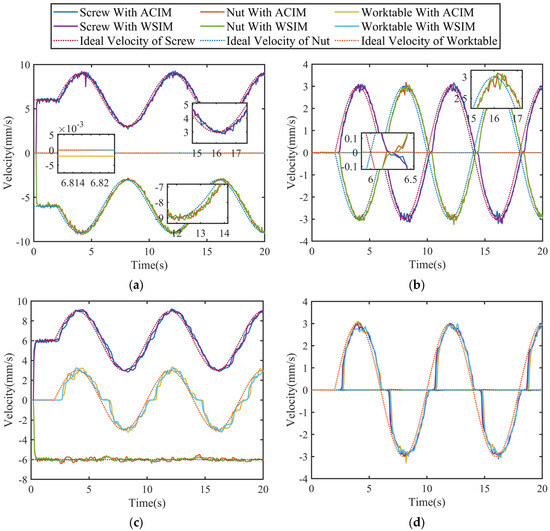
Figure 18.
Velocity–time curve of screw, nut and worktable with ACIM or WSIM under different base speeds and driving modes: (a) two-axis same-speed driving mode with the base speed of 6 mm/s; (b) two-axis same-speed driving mode with the base speed of 0 mm/s; (c) two-axis different-speed driving mode with the base speed of 6 mm/s; (d) two-axis different-speed driving mode with the base speed of 0 mm/s.
From Figure 18c,d, the curves under the WSIM during the transition phase between hysteresis and sliding always accelerate faster than the curves under the ACIM. Thus, the WSIM has a higher compensation accuracy than the ACIM in the hysteresis phase.
5.4.2. LuGre or GMS Friction Model
Let the two motors run at dual drive at same and different speeds with the velocity of transformation along the sine curve. In order to observe the effect of different friction models on the performance of the bench, full closed-loop error compensation and feed-forward friction compensation with LuGre and the Maxwell model is conducted.
The tracking error of the screw, nut and worktable is shown in Figure 19. And the mean value and standard deviation of error is shown in Table 8. The mean error of the screw, nut and worktable with the GMS friction model is smaller than that with the LuGre friction model. The standard deviation of the workbench with the GMS friction model is smaller than that with the LuGre model. Therefore, the TDMS with the GMS friction model has better accuracy and stability than that with the LuGre friction model. It is because the GMS has more variable parameters (Stribeck factor and lag parameter ).
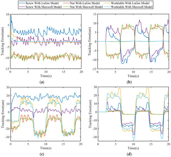
Figure 19.
Tracking error of screw, nut and worktable with LuGre or GMS under different base speeds and driving modes: (a) two-axis same-speed driving mode with the base speed of 6 mm/s; (b) two-axis same-speed driving mode with the base speed of 0 mm/s; (c) two-axis different-speed driving mode with the base speed of 6 mm/s; (d) two-axis different-speed driving mode with the base speed of 0 mm/s.
Table 8.
Tracking error with LuGre and GMS for different driving modes.
The velocity of the screw, nut and worktable with the LuGre and GMS is shown in Figure 20. From Figure 20a, the speed of the workbench of the GMS is closer to the command value, and the speed change of the screw and nut motors is smoother than that of the LuGre. From Figure 20b, we can see that during the transition phase the screw and nut motors under the LuGre change more gently from the static state. The reason for these phenomena is that the GMS friction model uses multiple linear friction units to describe the hysteresis phase, while the LuGre model is described using a first-order differential equation.
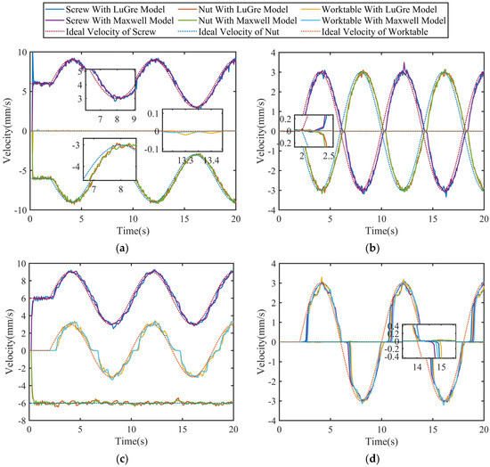
Figure 20.
Velocity–time curve of screw, nut and worktable with LuGre or GMS under different base speeds and driving modes: (a) two-axis same-speed driving mode with the base speed of 6 mm/s; (b) two-axis same-speed driving mode with the base speed of 0 mm/s; (c) two-axis different-speed driving mode with the base speed of 6 mm/s; (d) two-axis different-speed driving mode with the base speed of 0 mm/s.
From Figure 20c,d, the curves under the GMS during the transition phase between hysteresis and sliding always accelerate faster than the curves under the LuGre. Thus, GMS has a higher compensation accuracy than LuGre in the hysteresis phase.
6. Conclusions
In this study, a two-axis differential micro-feed system’s (TDMS) friction is modeled using the generalized Maxwell sliding (GMS) friction model. By comparing the hysteresis curves of LuGre and GMS friction models in a two-axis differential-speed mode, the performance difference between the two models in describing the nonlocal memory phenomenon is analyzed. The GMS model can better describe the nonlocal memory phenomenon of the TDMS better than the LuGre model and has a higher friction prediction accuracy (16.7% in co-speed mode, 26% in differential-speed mode) and stability (59.8% in co-speed mode, 4.68% in differential-speed mode) for it.
In order to address the variations in the identification results under various operating situations brought on by the properties of the TDMS, a novel full-system friction model parameter identification method (WSIM) is developed. Additionally, the two-axis co-speed and two-axis differential-speed parameters of the TDMS’s dynamic and static friction models are identified using the WSIM. The system is made to operate at sinusoidal varying speeds with different references in the two-axis differential-speed and two-axis co-speed modes. The results of the all-components friction model parameter identification method (ACIM) proposed by Feng and the feed-forward friction compensation under the WSIM proposed in this paper are compared and analyzed. In the two-axis co-speed start-up phase (table stationary), the ACIM has a higher recognition accuracy (86.9%) and better operating stability (80.8%) than the WSIM. In the two-axis differential-speed phase (table running), the WSIM has a higher recognition accuracy (58.0%) and stability (55.1%) than the ACIM. Therefore, a combination of the ACIM and WSIM can be used for feed-forward friction compensation to improve control accuracy and stability.
The effects of different base speeds on the parameters of the static friction model in differential-speed mode were observed, and the reasons for the special changes in the Stribeck curves were explained by dynamics analysis. With this, the Stribeck curve of the nut in the TDMS when the screw is used as the drive axis is corrected.
In conclusion, the feed-forward friction compensation results of applying the GMS friction model in this paper are better than the LuGre friction model, which has high accuracy and stability in the static friction phase and better accuracy in describing the nonlocal memory phenomenon in the dynamic friction phase. And the novel WSIM has higher recognition accuracy and operating stability than the ACIM when the worktable runs. In order to obtain a better performance, the system can be compensated by the WSIM when the worktable runs and the ACIM when the system starts. This is of great significance for the precise servo control and smooth feeding of 2-DOF driven machines.
However, the technical difficulties and pending problems of two-axis co-speed starting are derived. Moreover, the nonlinear characteristics, like the drift and backlash when the two axes start at the same speed, may not perform so well. The steady starting of the system can be researched in the future. In addition, the lubrication system of the experimental equipment in this article is not systematic enough; it will be equipped with a better lubrication system and vibration isolation equipment to achieve higher experimental precision.
Author Contributions
Conceptualization, Z.Z. and X.F.; methodology, Z.Z and X.F.; software, Z.Z. and P.L.; validation, Z.Z.; formal analysis, Z.Z. and X.F.; investigation, Z.S.; resources, X.F., P.L. and A.W.; data curation, Z.Z. and A.W.; writing—original draft preparation, Z.Z.; writing—review and editing, Z.Z., X.F., P.L., A.W. and Z.S.; visualization, Z.Z. and A.W.; supervision, X.F.; project administration, X.F.; funding acquisition, X.F. All authors have read and agreed to the published version of the manuscript.
Funding
This work was supported by the Key Research and Development Plan of Shandong Province (2022CXGC010101) and the National Natural Science Foundation of China (No. 51875325).
Conflicts of Interest
The authors declare no conflict of interest. The funders had no role in the design of the study; in the collection, analyses, or interpretation of data; in the writing of the manuscript; or in the decision to publish the results.
References
- Gao, X.; Li, Z.; Wu, J.; Xin, X.; Shen, X.; Yuan, X.; Yang, J.; Chu, Z.; Dong, S. A Piezoelectric and Electromagnetic Dual Mechanism Multimodal Linear Actuator for Generating Macro- and Nanomotion. Research 2019, 2019, 8232097. [Google Scholar] [CrossRef] [PubMed]
- Iqbal, S.; Malik, A. A review on MEMS based micro displacement amplification mechanisms. Sens. Actuators A Phys. 2019, 300, 111666. [Google Scholar] [CrossRef]
- Tian, W.; Wang, H. Static analysis of a large-displacement low-voltage micro actuator. In Proceedings of the 2011 International Symposium on Advanced Packaging Materials (APM 2011), Xiamen, China, 25–28 October 2011; pp. 163–167. [Google Scholar]
- Du, F.; Li, P.; Wang, Z.; Yue, M.; Feng, X. Modeling, identification and analysis of a novel two-axis differential micro-feed system. Precis. Eng. 2017, 50, 320–327. [Google Scholar] [CrossRef]
- Wang, Z.; Feng, X.; Du, F.; Li, H.; Su, Z. A novel method for smooth low-speed operation of linear feed systems. Precis. Eng. 2019, 60, 215–221. [Google Scholar] [CrossRef]
- Wang, Z.; Feng, X.; Li, P.; Du, F. Dynamic modeling and analysis of the nut-direct drive system. Adv. Mech. Eng. 2018, 10, 1687814018810656. [Google Scholar] [CrossRef]
- Yu, H.; Feng, X. Modelling and analysis of dual driven feed system with friction. J. Balk. Tribol. Assoc. 2015, 21, 736–752. [Google Scholar]
- Liu, A. Analysis of Friction Characteristics and Research on Compensation Method for Low Speed Servo System; Harbin Institute of Technology: Heilongjiang, China, 2021. [Google Scholar]
- Tjahjowidodo, T.; Al-Bender, F.; Van Brussel, H.; Symens, W. Friction characterization and compensation in electro-mechanical systems. J. Sound Vib. 2007, 308, 632–646. [Google Scholar] [CrossRef]
- Rong, W.B.; Liang, S.; Wang, L.F.; Zhang, S.Z.; Zhang, W. Model and Control of a Compact Long-Travel Accurate-Manipulation Platform. IEEE/ASME Trans. Mechatron. 2017, 22, 402–411. [Google Scholar] [CrossRef]
- Schneider, F.; Das, J.; Kirsch, B.; Linke, B.; Aurich, J.C. Sustainability in Ultra Precision and Micro Machining: A Review. Int. J. Precis. Eng. Manuf.-Green Technol. 2019, 6, 601–610. [Google Scholar] [CrossRef]
- Huang, S.N.; Liang, W.Y.; Tan, K.K. Intelligent Friction Compensation: A Review. IEEE/ASME Trans. Mechatron. 2019, 24, 1763–1774. [Google Scholar] [CrossRef]
- Delibas, B.; Koc, B. A Method to Realize Low Velocity Movability and Eliminate Friction Induced Noise in Piezoelectric Ultrasonic Motors. IEEE/ASME Trans. Mechatron. 2020, 25, 2677–2687. [Google Scholar] [CrossRef]
- Li, F.T.; Ma, L.; Mi, L.T.; Zeng, Y.X.; Jin, N.B.; Gao, Y.L. Friction identification and compensation design for precision positioning. Adv. Manuf. 2017, 5, 120–129. [Google Scholar] [CrossRef]
- Piasek, J.; Patelski, R.; Pazderski, D.; Kozłowski, K. Identification of a Dynamic Friction Model and Its Application in a Precise Tracking Control. Acta Polytech. Hung. 2019, 16, 83–99. [Google Scholar] [CrossRef]
- Ge, Z.; Zhu, H. Complicate Tribological Systems and Quantitative Study Methods of Their Problems. Tribology 2002, 22, 405–408. [Google Scholar]
- Yu, H.; Feng, X.; Sun, Q. Kinematic analysis and simulation of a new type of differential micro-feed mechanism with friction. Sci. Prog. 2020, 103, 36850419875667. [Google Scholar] [CrossRef] [PubMed]
- Du, F. Modeling and Analysis for a Novel Dual-axis Differential Micro-feed System. J. Mech. Eng. 2018, 54, 195–204. [Google Scholar] [CrossRef]
- Swevers, J.; Al-Bender, F.; Ganseman, C.G.; Prajogo, T. An integrated friction model structure with improved presliding behavior for accurate friction compensation. IEEE Trans. Autom. Control. 2000, 45, 675–686. [Google Scholar] [CrossRef]
- Lampaert, V.; Al-Bender, F.; Swevers, J. A generalized Maxwell-slip friction model appropriate for control purposes. In Proceedings of the 2003 IEEE International Workshop on Workload Characterization (IEEE Cat. No. 03EX775), St. Petersburg, Russia, 20–22 August 2003; IEEE: Piscataway, NJ, USA, 2003; pp. 1170–1177. [Google Scholar]
- Al-Bender, F.; Lampaert, V.; Swevers, J. The generalized Maxwell-slip model: A novel model for friction Simulation and compensation. IEEE Trans. Autom. Control. 2005, 50, 1883–1887. [Google Scholar] [CrossRef]
- Zschäck, S.; Büchner, S.; Amthor, A.; Ament, C. Maxwell Slip based adaptive friction compensation in high precision applications. In Proceedings of the IECON 2012-38th Annual Conference on IEEE Industrial Electronics Society, Montreal, QC, Canada, 25–28 October 2012; IEEE: Piscataway, NJ, USA, 2012; pp. 2331–2336. [Google Scholar]
- Farhat, N.; Mata, V.; Page, A.; Valero, F. Identification of dynamic parameters of a 3-DOF RPS parallel manipulator. Mech. Mach. Theory 2008, 43, 1–17. [Google Scholar] [CrossRef]
- Yang, H.; Zhao, Y.; Li, M.; Zhou, Y.J. Study on the friction torque test and identification algorithm for gimbal axis of an inertial stabilized platform. Proc. Inst. Mech. Eng. Part G-J. Aerosp. Eng. 2016, 230, 1990–1999. [Google Scholar] [CrossRef]
- Du, F. Research on Friction Modeling Analysis and Compensation of Two-Axis Differential Micro-Feed Servo System; Shandong University: Jinan, China, 2018. [Google Scholar]
- Lu, Z.; Feng, X.; Su, Z.; Liu, Y.; Yao, M. Friction Parameters Dynamic Change and Compensation for a Novel Dual-Drive Micro-Feeding System. Actuators 2022, 11, 236. [Google Scholar] [CrossRef]
- Chauhan, D.; Singhvi, N. Prediction of effective thermal conductivity of nanofluids by modifying renovated Maxwell model. J. Thermoplast. Compos. Mater. 2016, 30, 289–301. [Google Scholar] [CrossRef]
- Ruderman, M.; Hoffmann, F.; Bertram, T. Modeling and Identification of Elastic Robot Joints with Hysteresis and Backlash. IEEE Trans. Ind. Electron. 2009, 56, 3840–3847. [Google Scholar] [CrossRef]
- Marques, F.; Flores, P.; Claro, J.C.P.; Lankarani, H.M. Modeling and analysis of friction including rolling effects in multibody dynamics: A review. Multibody Syst. Dyn. 2018, 45, 223–244. [Google Scholar] [CrossRef]
- Rizos, D.D.; Fassois, S.D. Presliding friction identification based upon the Maxwell Slip model structure. Chaos 2004, 14, 431–445. [Google Scholar] [CrossRef] [PubMed]
Disclaimer/Publisher’s Note: The statements, opinions and data contained in all publications are solely those of the individual author(s) and contributor(s) and not of MDPI and/or the editor(s). MDPI and/or the editor(s) disclaim responsibility for any injury to people or property resulting from any ideas, methods, instructions or products referred to in the content. |
© 2023 by the authors. Licensee MDPI, Basel, Switzerland. This article is an open access article distributed under the terms and conditions of the Creative Commons Attribution (CC BY) license (https://creativecommons.org/licenses/by/4.0/).