A Global Trajectory Planning Framework Based on Minimizing the Risk Index

Abstract

At present, autonomous mobile robots are widely used in industrial and commercial fields. However, although the global path searched by existing mobile robot path planning methods has no collision with obstacles, there is a problem in that the path is close to obstacles and is not smooth, and there is a collision safety risk when the robot is actually moving. To solve the above problems, this paper proposes a global path planning method based on minimizing the risk index. Firstly, the distance calculation method of the heuristic function of the traditional graph search algorithm is improved to reduce the number of nodes in the search space. Additionally, by selecting the appropriate search neighborhood, the search efficiency and path smoothness of the algorithm are improved. Thirdly, to increase the distance between the original search path and obstacles, the risk index path search strategy is proposed. Finally, the minimized snap trajectory smoothing method with a safe corridor is used to smooth the original waypoint. Both simulation and real robot experimental results show that the minimum distance between waypoints and obstacles is increased by 43.72% on average, and the number of trajectory inflection points are reduced by 75.12% on average after optimization. As such, the proposed method can fully guarantee safety and generate smooth mobile robot paths in global trajectory planning tasks.

1. Introduction

In recent years, mobile robots have had the advantages of flexible application, safety, and high efficiency in production and transportation, and account for an increasing proportion of the factors improving social productivity. Mobile robots have a huge demand in both industrial and commercial scenes, and have broad application prospects [1]. For mobile robots, they need to move autonomously in different environments and complete various tasks. Therefore, safe navigation is very important for robots, and path planning is an important aspect in determining whether navigation is safe or not. Safe and autonomous movement of the mobile robot is a prerequisite for robot task completion. Motion planning mainly consists of front-end path planning and back-end trajectory optimization. Path planning technology is a very important and basic technology in the practical application of mobile robots [2].

At present, there are many path planning algorithms, among which the graph search algorithm is widely adopted [3]. Although the global path planning based on a graph search algorithm can search for the global optimal solution, the generated path is usually not suitable as a direct executable path input of the trajectory tracking control module. The main reason is that the current path search algorithm usually treats the robot as a particle and expands the grid map, and the expansion distance is usually the radius of the robot. Although the path obtained by this graph search method does not collide with obstacles theoretically, the waypoint is close to obstacles.

If the mobile robot travels according to this path, there will be positioning and control errors in the process of robot navigation, so there is a safety risk of collision with obstacles in the process of robot navigation. As shown by the arrow in Figure 1, if the waypoint is too far away from the obstacle, the path length will increase, and if the distance is too close, the safety risk of collision will increase. In view of the above problems, the research focus of this paper is how to ensure that a followable global path with the lowest security risk is sought and obtained for the robot. The original path obtained by searching in the original graph is a series of discrete waypoints. If the waypoints are simply connected, there will be uneven broken lines. If path-tracking control is carried out directly, the robot will move unevenly. Therefore, it is necessary to smooth the trajectory of the original waypoint.

In order to solve the above problems, this paper proposes a global path planning algorithm based on minimizing the risk index (CRI-A*), which can plan a path away from obstacles and with a minimum risk index according to the environmental grid map. In the graph search algorithm, only the value of a heuristic function is considered; the cost map value of the current grid and the danger index of the waypoint are also added. At the same time, the minimized snap path optimization method with a safe corridor is used to smooth the trajectory of the original waypoint. Finally, a safe and smooth driving track is obtained. The global path planning algorithm is suitable for commercial and industrial application scenarios, as it makes path planning more efficient and concurrently improves the use safety and security of mobile robots in various complex scenarios.

The content of this paper is organized as follows: Section 2 introduces the research status of the global path planning algorithm in improving path security and trajectory smoothing. Section 3 introduces the global path planning algorithm and trajectory smoothing method based on minimizing the risk index; In Section 4, the ROS simulation and real-scene global path planning experiments are carried out to verify the proposed method. The experimental results show the effectiveness and robustness of the proposed method. In Section 5, the conclusions of this paper are presented, and future research work is proposed according to the shortcomings of the method.

2. Related Work

From the research status of global path planning for mobile robots, searching for an accessible path with high safety factors is one of the research hotspots of many scholars. To avoid the conflict between the planned path and obstacles, the robot needs to plan the global optimal driving path from the starting point to the target point in advance. To solve the path planning problem of mobile robots, many algorithms have been proposed, including the probabilistic roadmap (PRM) [4,5], fast extended random tree (RRT) [6,7], artificial potential field (APF) [8], genetic algorithm (GA) [9], ant colony algorithm (ACO) [10], dynamic window method [11], etc.

The convergence speed of the ant colony algorithm is slow and easily falls into the local optimal state. The search efficiency of the RRT algorithm is high, but the obtained path is often far from the global optimal path. Although the artificial potential field algorithm has a simple structure and is easy to implement, it has problems such as unattainability of some goal positions. Compared with these algorithms, the A* algorithm has the advantages of a simple principle, easy implementation, and good robustness [12], so it has been widely studied and applied in the field of global path planning. However, the algorithm still has some shortcomings; for example, the impact of the distance between the path planned by the robot and the obstacle on the safety of the robot has not been fully considered.

The path planned by the traditional A* algorithm is often close to obstacles. In actual implementations, there will be the danger of collision between robots and obstacles [13]. To avoid collision between robots and obstacles, the most common method is to expand obstacles at a fixed distance in a grid-based path planning algorithm, but a simple multilayer expansion of obstacles will lead to an increase in obstacle area and an increase in planned path length [14]. Zhang et al. [15] proposed to define the security threat cost of a node according to the minimum distance between the node and obstacles, and introduced it into the cost function of the A* algorithm to improve the security of the planned path. Zhan et al. [16] added parameters such as route height and radar detection probability to the evaluation function, so that the planned route could be as far away from the dangerous area as possible. Park et al. [17] used obstacle distance and dangerous point parameters to build a safe space to deal with potential risks, and introduced risk cost into the heuristic function of the algorithm to ensure that there was enough safe distance between the path and obstacles. Bayili et al. [18] proposed an improved A* algorithm with limited damage, which considers the dangerous areas in the map, takes the minimum damage as the feasibility criterion, and considers the collision risk to obtain a safer path. Chen et al. [19] introduced the best neighborhood matrix to search for obstacles, and improved the heuristic function combined with partition adaptive distance information, which improved the path security, but led to a sharp increase in the search direction of the safe distance matrix, which seriously reduced the search efficiency. Wang et al. [20] added the safe distance matrix to the standard A* algorithm and improved its heuristic function to ensure the security of path search. Sun et al. [21] proposed a fuzzy path planning algorithm, which ensures the safety of the planned path by imposing angular velocity constraints on the robot. However, the above method only ensures the safety of waypoints, and cannot guarantee the safety of trajectories generated according to waypoints. The method based on the risk index has been widely used on unmanned aerial vehicles [22], underwater vehicles [23], and ground mobile robots [24], but they still have some safety hazards.

After obtaining a safe waypoint, it is necessary to connect the waypoint to a smooth path. Path smoothing of mobile robots must meet certain constraints, such as continuity and security. Continuity mainly refers to geometric tangential continuity or curvature continuity. Safety requires that the planned road be far enough away from obstacles. At present, the commonly used path smoothing methods are mainly divided into using special curve smoothing methods and interpolation-based methods. The special curve smoothing method takes the route points obtained by the path search method as the known input and then uses the special mathematical curve to generate a feasible smooth path. Commonly used curves include Durbin’s curve [25], the cyclotron curve [26], and so on. Using the above-mentioned special curve method directly to smooth the path usually requires changing the original path, which can not guarantee that the collision-free path is generated. Therefore, the algorithm needs an extra processing step to check whether the optimized path still does not collide with obstacles, which is very time-consuming and affects the solution speed.

Path optimization methods based on interpolation mainly include polynomial interpolation [27], Bezier curve interpolation [28], and spline curve interpolation [29]. Generally speaking, path smoothing based on interpolation is easy to calculate, and the curves can be connected to obtain the required shape, and the safe area can also be limited. However, when there are too many interpolation curve coefficients, trajectory optimization takes a long time, which is not suitable for online applications. In interpolation problems, spline interpolation is generally superior to polynomial interpolation. Even if spline curves use low-order polynomials, the results produced by them are still similar, which effectively prevents the Runge phenomenon when using high-order polynomials. Therefore, this paper combines the reasonable use of special curves and through the safe search of the waypoint to ensure the safety of the path and the smoothness of the trajectory.

The main contributions of this paper are multifaceted. A framework for safe trajectory generation of mobile robots is proposed. In the front-end path search, a global path planning method based on the minimized hazard index is proposed. In back-end trajectory optimization, a minimized snap function is used for trajectory smoothing. Firstly, this paper uses an improved distance calculation method, which can reduce the number of search nodes in the graph search algorithm. Secondly, the results of the 4-neighborhood, 8-neighborhood, and 24-neighborhood searches are compared, and the optimal search neighborhood is selected as the search neighborhood of this path planning method. Secondly, aiming at the problem of the route point being too close to the obstacle in path planning, a global path planning method based on minimizing the danger index is proposed. Finally, the minimized snap with a security corridor constraint is used to generate trajectory. In the experiment, the global path planning method proposed in this paper can ensure the security and smoothness of the mobile robot path.

3. Methodology

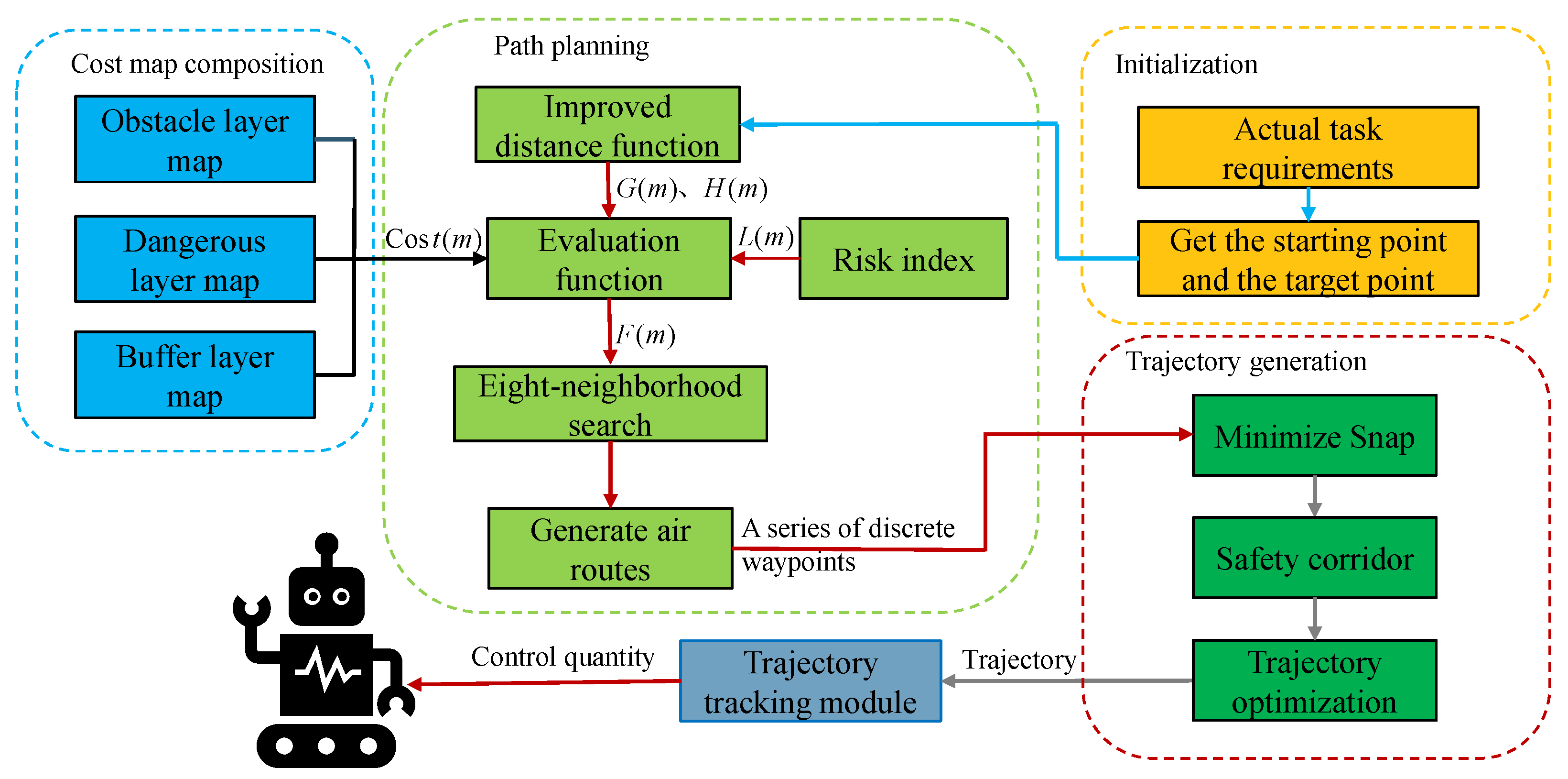
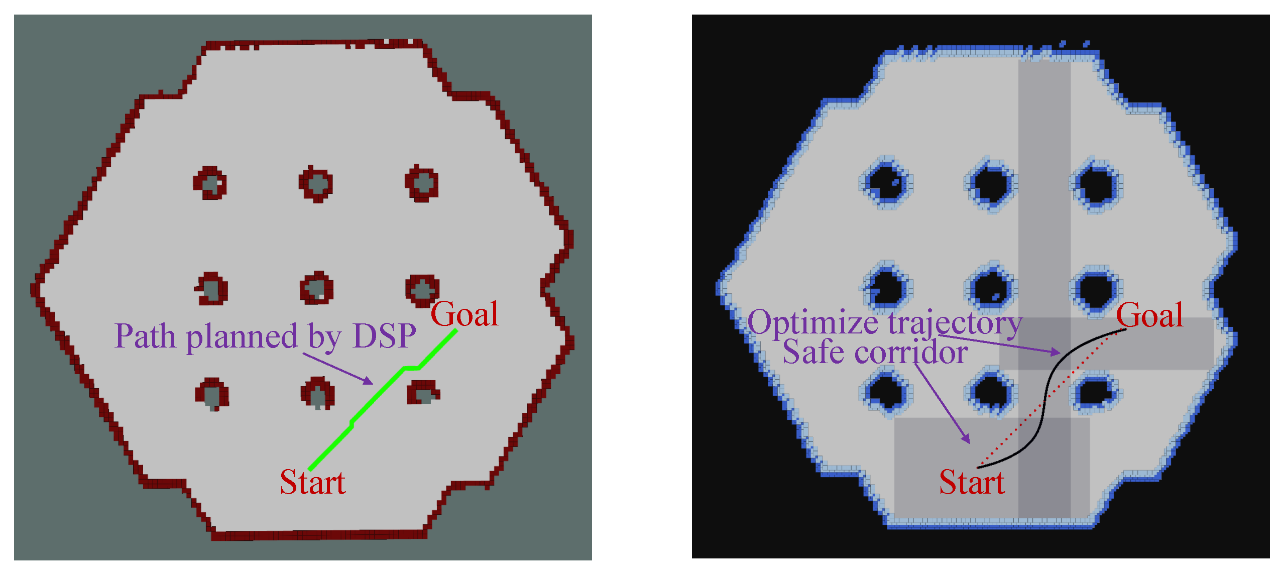
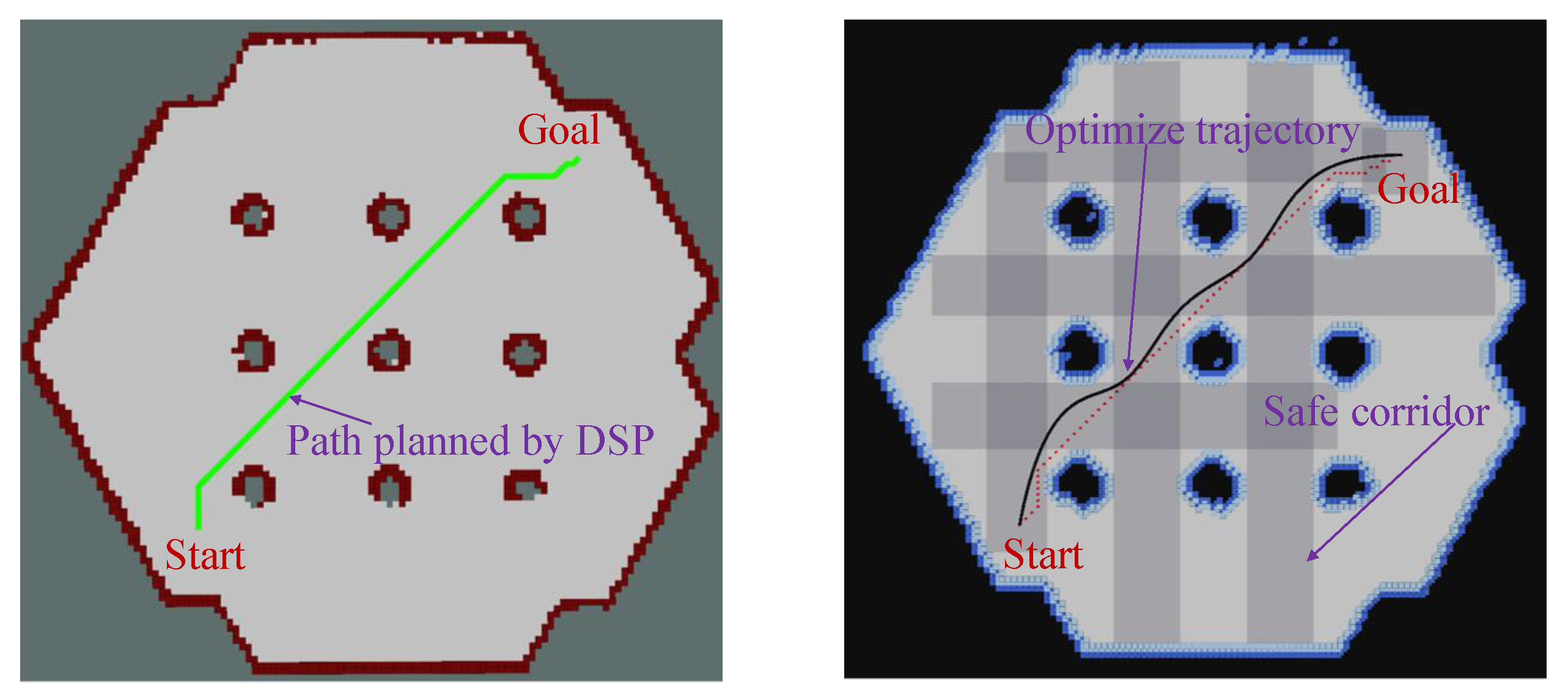
Firstly, this paper introduces the overall structure block diagram, elaborates on the graph search algorithm that is widely used in path planning, and analyzes its principle and the composition of the evaluation function in detail. Secondly, the distance calculation method in the heuristic function of the graph search algorithm is described. Aiming at the traditional Euclidean distance calculation method, an improved distance calculation method, which effectively reduces the number of search nodes of the algorithm, is proposed. Then, the path planning results of different search neighborhoods are compared and the appropriate search neighborhoods are selected. Finally, this paper introduces the robot safe motion planning method based on minimized hazard index and uses minimized Snap method with the safe corridor to generate trajectory. Experiments are carried out in ROS simulation environments and real scenes. The experimental results show that compared with traditional path planning algorithms, the proposed algorithm in this paper has more advantages in global path security and smoothness.

3.1. Overall Block Diagram of Algorithm

The whole structure diagram of the algorithm is shown in Figure 2. First, the environment information is converted into a grid map and the grid map information is transmitted to the cost map module. According to the information on the obstacle layer, the danger layer and buffer layer are obtained, which are added to the evaluation function of the CRI-A* algorithm as the substitute value of each grid. At the same time, the distance calculation function can reduce the number of search nodes by using the improved distance calculation method proposed in this paper. To further control the distance between the planned path and obstacles, a danger index is introduced. When the planned path is farther away for obstacles, the danger index value reduces. This algorithm uses eight-neighborhood searches, and finally obtains the path that meets the security requirements at the same time. The path points are passed as input to the trajectory generation module, and the optimized trajectory is obtained by minimizing the snap function and imposing security corridor constraints. Finally, the optimized trajectory is passed to the trajectory tracking module for robot trajectory tracking.

3.2. Overview of Graph Search Algorithm

The graph search algorithm can obtain the shortest path and reduce the number of search nodes at the same time based on the heuristic function. This method uses known information or experience to search to find a solution to the problem, and the search process intelligently avoids searching in unfavorable areas in the search space, thus speeding up the search process. The heuristic function of the graph search algorithm combines the Dijkstra algorithm with the heuristic function of best-first search. The extension points in the search process of the algorithm are stored in the open list, while the environment nodes of obstacles are stored in the closed list. The algorithm starts from the starting point, calculates the value of each node by using a heuristic function, and selects the node with the lowest value to expand until the target node is searched, and thus obtains the path with the lowest value, that is, the optimal path. Figure 3 is an example diagram of the meaning of each part of the evaluation function of the A* algorithm. The evaluation function of the algorithm is given in Equation (1).

$$F\left(m\right)=G\left(m\right)+H\left(m\right)$$

(1)

where m represents the extended node, $F\left(m\right)$ is the heuristic estimation function from the starting node through node m to the target node, $G\left(m\right)$ is the actual generation value from the starting point to the current node m, and $H\left(m\right)$ is the heuristic generation value of the current node m to the end point.

3.3. Construction of Grid Map Based on Risk Factor Grade

At present, grid map is widely used to represent environment information in robot path planning. Grid map is composed of a series of pixels, which correspond to a certain gray value within 0–255. The gray value of obstacle area is 0, and the gray value of blank grid is 255. Therefore, it is necessary to transform the environment information of robot into grid information. Blank grid is a space where robots can pass freely, while black grid represents the position of obstacles. Whether the obstacles can completely occupy the grid or not, the grid should be marked as an obstacle area. Robots cannot pass through the black grid, and robots need to plan a collision-free route from the space where the blank grid is located.

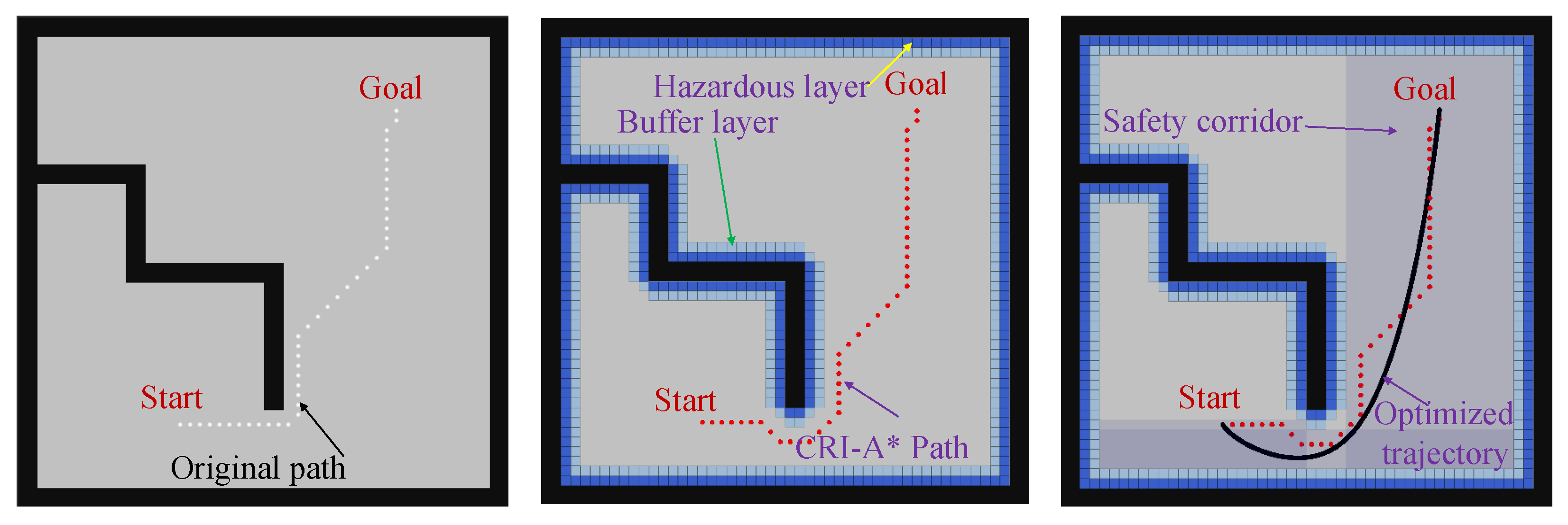
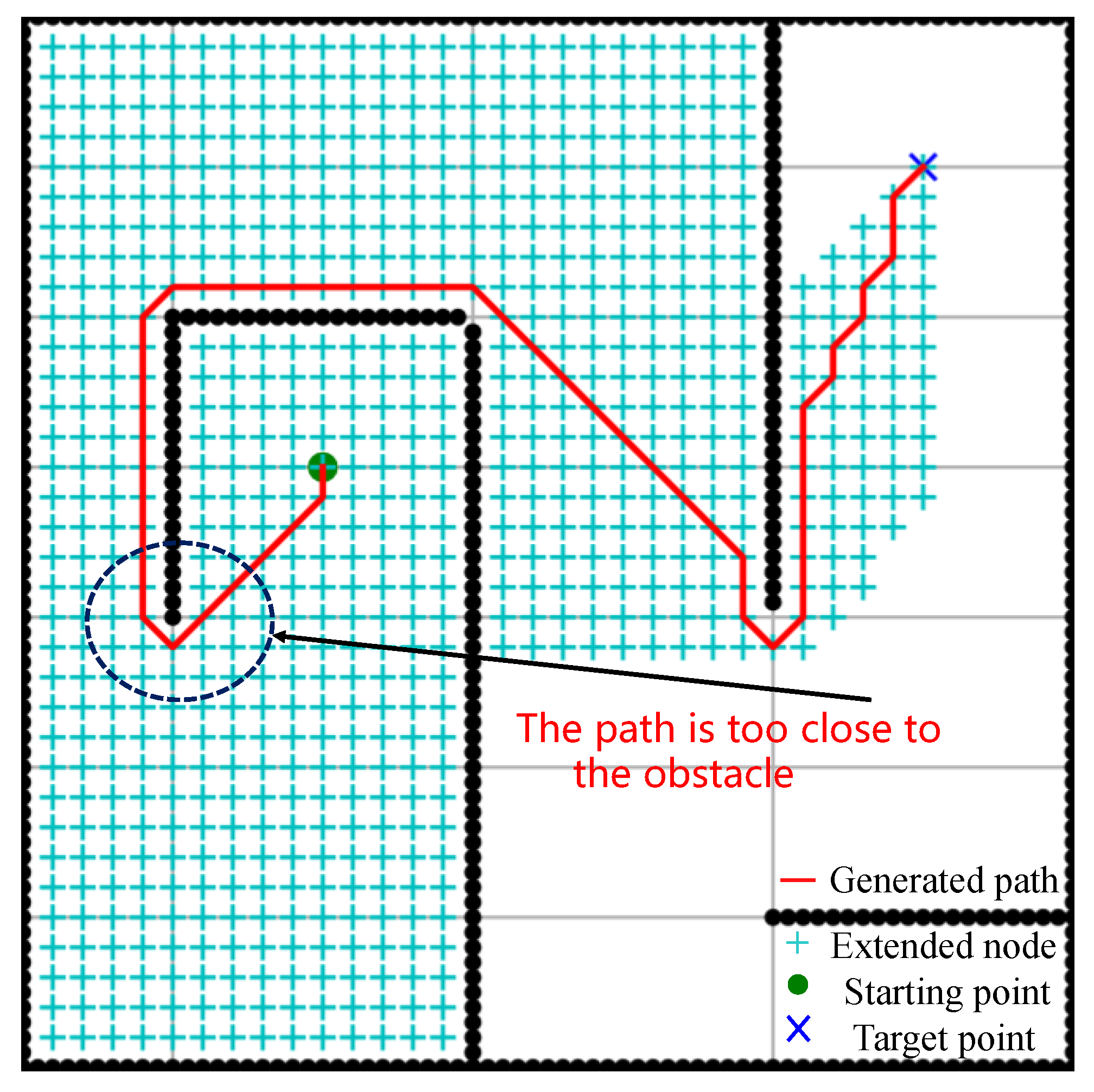
To ensure the distance between the planned path and obstacles, the cost map [30] is introduced into the algorithm. The cost map in this paper is mainly composed of three layers, which are the obstacle layer, danger layer, and buffer layer. The specific cost map is shown in Figure 4. When the raster map is loaded as a cost map, the cost map needs to be expanded according to the size of obstacles, but there are no obstacles in the expansion area, so it is necessary to use substitute value to express the cost of collision between robot and obstacles within the expansion distance of obstacles. Specifically, the obstacle layer is constructed according to the environmental information of the robot, which is represented in black in the figure and is the bottom layer of the whole cost map, in which the danger level of obstacles should be the highest, and the planned path should not collide with or cross it. The dangerous layer is indicated in dark blue on the map, which mainly expands the obstacles in the cost map. In practical application, the expansion distance can be set as the radius r of the tangent circle of the robot, and the path planned by the robot should intersect with the dangerous area as little as possible. The buffer layer is further expanded based on the dangerous area, which is represented by light blue in the figure. In practical applications, the r-2r area can be set as the buffer layer, and the robot will not collide with obstacles in this area. However, to prevent the occurrence of uncontrollable factors and leave enough safety margin, the robot should try to avoid entering the buffer layer when the space allows. The cost map is obtained by superimposing the obstacle layer, danger layer, and buffer layer.

To correctly express the generation value of different positions in the map, the distance between the current node and the obstacle is considered and converted into the gray value of the point. The conversion formula is given as Equation (2).

$$G_{\mathrm{v}}=\left\{\begin{array}{cc}254\hfill & d<r\hfill \\ 253e^{-\omega (d-r)}\hfill & r\le d\le 2r\hfill \\ 0\hfill & 2r<d\hfill \end{array}\right.$$

(2)

where d is the distance between the robot and the obstacle, $\omega$ is the weight coefficient with the value of 0.5, $G_{\mathrm{v}}$ is the gray value of the point, and the gray value of the grid is converted into the substitute value of 0 ∼ 100 in the cost map. The substitute value cost calculation formula of the points is given in Equations (3) and (4).

$$Cost\left(m\right)=\left\{\begin{array}{cc}99(q-FG)/(OG-FG)& ,FG<q<OG\\ 100& ,OG<q\\ 0& ,q<FG\end{array}\right.$$

(3)

$$q=\frac{255-x}{255}$$

(4)

where q is the ratio of the gray values of the current grid, OG is the threshold of the occupied grid, x is the image value of the grid, and FG is the threshold of the idle grid. When q is greater than OG, it can be considered as an obstacle grid with a generation value of 100. When q is less than FG, it can be considered as completely idle, with a generation value of 0. When q is between FG and OG, conversion to a value between 0 and 100 is needed. In such cases (between FG and OG), the closer q is to obstacles, the more dangerous it is, and as such, the higher its generation value should be. The schematic diagram of path planning in the cost map is shown in Figure 5. For clear representation, only one layer of grid around obstacles is constructed as a dangerous layer, but no buffer layer is constructed. The algorithm needs to design a path from the starting point to the target point without passing through obstacles, and the planned path should avoid passing through the dangerous layer area as much as possible.

After determining the danger value of each point, if the free space of the environment is large because the map generation value outside the buffer layer is 0, the path planned by the robot is often close to the edge of the obstacle, and a large amount of free space is not used. If a function can be applied so that the planned path can keep a certain safe distance from obstacles, the designed danger index $L\left(m\right)$ can be determined as follows:

$$L\left(m\right)=\frac{1}{\alpha d\left(m\right)+1}$$

(5)

where $\alpha$ is the distance factor given the value 10 and $d\left(m\right)$ is the minimum Euclidean distance between the robot and the obstacle. It can be seen from Equation (5) that when the distance between the path and the obstacle is very small, the danger index value is very large.

3.4. Improvement of Distance Calculation Method

In the path planning of mobile robots, a heuristic function is a function used to estimate the distance between the current node and the target state, which is used to guide the search of the path planning algorithm. This kind of search is called “Heuristic Search”, and its function is to help the algorithm find a high-quality path quickly and avoid invalid search directions as much as possible. The design of the heuristic function needs to consider two factors: accuracy and efficiency. Accuracy refers to whether the heuristic function can reflect the real distance between nodes, and efficiency refers to whether the computational cost of the heuristic function is low. Generally speaking, the more accurate the heuristic function is, the easier it is for the search algorithm to find the optimal path; the simpler the heuristic function, the more time and space the search algorithm saves.

The traditional A* search algorithm is mainly suitable for grid-based environments, and the heuristic function is related to the changing distance between the target point and the current position. The heuristic function is not affected by various obstacles in the robot’s forward path, which makes the algorithm more effective in identifying grids. In the heuristic function of the A* algorithm, the calculation method of distance has a great influence on the number of search nodes of the algorithm. The commonly used distance forms are Euclidean distance, Manhattan distance, and diagonal distance. The following is a brief description of the calculation methods of several distance formulas: the specific expressions of Euclidean distance, diagonal distance, and Manhattan distance between two points in a two-dimensional plane. Equation (6) shows the Euclidean distance calculation method.

$$H\left(m\right)=\sqrt{{(x_{\mathrm{a}}-x_{\mathrm{b}})}^2+{(y_{\mathrm{a}}-y_{\mathrm{b}})}^2}$$

(6)

In Equation (6), a and b represent the position information of the first and last two points, and their coordinates are $(x_{\mathrm{a}},y_{\mathrm{a}})$ and $(x_{\mathrm{b}},y_{\mathrm{b}})$, respectively.

At present, Euclidean distance [31] is the most widely used distance calculation method in path planning. To speed up the algorithm, this paper proposes a new Euclidean distance calculation method, which designs a guide function according to the connection between the starting point and the target point. This method makes the searched nodes as close to the guideline as possible, reduces the number of nodes in the search process, and guides the target point faster. The designed linear guide distance calculation function is given in Equation (7).

$$H\left(m\right)=\frac{\left|a·x_n+b·y_n+c\right|}{\sqrt{\left(a^2+b^2+c^2\right)}}+\sqrt{{(x_{\mathrm{a}}-x_{\mathrm{b}})}^2+{(y_{\mathrm{a}}-y_{\mathrm{b}})}^2}$$

(7)

In Equation (7), the left term represents the degree of deviation between the current node and the line connecting the starting point and target point. The further the current node is away from the line, the greater the value of the equation. a, b, and c are constant coefficients of the first-order function $a·x+b·y+c=0$ formed by the line connecting the starting point and the target point. When the starting point and target point are in a straight line, a and b can be taken as 0, while c cannot be taken as 0.

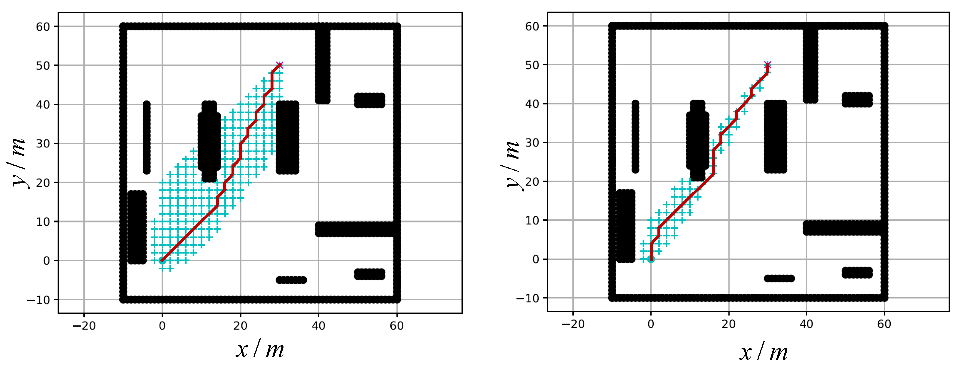
To verify whether the improved distance function can reduce the number of search nodes, simulation experiments are carried out. In a python 3.7 environment, numpy 1.24.2 is used to realize read and write data operations, and matplotlib 3.7.0 functions are also used as a map drawing tool. The path planning algorithm uses traditional Euclidean distance and the improved distance function proposed in this section for simulation and verification in an environment with obstacles. The starting point coordinates are (0, 0), target point coordinates are (32, 50), in Figure 6, a dot represents the starting point, asterisks represent the target point, and “+” marks represent expanded nodes in the search process. Eight is used as the neighborhood search, starting points and target points remain unchanged in the two simulated searches, and the distribution of obstacles also remain unchanged. The results are shown in Figure 6, and related data are shown in

Table 1. Comparison of results of different distance calculation functions.

Heuristic Function	Algorithm Execution Time/s	Number of Turning Points	Total Path Length/m	Number of Search Nodes/Pieces
Euclidean distance	1.79	16	62.58	86
Improved distance	1.37	12	62.42	66

.

By analyzing the experimental results, it can be found that the execution time of the algorithm is shortened by 30.7%, the number of turning points is reduced to 75%, and the number of search nodes is reduced by 23.3%. It can be seen that the new distance calculation method can approach the target point faster with fewer expanding directions, thus effectively reducing the number of search nodes and improving the running efficiency of the algorithm. To better verify the robustness of the distance calculation function, under the same obstacle distribution, different starting points and target points are selected for ten experiments, and the experimental results as shown in the bar chart in Figure 7.

The abscissa in the graph represents the number of experiments, and the ordinate represents the number of search nodes of the A* algorithm. By observing the data in the graph, it can be seen that the number of search nodes obtained using the improved distance function is lower than that of Euclidean distance. The number of search nodes in ten experiments decreases from 15.4% to 30.8%, with an average of 23.5%. It can be found that the improved distance function has an obvious effect on reducing the search nodes of the A* algorithm.

3.5. Determination of Search Neighborhood

In the process of A* algorithm searching for the next node according to the current node, the number of nodes searched every time will determine the execution time of the algorithm and the length of the final path, so it is very important to choose the search neighborhood of the algorithm reasonably [32]. As shown on the left in Figure 8, it is a schematic diagram of the 4-neighborhood search, in which 1 is the position that can be reached by the next search, and 0 is that the current node cannot be searched. That is, in the next node expansion, only nodes in four directions can be searched and put into the open list. In this way, the path angle is usually an integer multiple of π/2, which does not conform to the turning characteristics of the robot. Conversely, the right side in Figure 8 shows a schematic diagram of 8-neighborhood search that is more suitable for robots. In each node expansion, nodes in eight directions outside the node will enter the open list, so that the rotation angle of the path will be further reduced, and each turn angle is an integer multiple of π/4, which will be beneficial to the execution of the robot.

To further improve the minimum moving angle of the robot at each tracking stage, a more accurate angle can be obtained by expanding the unfolding area, which expands the nodes into two layers outside the node to achieve 24-neighborhood search, as shown in Figure 9. With the decrease in the minimum rotation angle, the final planned path length will decrease; however, too large an unfolding range will lead to an increase in the number of nodes searched every time, increasing computational complexity and causing poor real-time performance of the algorithm. To better choose the search neighborhood and weigh the relationship between path length and search time, simulation software is used for analysis.

To better select a search neighborhood, the path planning simulation experiment is carried out in a python 3.7 environment. The simulation environment is a square grid map with a size of 70 m × 70 m. During the experiment, the starting point and target point are kept unchanged, the starting point coordinates are (0, 0), and the target point coordinates are (34, 50). The A* algorithm uses 4 neighborhoods, 8 neighborhoods, and 24 neighborhoods to plan the path, as shown in Figure 10, where the green dot is the starting point, the + sign represents the target point, and the black area is an obstacle.The relevant experimental data are shown in

Table 2. Comparison of results of different search neighborhoods.

Search Neighborhood Number	Algorithm Execution Time/s	Number of Turning Points	Total Path Length/m
4-Neighborhood	1.47	24	82
8-Neighborhood	1.83	10	64.08
24-Neighborhood	2.65	6	58.54

.

By analyzing the experimental results, we can find that the path length of the 4-neighborhood is 27.9% longer than the 8-neighborhood, and the 8-neighborhood is 40.1% longer than the 24-neighborhood. The turning point of the 4-neighborhood is longer than that of the 8-neighborhood, and the 8-neighborhood longer than 24-neighborhood, by 140% and 300%, respectively. The running time of the 4-neighborhood is 19.7% less than the 8-neighborhood, and the 8-neighborhood is less than 24-neighborhood by 44.5%. It can be concluded that with the increase in the number of neighbors, the path length and turning point decreases greatly, but the running speed of the algorithm is sacrificed. To better control the path length and the number of turning points while taking into account the running time of the algorithm, 8 neighbors should be selected as the search neighborhood.

3.6. CRI-A* Algorithm

After the research and analysis of the above two sections, it is determined to use the improved distance calculation method and 8-neighborhood path search, and at the same time, based on the traditional evaluation function, increase the cost map generation value and the danger index. Finally, the evaluation function of CRI-A* proposed in this paper is given as follows:

$$F\left(m\right)=G\left(m\right)+H\left(m\right)+L\left(m)+Cost\right(m)$$

(8)

where $G\left(m\right)$ is the actual generation value from the starting point to the current node m; $H\left(m\right)$ is the heuristic generation value of the current node m to the end point; $H\left(m\right)$ is design danger index; $Cost\left(m\right)$ is the cost map value of a point on the grid map.

Algorithm 1 is a pseudocode showing the implementation steps of the CRI-A* algorithm. The input of the system is the starting point $S_{start}$ and the target point $S_{goal}$ of the robot path planning, and the output is the waypoint $S_n$ of the path planning. in steps 1 to 3, the starting point is passed into the Openlist and the evaluation function value is initialized; in steps 4 to 7, a judgement is made on whether the smallest evaluation value in the Openlist is a target point, and if so, other nodes are deleted from the Openlist. If it is, it means that the target point has been found and the program ends; steps 8 to 13 are to put the S section with the minimum evaluation function value into Closelist, traverse the 8 adjacent nodes of the current node, and set their parent node to $S_{old}$. If the node is not in Openlist, the evaluation function value of this point is calculated and put into Openlist; steps 14 to 19 recalculate the evaluation function value of the node if the point is already in Openlist, and update it if the new value is lower. Finally, after searching for the target point, all nodes in the Closelist are outputted.

Algorithm 1 CRI-A* algorithm.

Input: start point $S_{start}$; goal point $S_{goal}$;

Output: $S_n$;

1: Openlist = $\left\{S_{start}\right\}$

2: Closelist = { }

3: G($S_{start}$) = 0; F($S_{start}$) = H($S_{start}$)

4: while Openlist is not empty do

5:   $S=mi{n}_F\left(m\right)$; $Delete\left(S\right)$

6:   if $S==S_{goal}$ then Break

7:   else

8:    Closedlist.Add(S);

9:    for S nodes in each 8 neighborhood do

10:     if $S_{scurrent}$ = $new$ then

11:      G($S_{scurrent}$) = G($S_{old}$) + dis($S_{old}$, $S_{scurrent}$);

12:      F(m) = G($S_{scurrent}$) + H($S_{scurrent}$) + L(m) + Cost(m);

13:      Insert Openlist($S_{scurrent}$);

14:     else if $S_{scurrent}$ = Openlist

15:      if G($S_{scurrent}$) > G($S_{old}$) + dis($S_{old}$, $S_{scurrent}$) then

16:       F(m) = G($S_{scurrent}$) + H($S_{scurrent}$) + L(m) + Cost(m)

17:      end if

18:     end if

19:    end for

20:   end if

21: end while

3.7. Trajectory Generation

After path searching, the obtained path is composed of a series of discrete waypoints, which are sparse and do not contain time information, so it is impossible for the robot to track and control directly. In order to reduce the energy loss and better control the smooth motion of the robot, it is necessary to transform the sparse waypoints into continuous and smooth curves. In order to solve the above problems, this paper proposes to use a high-order polynomial function for trajectory smoothing. By calculating the polynomial coefficients of each waypoint trajectory, the overall polynomial trajectory satisfies the constraints of the first and last states and the middle point, ensuring that the high-order derivatives of the left and right limits of the front and back segments of the middle point trajectory are the same. This makes the piecewise polynomial smooth and continuous, and also minimizes the energy function. In order to limit the derivative of jerk and meet the requirement of a semidefinite solution of the equation, it is necessary to construct a polynomial objective function of degree 7. Let the whole trajectory be divided into h segments; then, any trajectory can be expressed as Equation (9).

$$q\left(t\right)=q_0+q_{1}t+q_2{t}^2+\cdots +q_7{t}^7=\sum _{i = 0}^7{q}_i{t}^i$$

(9)

where $q_i\left(t\right)$ is the coefficient of the polynomial and t is the time of the current trajectory. For the whole trajectory, it can be regarded as a combination of h segments of piecewise trajectories at a given time, which can be expressed as Equation (10).

$$f\left(t\right)=\left\{\begin{array}{cc}{q}_1\left(t\right)={\displaystyle \sum _{i = 0}^7}{q}_{1,i}{t}^i& T_0\le t\le T_1\\ q_2\left(t\right)={\displaystyle \sum _{i = 0}^7}{q}_{2,i}{t}^i& T_1\le t\le T_2\\ ⋮& ⋮\\ q_h\left(t\right)={\displaystyle \sum _{i = 0}^7}{q}_{h,i}{t}^i& T_{h-1}\le t\le T_h\end{array}\right.$$

(10)

where $T_h$ is the time at the end of the trajectory in the h section. After obtaining the polynomial function of each trajectory, the velocity, acceleration, jerk, and jerk change rate of each trajectory are obtained.

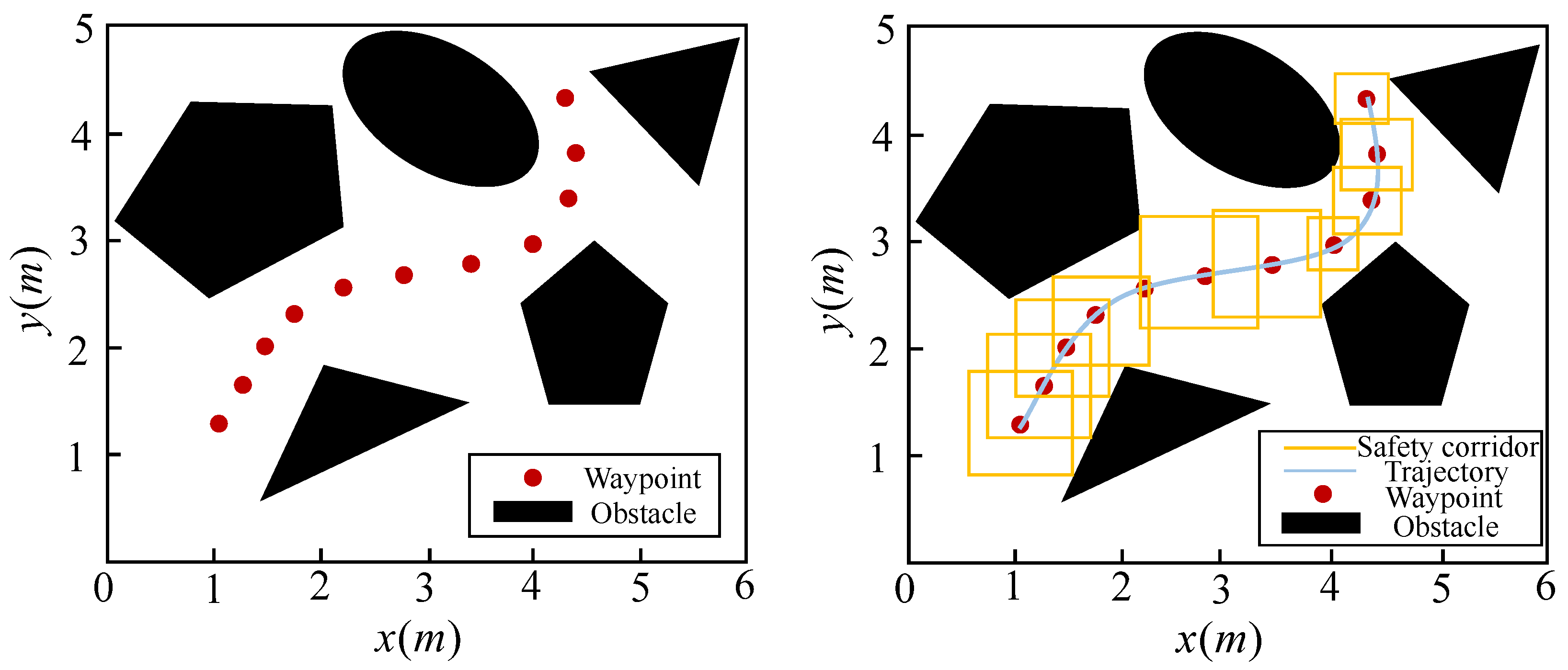
To avoid collision between trajectory and obstacles, it is necessary to limit the shape of the global trajectory, and the trajectory expected to be planned must be in a safe corridor. If the passable safe area is added to the path smoothing problem as a constraint, the trajectory will naturally be in the safe corridor. To impose security constraints, Bezier curves are introduced, and given in Equation (11):

$$E_j\left(t\right)=p_j^0{e}_n^0\left(t\right)+p_j^1{e}_n^1\left(t\right)+\cdots +p_j^n{e}_n^n\left(t\right),t\in [0,1]$$

(11)

where $p_j^i$ is the $i+1$ control points of a convex hull polygon, and $e_n^i\left(t\right)$ is a Berstein basis function, whose expression is defined as Equation (12):

$$e_n^i\left(t\right)=\left(\begin{array}{c}n\\ i\end{array}\right)·t^i·{(1-t)}^{n-i}$$

(12)

There is a transformation relationship between Bezier curve and polynomial curve, which can be described as Equation (13):

$$\sum _{i = 0}^n{p}_i\frac{n!}{(n-i)!i!}{(1-t)}^{n-i}{t}^i=q_0+q_{1}t+\cdots +q_n{t}^n$$

(13)

By limiting the control points of the Bezier curve, the shape of the curve can be controlled. The schematic diagram of the Bezier curve is shown in Figure 11, and the Bezier curve is limited in the area surrounded by the control points.

By deriving a 4-degree polynomial function, the expression of the change rate of jerk of any trajectory can be obtained as shown in Equation (14):

$$f^{\left(4\right)}\left(t\right)=\sum _{i \ge 4}i(i-1)(i-2)(i-3)t^{i-4}{q}_i$$

(14)

By substituting Equation (14) into Equation (10), the minimized snap minimization objective function of the whole trajectory is constructed, which is the integral of the square of the rate of change of jerk in the corresponding time segment of each trajectory, and is given in Equation (16).

$$Z\left(T\right)={\int }_{T_{j-1}}^{T_j}{\left(f^{\left(4\right)}\left(t\right)\right)}^2\mathrm{d}t$$

(15)

$$Z\left(T\right)={\left[\begin{array}{c}⋮\\ q_i\\ ⋮\end{array}\right]}^{\mathrm{T}}\left[\begin{array}{c}⋮\\ \cdots \frac{i(i-1)(i-2)(i-3)l(l-1)(l-2)(l-3)}{i+l-7}{T}^{i+l-7}\cdots \\ ⋮\end{array}\right]\left[\begin{array}{c}⋮\\ q_l\\ ⋮\end{array}\right]$$

(16)

In the formula, $q_i$, $q_l$ all denote the coefficients of each order of the polynomial trajectory, i and l are the orders of the trajectory polynomial, and j denotes the respective trajectory serial numbers in different time periods ($j=1,2,\cdots ,h$).

The snap minimization objective function of each trajectory is expressed in matrix form as Equation (17):

$$Z_j\left(T\right)=Q_j^T{L}_j{Q}_{\mathrm{j}}$$

(17)

where $Q_j$ is the coefficient matrix of the j-th trajectory polynomial; $L_j$ is the information matrix of locus polynomial in paragraph j.

Substituting formula (17) into formula (16), the snap minimization objective function of the whole trajectory is extended, as in Equation (18):

$$Z\left(T\right)=\sum _{j = 1}^h{Z}_j\left(T\right)=\sum _{j = 1}^h{Q}_j^T{L}_j{Q}_j={\left[\begin{array}{c}{Q}_1\\ ⋮\\ Q_j\\ ⋮\\ Q_h\end{array}\right]}_{j \times 8h}^{\mathrm{T}}{\left[\begin{array}{ccccc}{L}_1& 0& \cdots & 0& 0\\ 0& ⋮& 0& ⋮& 0\\ ⋮& 0& L_j& 0& ⋮\\ 0& ⋮& 0& ⋮& 0\\ 0& 0& \cdots & 0& L_N\end{array}\right]}_{8h \times 8h}{\left[\begin{array}{c}{Q}_1\\ ⋮\\ Q_j\\ ⋮\\ Q_h\end{array}\right]}_{8h \times j}$$

(18)

Therefore, the problem of minimizing the objective function is modeled as a mathematical quadratic programming (QP) problem. The standard mathematical form of a quadratic programming problem can be expressed as in Equation (19):

$$\begin{array}{cc}\underset{x}{minimize}& \frac{1}{2}{x}^{T}Px+q^{T}x\\ \mathrm{subject}\mathrm{to}& Gx-h\le 0,\\ & Ax-b=0\end{array}$$

(19)

where P is a symmetric matrix; G and A are n-dimensional real vectors; and q, h and b are real numbers. A standard quadratic programming problem consists of objective function, equality constraint, and inequality constraint.

After constructing the objective function to be optimized, because each trajectory is represented by two searched waypoints as endpoints and polynomial functions, as shown in Figure 12, the $q_{h-1}$ trajectory is connected with the $q_h$ trajectory at the $l_{h-1}$ point. In order to ensure that the trajectories with different parameters at both ends have better curvature connectivity at this point and make the final generated trajectory continuous, it is necessary to add continuity constraints and smoothness constraints to the constructed quadratic programming problem.

The continuity constraint of trajectory can be described as the position, velocity, acceleration, and jerk of the end of the j-segment trajectory and the head of the j + 1-segment trajectory being equal, respectively, which can ensure the continuity of the whole trajectory after optimization. Therefore, the continuity equality constraint is constructed as Equation (20):

$$f_j^{\left(k\right)}\left(T_j\right)=f_{j+1}^{\left(k\right)}\left(T_j\right)$$

(20)

where k is the order of derivative $(k=0,1,2,3)$, denoting position, velocity, acceleration, and jerk of each segment respectively; and $q_{j,i},q_{j+1l}$ represent the polynomial coefficients of the end of segment j and the beginning of segment $j+1$, respectively.

The trajectory is relatively stable at the starting point, the ending point, and the path connection point of every two trajectories. Also, the velocity, acceleration, and jerk of the trajectories at both ends should meet a certain value. Therefore, the smoothness equality constraint of the trajectory can be constructed according to the constraint condition in Equation (21):

$$f_j^{\left(k\right)}\left(T_j\right)=c_j^{\left(k\right)}$$

(21)

where c represents the x and y axes. To ensure the safety of the trajectory, a collision-free safe corridor is constructed according to the waypoint searched by the path planning algorithm, and the trajectory is generated in the corridor, so the trajectory must be safe and collision-free, as shown in the Figure 13. The security constraints are imposed as Equation (22):

$${\delta }_{\mu j}^{-}\le d_{\mu j}^{0,i}\le {\delta }_{\mu j}^{+}$$

(22)

where ${\delta }_{\mu j}^{-},{\delta }_{\mu j}^{+}$ is the maximum and minimum limit position of the safe corridor, and $d_{\mu j}^{l,i}$ is the control point of the Bezier curve of order r and degree i of the j-th trajectory on the $\mu$ axis.

The objective function based on minimizing snap is solved for the x-axis and y-axis, respectively, and the coefficients q of each trajectory satisfying the constraint conditions are obtained. The coefficients are then substituted into the state equations of each segment to solve the state variables in all directions of the whole trajectory, We apply the quadratic programming solver IPOPT library to perform online trajectory smoothing calculations. Finally, the trajectory to be optimized is obtained.

4. Experimental Evaluation

4.1. Simulation Experiment Analysis

To verify the effectiveness and robustness of the CRI-A* algorithm proposed in this paper, a comparative experiment between the traditional A* algorithm and CRI-A* algorithm was carried out. The simulation experiment was implemented on an Ubuntu 16.04 operating system, Robot Operating System (ROS), and C++ programming language on an I5-7200HQ CPU with 8 G memory portable computer. Simulation and visualization were implemented in Rviz. ROS system is an open-source robot meta-operating system, which is a robot software platform and provides a variety of programming platforms for developing applications for robots. Rviz is the visualization software of ROS; its characteristic is that it can express the data visually.

Four grid maps with different distributions of obstacles were established. Each grid map was given different starting points and target points. Relevant coordinate information are provided in

Table 3. Coordinate information of starting point and target point of different maps.

Map Number	Map Size/m	Start Point Coordinates	Target Point Coordinates
Map 1	50 × 50	(16, 8)	(39, 40)
Map 2	50 × 50	(14, 18)	(41, 33)
Map 3	50 × 50	(9, 17)	(80, 37)
Map 4	100 × 50	(7, 8)	(80, 45)

, and the corresponding simulation results are shown in Figure 14, Figure 15, Figure 16 and Figure 17. The maps are numbered Map1, Map2, Map3, and Map4, respectively. In each map image, black pixels represent obstacles; white dots are the waypoints obtained by the traditional A* algorithm; red dots are the waypoints obtained by CRI-A* algorithm; dark blue, light blue, and green represent the dangerous layer, the buffer layer, and the optimized trajectory, respectively. In the experiment, the path planned by the traditional A* algorithm has close proximity to obstacles. As such, there are collision risks in path tracking. In contrast, the path planned by CRI-A* algorithm ensures the safety of the robot during path tracking.

The simulation results of the above algorithms in four different map environments were analyzed, and the minimum distances between waypoints and obstacles planned by the two algorithms are recorded in

Table 4. Comparison of the shortest obstacle distance of two algorithms.

Map Number	Map Size/m	Traditional A* Distance/m	CRI-A* Distance/m	Distance Lifting Ratio	Number of Path Inflection Points	Smooth Inflection Point	Reduction Ratio
Map 1	50 × 50	1.67	2.23	49.29%	7	2	71.43%
Map 2	50 × 50	1.16	1.49	28.45%	6	1	83.33%
Map 3	100 × 50	1.29	1.86	44.18%	7	1	85.71%
Map 4	50 × 50	1.53	2.34	52.94%	5	2	60%

. By analyzing the data in the table, it can be concluded that the shortest distance between the path planned by the CRI-A* algorithm and the obstacles improved compared with traditional A*, with the highest lifting ratio of 52.94%, the lowest lifting ratio of 28.45%, and an average lifting ratio of 43.72%. After obtaining the waypoint, the number of inflection points was reduced through trajectory optimization; the highest reduction ratio is 85.71%, the lowest reduction ratio is 60%, and the average reduction rate is 75.12%.

The change in distance between path and obstacle and the number of inflection points in four experiments are plotted as a histogram, as shown in Figure 18. The analysis of experimental results shows that in a variety of different environments, the planned path is far away from obstacles, and the number of inflection points of the optimized trajectory is reduced. It can be seen that CRI-A* algorithm can ensure the security and smoothness of the planned paths, and also has good robustness.

4.2. Comparative Experiments with Existing Methods

To better validate the safety and smoothness of the path planning method proposed in this paper, we further reviewed relevant literature on risk-based path planning in ground mobile robots. An experimental comparison with existing excellent methods was made to prove the superiority of the algorithm proposed in this paper. CRI-A* was compared with the DSP method proposed by Karlsson et al. [24]. A grid map was selected, and different starting and target points were randomly selected. Five experiments were conducted, and the experimental results are shown in Figure 19, Figure 20, Figure 21, Figure 22 and Figure 23.

The shortest distance between the waypoints and obstacles planned by the two methods, as well as the number of inflection points on the path, were calculated and recorded in

Table 5. Comparison of experimental results between this method and DSP method.

Number of Experiments	DSP Distance/m	CRI-A* Distance/m	Distance Lifting Ratio	Number of Path Inflection Points	Smooth Inflection Point	Reduction Ratio
1	0.16	0.52	225%	4	2	50%
2	0.19	0.41	115.78%	6	1	83.33%
3	0.25	0.35	40%	3	2	33.33%
4	0.14	0.46	228.57%	5	2	60%
5	0.18	0.32	77.78%	4	1	75%

. The analysis of the data shows that the shortest distance between the waypoints and obstacles provided by the CRI-A* method increased by an average of 137.43%compared to the DSP method, and the number of inflection points decreased by 60.33%. To clearly display the experimental results, a bar chart is drawn, as shown in Figure 24. The bar chart proves the superiority of our proposed method over the DSP method in generating a smooth path for mobile robots. Though the path generated by the DSP method is comparatively shorter, our method outperforms it in the context of smoothness. Imperatively, path smoothness ensures that a robot is able to follow the global path generated during task execution. Additionally, smooth movements can promote affinity when robots operate in close proximity to humans, for instance, in the use of robots for home service or care.

4.3. Experimental Analysis of Real Environment

In order to further verify the effectiveness and robustness of our proposed method, this section uses actual robots to build indoor scenes for experimental verification.

The robot used in this experiment is TurtleBot2, a two-wheel differential-drive mobile robot designed and developed by Willow Garage Company, as shown in Figure 25. The robot is equipped with a Kobuki drive base, URG-04LX-UG01 2D lidar, and computer.

The experimental site is set up in an indoor environment. As shown in Figure 26, the experimental environment is a mouth-shaped area with a length of 12.8 m and a width of 2.4 m. The overall environment is complex, which meets the experimental requirements of home service robots in a complex environment.

The ROS platform was used to complete the map building of the experimental site. The map building process used Gmapping algorithm, which is a synchronous localization and mapping (SLAM) algorithm based on 2D lidar to complete grid map building, and converts the experimental site map into grid map. Gmapping algorithm is widely used because it has fewer computation requirements, high map accuracy, and a low requirement on lidar scanning frequency. The raster map based on the real environment is shown in Figure 27. In the figure, the black pixel areas represent obstacles, the gray areas represent areas of unknown occupancy, and white areas are unoccupied passable areas.

The traditional A* algorithm and the CRI-A* algorithm proposed in this paper are used for path planning. The experimental results are shown in Figure 28, Figure 29 and Figure 30. The dark blue area in Figure 29 is the dangerous layer, the light blue is the buffer layer, and the black curve in Figure 30 is the optimized trajectory. To clearly show the planned path, an enlargement is made to the right of the image.

By analyzing the experimental results, we can see that the waypoint planned by the traditional A* algorithm in the contrast area in the Figure 28 is close to the edge of the obstacle, although it does not collide with the obstacle. The radius of the actual robot is 150 mm and the resolution of the map in the graph is 0.05 m; that is, the side length of each grid is 50 mm, so the robot will collide with the obstacle when executing this path. After using the CRI-A* algorithm proposed in this paper and putting the physical size of the robot in to consideration, the width of the dangerous layer and buffer layer occupies six grids, which is physically equivalent to 300 mm. This provides an extra safe space for the robot and reduces collision risks.

Observing the path planned in Figure 29, we can see that each waypoint keeps a sufficiently safe distance from obstacles, and the distance in the contrast area is improved, thus ensuring the safety of the robot. To further analyze the experimental results clearly, the distance comparison map between traditional A* and CRI-A* waypoints and obstacles is drawn. The ordinate is the distance between waypoints and the nearest obstacles, and the abscissa is the transverse distance between each waypoint and the starting point. The curve of the distance between waypoints and obstacles changing with the transverse distance is drawn, and the safe distance is 2 times the diameter of the robot, that is, 60 cm. According to the analysis in Figure 31, the minimum distance from obstacles in the traditional A* algorithm is 5 cm, while the radius of a robot is 15 cm, which will collide with obstacles, and the distance between the path planned by traditional A* and obstacles is mostly less than the safe distance, which is very dangerous for robots. In contrast, the distance between the path and the obstacle is larger than the safe distance, which ensures the safety of the robot path planning and proves the effectiveness of the CRI-A* algorithm in the actual environment.

5. Conclusions and Future Work

The path obtained by the traditional global path search algorithm are usually placed in close proximity to obstacles, and thus introduces high navigation security risks. A path planning method for robots CRI-A* based on minimizing the danger index is proposed. After obtaining the waypoints, we use minimized snap based on the safe corridor to optimize the trajectory and improve the distance calculation method in the heuristic function. It is proven that the new distance calculation method reduces the number of search nodes by 23.5% on average; The proposed path planning algorithm is verified by using four different environment maps in the ROS simulation environment. The experimental results show that the proposed method improves the safety of path planning and the smoothness of the trajectory. Comparisons between the method proposed in this paper and the DSP method were made. The experimental results show that the relevant performance indicators improved. To verify the effectiveness of the algorithm in the real environment, an experimental environment was built and global path planning was carried out. The experimental results show that the proposed global path planning algorithm can ensure the safety and smoothness of the planned path.

This paper presents a secure and smooth global path planning framework. Though our proposed method is able to generate a safer path for robots, the global path generated is not the shortest path when compared with the DSP or A* methods. Also, if there are dynamic obstacles in the use scenario, a local dynamic path planning algorithm needs to be added. In future research work, we will investigate the perception and avoidance strategies of navigation systems towards dynamic obstacles, in order to improve their applicability to complex environments.