A Singular Perturbation Theory-Based Composite Control Design for a Pump-Controlled Hydraulic Actuator with Position Tracking Error Constraint

Abstract

Pump-controlled hydraulic actuators (PHAs) contain slow mechanical and fast hydraulic dynamics, and thus singular perturbation theory can be adopted in the control strategies of PHAs. In this article, we develop a singular perturbation theory-based composite control approach for a PHA with position tracking error constraint. Disturbance observers (DOBs) are used to estimate the matched and mismatched uncertainties for online compensation. A sliding surface-like error variable is proposed to transform the second-order mechanical subsystem into a first-order error subsystem. Consequently, the position tracking error constraint of the PHA is decomposed into the output constraint of the first-order error subsystem and the stabilizing of the first-order hydraulic subsystem. Slow and fast control laws can be easily designed without using the backstepping technique, thus simplifying the control design and reducing the computational burden to a large extent. Theoretical analysis verifies that desired stability properties can be achieved by an appropriate selection of the control parameters. Simulations and experiments are performed to confirm the efficacy and practicability of the proposed control strategy.

1. Introduction

Pump-controlled hydraulic actuators (PHAs) have been widely used in industrial applications [1,2,3] due to their high power-to-weight ratio, energetic efficiency, simple structure, compactness, and ease of maintenance [4,5,6]. However, ensuring high-performance output tracking control is a primary demand for PHAs. Unfortunately, parametric uncertainties, sophisticated friction force, and other disturbances can degrade control performance. Load disturbances, for example, not only affect velocity dynamics but can also cause piston vibrations and pressure fluctuations. To mitigate these effects, many advanced control strategies have been successfully applied in hydraulic systems, such as sliding mode control [7], robust adaptive control [8], and robust integral of the sign of the error (RISE) [9]. While these methods are effective, they rely on high gains to achieve uncertainty attenuation, which may result in large design conservativeness and amplify the noise effect.

As an alternative, observer-based methods, such as disturbance observer (DOB) [10] and extended state observer (ESO) [11], provide estimates of uncertainties for online compensation in controller synthesis, thus avoiding high robust feedback gains and reducing design conservativeness. Observer-based methods have drawn increasing attention in recent years. In [12], a disturbance observer-based state estimator (DOBSE) was designed to asymptotically estimate the disturbance without specifying the boundedness of the disturbance. In [13], a fixed-time disturbance observer was developed to asymptotically estimate the disturbance within a given period. In [14], two ESOs were coordinated to concurrently estimate the unavailable states and matched and mismatched uncertainties with only output information. In [15], a finite-time extended state observer (FTESO) was proposed to achieve the asymptotic estimation of disturbances and unavailable states in finite time. In [16], extended sliding mode observers (ESMOs) were proposed to achieve faster convergence, higher accuracy, and better robustness against uncertainties by comparison with traditional ESOs.

Aside from uncertainty attenuation, the outputs of PHAs are often required to track their desired trajectories within an acceptable range in the whole operation process. To achieve the output tracking error constraint, a barrier Lyapunov function (BLF) [17] was proposed in the backstepping framework for strict feedback nonlinear systems. The BLF contains a natural logarithm function of the output tracking error such that the BLF will be unbounded if the output tracking error violates the prescribed bound. Thus, the output tracking error constraint is achieved by designing a proper controller to guarantee the boundedness of the BLF. BLF-based control approaches have been widely applied in hydraulic systems, and some examples can be found in [18,19,20].

Based on the above discussion, we can design a BLF-based backstepping controller with observers to guarantee the output tracking error constraint of a PHA subject to matched and mismatched uncertainties. However, the drawback of this method is that the backstepping technique needs the calculation of the time derivatives of intermediate virtual control laws, which becomes extremely complicated in high-order systems. Moreover, the incorporated BLF exaggerates the design complexity and computational burden. Although dynamic surface control (DSC) [21] can avoid the problem of “explosion of complexity”, the introduced filters also complicate the control structure and cause phase lag [22]. Therefore, it is of practical importance to develop a BLF-based output tracking error constraint control method for PHAs without using the backstepping technique.

In this paper, we present a simple control design scheme for a PHA to achieve position tracking error constraint and uncertainty compensation without the backstepping technique. It starts with decomposing the PHA into slow mechanical and fast hydraulic subsystems from the viewpoint of time scale separation [23]. Owing to this, singular perturbation theory [24] can be utilized in the control synthesis of the PHA. We decompose the actual control law into slow and fast components and then stipulate a restrictive condition to make them decoupled to control the corresponding subsystems. Consequently, the control task is reduced to investigating the two reduced-order subsystems.

The mechanical subsystem of the PHA is in a second-order integral chain form to describe the position and velocity dynamics. To achieve position tracking error constraint, the backstepping technique is still required in the synthesis of the slow control law. To circumvent this, we propose a sliding surface-like error variable to transform the second-order mechanical subsystem into a first-order error subsystem. Via this transformation, the position tracking error constraint of the PHA is equivalent to the output constraint of the transformed first-order error subsystem. Therefore, a BLF-based slow control law can be easily designed without any intermediate virtual control law. Two DOBs are combined to estimate the uncertainties for online compensation. The fast control law is required to ensure the uniform stability of the first-order hydraulic subsystem. Compared with backstepping-based methods, the proposed composite control method is low-complexity and straightforward. Stability analysis via singular perturbation theory reveals that the position tracking error constraint and desired stability properties can be obtained by a proper selection of the control parameters.

The main contributions of this article are generalized below:

(1)

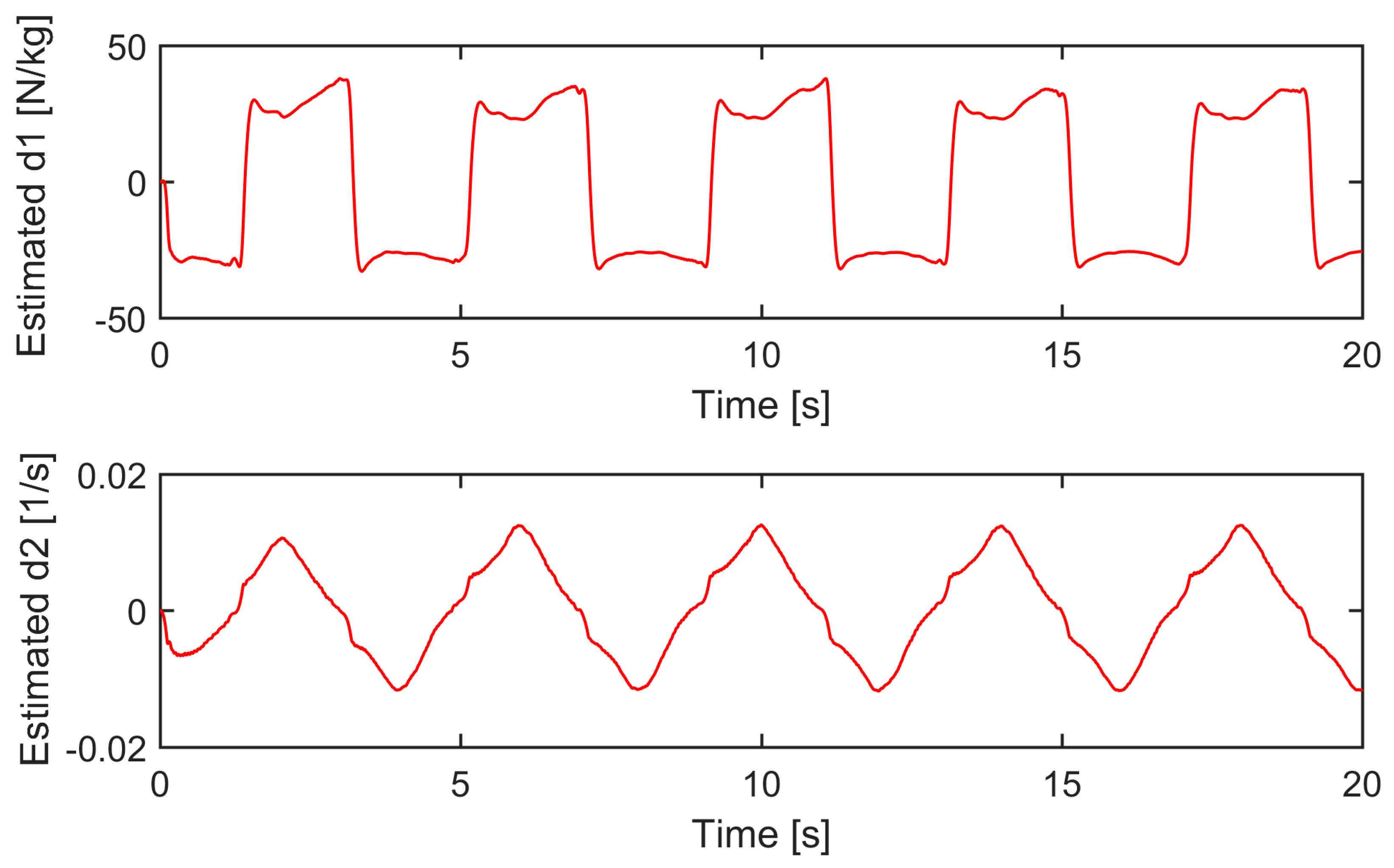
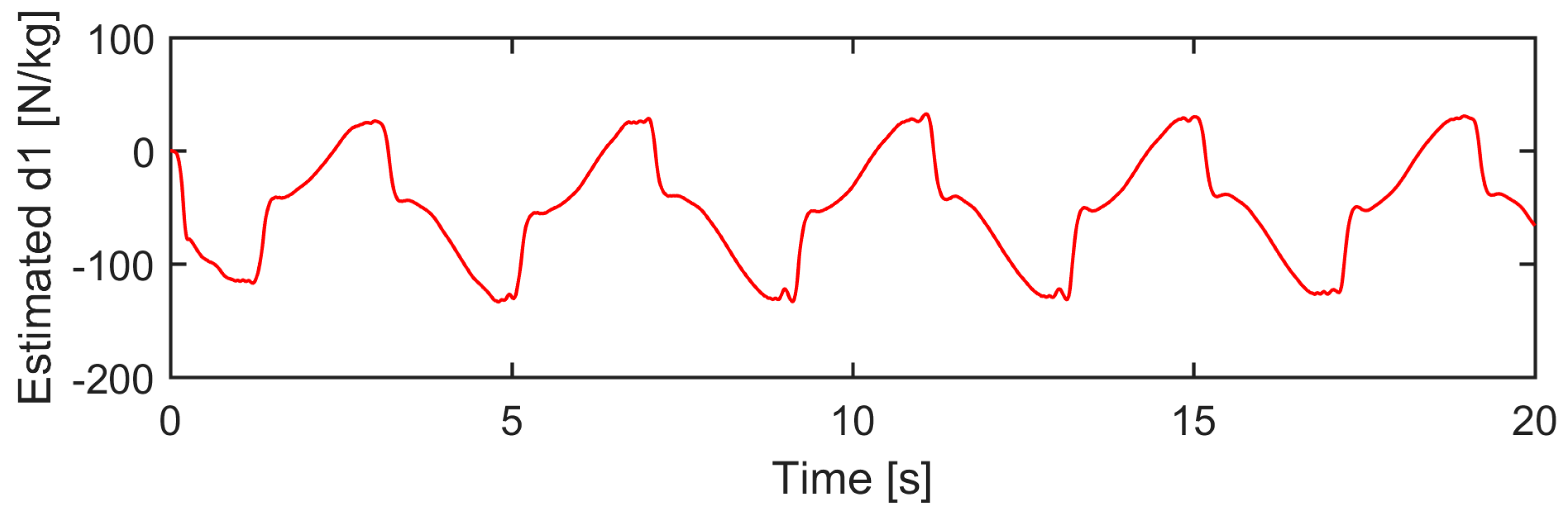
Position tracking error constraint is investigated for a PHA subject to uncertainties. Two DOBs are incorporated to provide estimates of the matched and mismatched uncertainties.

(2)

Unlike the existing works [14,25,26], the PHA is decomposed into slow mechanical and fast hydraulic subsystems from a two-time scale perspective. Therefore, the control task is reduced to investigating the two reduced-order subsystems.

(3)

Compared with the BLF-based control [27,28,29], the proposed sliding surface-like error variable transforms the position tracking error constraint of the third-order PHA into the output constraint of a first-order error subsystem and the stabilizing of the first-order hydraulic subsystem. Consequently, a composite controller can be easily designed without the use of the backstepping technique.

(4)

The proposed control approach has a simple control structure, low computational burden, and satisfactory control accuracy, which makes it promising in industrial applications.

The remainder of this article is organized as follows. The system is modeled in Section 2. In Section 3, the singular perturbation theory-based composite control design is proposed in detail. The closed-loop system stability analysis is conducted in Section 4. Simulation and experimental validation are displayed in Section 5. Section 6 concludes this paper.

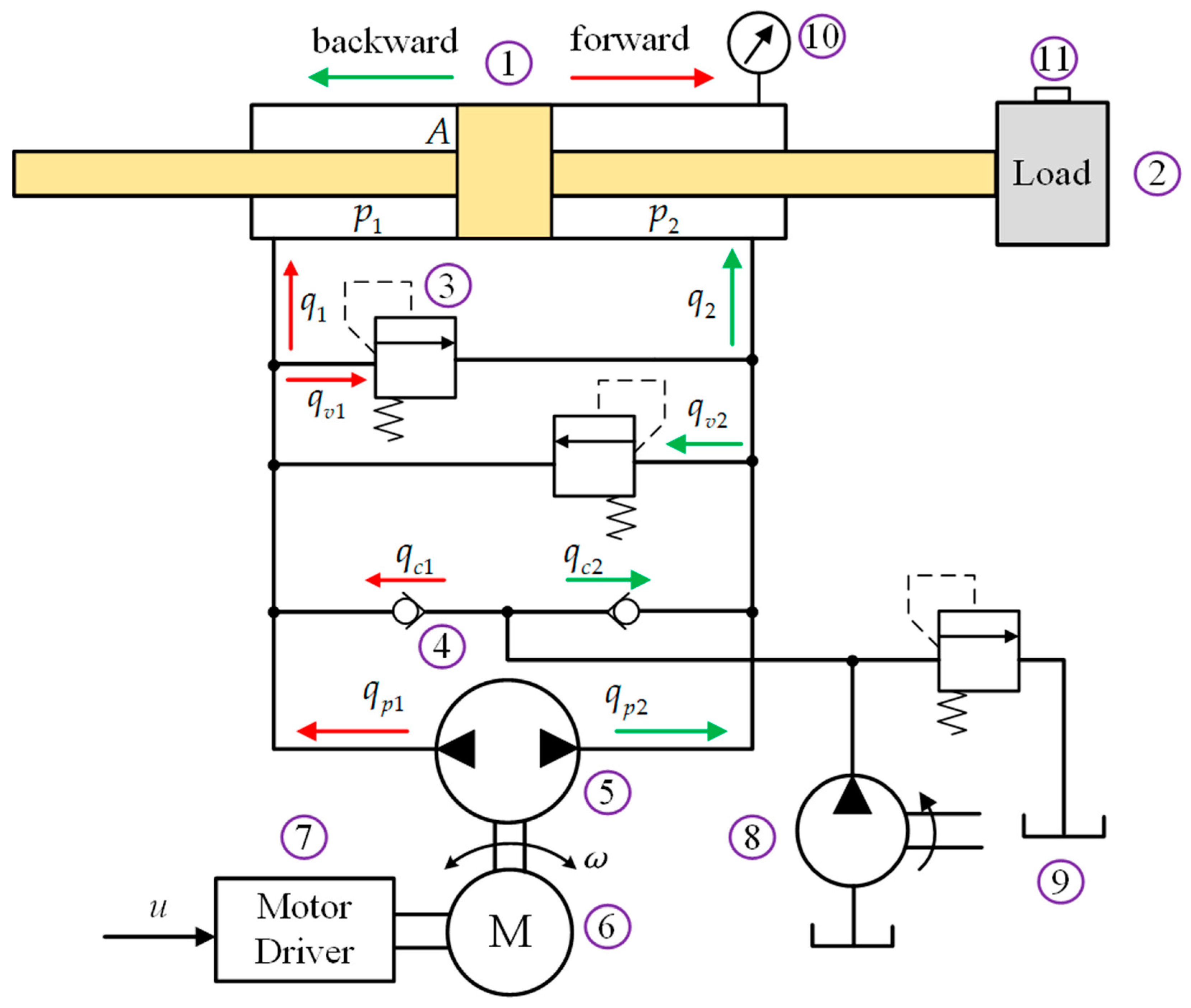
2. System Modeling

The schematic diagram of a PHA is depicted in Figure 1. As seen, the control voltage acts on the motor driver, and the servo motor drives the bidirectional pump to rotate. The pump outputs pressure oil to force the movement of the piston rod of the cylinder. Relief valves are installed to restrict the maximum working pressure. A charging circuit is constructed to compensate for the external leakage. A load is connected to the piston rod. Pressure sensors and a rotary encoder are installed to record the pressures inside the chambers of the cylinder and the position of the piston rod, respectively.

The dynamics of the piston rod can be determined by Newton’s law:

$$m\ddot{y}=A\left(p_1-p_2\right)-F_f-F_l+F_d$$

(1)

where m is the total mass of the piston rod and the connected load; y is the position of the piston rod; A is the ram area of the cylinder; p₁ and p₂ are the pressures inside the two chambers of the cylinder; F_f represents the sophisticated nonlinear friction, which comprises linear viscous friction and other nonlinear elements; F_l is the load force; and F_d denotes the lumped uncertainties due to parametric uncertainties, unmodeled nonlinearities, and load disturbances.

Neglecting the external leakage, the pressure dynamics in both chambers of the cylinder are given by [30]:

$${\dot{p}}_1=\frac{{\beta }_e}{V_{01}+Ay}\left[-A\dot{y}-C_{tlc}\left(p_1-p_2\right)+q_1+q_{n1}\right]$$

(2)

$${\dot{p}}_2=\frac{{\beta }_e}{V_{02}-Ay}\left[A\dot{y}+C_{tlc}\left(p_1-p_2\right)+q_2+q_{n2}\right]$$

(3)

where V₀₁ and V₀₂ represent the initial control volumes of each chamber and the volumes of the connecting pipelines; β_e is the effective bulk modulus; C_tlc denotes the total leakage coefficient of the cylinder; q₁ and q₂ denote the flow rates into the two chambers of the cylinder; and q_n1 and q_n2 represent parametric uncertainties and modeling errors.

It is inferred from Figure 1 that the flow rates q₁ and q₂ are determined by:

$$q_1=q_{p1}+q_{c1}-q_{v1}$$

(4)

$$q_2=q_{p2}+q_{c2}-q_{v2}$$

(5)

where q_p1 and q_p2 are pump flow rates; q_c1 and q_c2 are charging flow rates; and q_v1 and q_v2 are the flow rates through the relief valves.

We should note that in normal operation, the system pressure does not violate the safety limit value of the relief valves. Therefore, there is no flow rate through the relief valves, which means that:

$$q_{v1}=q_{v2}=0$$

(6)

Referring to [31], the pump flow rate can be expressed by:

$$q_{p1}=-q_{p2}=D\omega -C_{tlp}\left(p_1-p_2\right)+q_{n3}$$

(7)

where D is the pump volumetric displacement; ω is the rotary speed; C_tlp represents the total leakage coefficient of the pump; and q_n3 denotes the parametric uncertainties and modeling error.

Since the motor is directly connected to the pump, the pump rotational dynamics can be determined by the following equilibrium equation of moments [32]:

$$J\dot{\omega }=T_m-B\omega -T_d-D(p_1-p_2)$$

(8)

where T_m is the torque generated by the servo motor; J represents the inertia of the motor/pump; B is the coefficient of friction and viscosity; and T_d represents the static friction at the pump/motor interface.

In this study, the servo motor has an inner velocity closed-loop and fast control response; therefore, the rotational dynamics can be simplified to a static equation [31,33,34]:

$$\omega =K_{m}u$$

(9)

where K_m is the scale input coefficient of the servo motor and u is the voltage input.

Defining the state variables as $X={[x_1,x_2,x_3]}^T={[y,\dot{y},p_1-p_2]}^T$ and combining (1)–(9), the mathematical model of the studied PHA is given by:

$$\begin{array}{c} {\dot{x}}_1=x_2\\ {\dot{x}}_2=a_1{x}_3+d_1\\ \epsilon {\dot{x}}_3=b_{1}u-b_2{x}_2-b_3{x}_3+d_2\\ \hspace{1em}y=x_1\end{array}$$

(10)

where a₁ = A/m, ε = 1/β_e, b₁ = DK_m [1/(V₀₁ + Ax₁) + 1/(V₀₂ − Ax₁)], b₂ = A [1/(V₀₁ + Ax₁) + 1/(V₀₂ − Ax₁)], b₃ = C_t [1/(V₀₁ + Ax₁) + 1/(V₀₂ − Ax₁)], C_t = C_tlc + C_tlp; the mismatched uncertainties d₁ = (−F_f − F_l + F_d)/m; and the matched uncertainties d₂ = (q_n1 + q_n3 + q_c1)/(V₀₁ + Ax₁) − (q_c2 + q_n2 − q_n3)/(V₀₂ − Ax₁). Note that since V₀₁ and V₀₂ contain the volumes of the pipelines, no matter where the piston rod is, b₁, b_2, and b₃ are always positive.

Generally speaking, β_e reaches an order of magnitude of 10⁹ or higher; thus, ε is a positive constant much smaller than 1. It implies that the system (10) is in a singularly perturbed form, and thus singular perturbation theory can be utilized in control design.

The objective of this article is to develop a continuous control law u such that:

(1)

The position of the piston rod tracks a given reference trajectory within an expected range, i.e.,:

$$\left|y(t)-y_d(t)\right|<k_b,\hspace{1em}\forall t\ge 0$$

(11)

where y_d is a given reference trajectory and k_b is a prescribed bound.

(2)

A satisfactory final position tracking error can be obtained.

Assumption 1: 

The desired trajectory y_d(t) and its derivatives up to the third order are bounded and continuous.

Assumption 2: 

The uncertainties d₁ and d₂ are bounded and there are positive constants Δ₁ and Δ₂ such that:

$$\left|{\dot{d}}_1\right|\le {\Delta }_1,\hspace{1em}\left|{\dot{d}}_2\right|\le {\Delta }_2$$

(12)

Remark 1: 

Note that the lumped uncertainties d₁ involve nonlinear friction F_f, which is normally expressed by a discontinuous model to describe the friction effect that the friction cutovers around zero velocity. For instance, the most widely used discontinuous friction model [35] is defined by:

$$F_f=\left(f_s-f_c\right)\exp \left[-{\left(\left|x_2\right|/v_s\right)}^m\right]\mathrm{sign}(x_2)+f_c\mathrm{sign}(x_2)+f_v{x}_2$$

(13)

where v_s is the Stribeck velocity; f_s is the stiction force; m usually takes the value of 1 or 2; and f_c and f_v are the Coulomb friction coefficient and viscous coefficient, respectively.

However, the discontinuity leads to the friction force being non-differentiable on zero velocity, which impedes the development of friction compensation approaches in hydraulic systems. To handle this problem, a smooth nonlinear friction model is proposed in [36] and is defined by:

$$F_f={\gamma }_1\left[\tanh ({\gamma }_{2}v)-\tanh ({\gamma }_{3}v)\right]+{\gamma }_4\tanh ({\gamma }_{5}v)+{\gamma }_{6}v$$

(14)

to represent various friction effects, in which γ₁–γ₆ are positive parameters, the term tanh(γ₂v)-tanh(γ₃v) stands for the Stribeck effect, the term γ₄tanh(γ₅v) represents the Coulomb friction, the term γ₆v denotes the viscous friction, and γ₁ + γ₄ is the stiction force.

Theoretical analysis has been performed in [37] to prove that a proper selection of the parameters γ₁–γ₆ such that:

$${\gamma }_1=f_s-f_c, {\gamma }_2>{\gamma }_3, {\gamma }_2\gg 0, {\gamma }_3=1/v_s, {\gamma }_4=f_c, {\gamma }_5\gg 0, {\gamma }_6=f_v$$

(15)

then, the smooth friction model (14) behaves similarly to the discontinuous friction model (13).

In addition, verification experiments have been conducted in [38] to reveal that the smooth friction model (14) can give an excellent description of the actual friction. Therefore, similar to [37,39,40], it is acceptable and practicable to employ this smooth nonlinear friction model (14) to describe the actual friction in the PHA system. Consequently, the boundedness of the first-order derivative of the nonlinear friction is guaranteed.

Remark 2: Assumption 1 

is frequently made in the tracking control of nonlinear systems [13,14,41]. This assumption ensures the smoothness of the reference trajectories, which prevents the abrupt vibrations of system states [13]. Assumption 2 is generally required in observer-based control approaches [14,29,42,43]. From a practical point of view, it takes into account that the energy and the change rate of practical nonlinear dynamics are limited. Therefore, Assumptions 1–2 are reasonable.

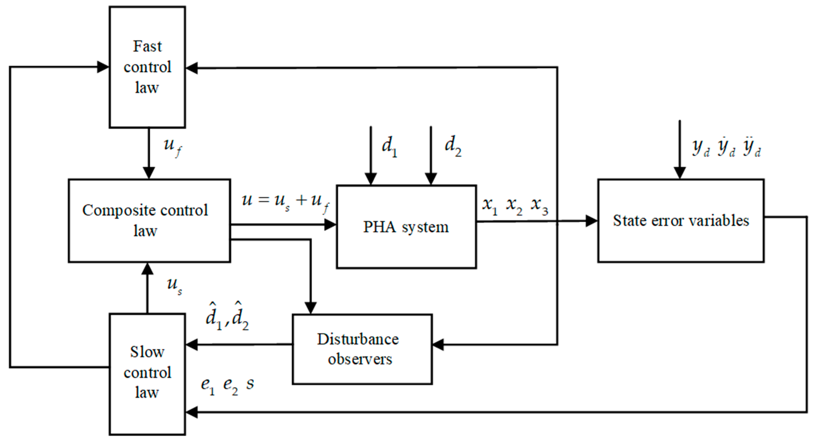
3. Singular Perturbation Theory-Based Composite Control Design

3.1. Design of the DOBs

In this paper, two DOBs are designed, as follows, to estimate the matched and mismatched uncertainties:

$$\begin{array}{l}{\widehat{d}}_1=l_1\left(x_2-{\widehat{x}}_2\right),\hspace{1em}\hspace{1em}{\dot{\widehat{x}}}_2=a_1{x}_3+{\widehat{d}}_1\\ {\widehat{d}}_2=l_2\left(\epsilon x_3-\epsilon {\widehat{x}}_3\right),\hspace{1em}\epsilon {\dot{\widehat{x}}}_3=b_{1}u-b_2{x}_2-b_3{x}_3+{\widehat{d}}_2\end{array}$$

(16)

where l₁ and l₂ > 0 are the observer gains.

Define the estimation errors as:

$${\tilde{d}}_1=d_1-{\widehat{d}}_1,\hspace{1em}{\tilde{d}}_2=d_2-{\widehat{d}}_2$$

(17)

It is obtained from (16) that:

$$\begin{array}{l}{\dot{\tilde{d}}}_1=-l_1{\tilde{d}}_1+{\dot{d}}_1\\ {\dot{\tilde{d}}}_2=-l_2{\tilde{d}}_2+{\dot{d}}_2\end{array}$$

(18)

Since the observer gains l₁ and l₂ in (16), and the perturbation parameters ε are positive constants, there are always positive constants h₁ and h₂ such that:

$$\epsilon h_1{l}_1=\epsilon h_2{l}_2=1$$

(19)

Then, the estimation error dynamics is rewritten as:

$$\begin{array}{l}\epsilon {\dot{\tilde{d}}}_1=-\frac{1}{h_1}{\tilde{d}}_1+\epsilon {\dot{d}}_1\\ \epsilon {\dot{\tilde{d}}}_2=-\frac{1}{h_2}{\tilde{d}}_2+\epsilon {\dot{d}}_2\end{array}$$

(20)

3.2. Singular Perturbation Theory-Based Composite Controller Design

The mathematical model of the PHA (10) and the estimation error dynamics (20) can be represented in the following singularly perturbed form:

$$\dot{\xi }=\varphi (t,\xi ,\lambda )$$

(21)

$$\epsilon \dot{\lambda }=\psi (t,\xi ,\lambda ,u,\epsilon )$$

(22)

where:

$$\xi =\left[\begin{array}{c}{x}_1\\ x_2\end{array}\right], \lambda =\left[\begin{array}{c}{x}_3\\ {\tilde{d}}_1\\ {\tilde{d}}_2\end{array}\right], \varphi (t,\xi ,\lambda )=\left[\begin{array}{c}{x}_2\\ a_1{x}_3+d_1\end{array}\right], \psi (t,\xi ,\lambda ,u,\epsilon )=\left[\begin{array}{c}{b}_{1}u-b_2{x}_2-b_3{x}_3+{\widehat{d}}_2+{\tilde{d}}_2\\ -h_1^{-1}{\tilde{d}}_1+\epsilon {\dot{d}}_1\\ -h_2^{-1}{\tilde{d}}_2+\epsilon {\dot{d}}_2\end{array}\right]$$

(23)

Introduce a new time scale τ = t/ε and the system dynamics (21)–(22) can be represented in τ time scale as:

$$\frac{d\xi }{d\tau }=\epsilon \varphi (t,\xi ,\lambda ), \frac{d\lambda }{d\tau }=\psi (t,\xi ,\lambda ,u,\epsilon )$$

(24)

As seen, the dynamics of ξ in the τ time scale are scaled down by the small parameter ε. Therefore, ξ dynamics can be regarded as a slow subsystem and λ dynamics as a fast subsystem.

Owing to this, singular perturbation theory can be adopted to obtain a reduced-order model, which is in an integral chain form to facilitate control design and uncertainty compensation. It starts with the assumption that ε = 0, and then (22) becomes an algorithm equation:

$$\psi (t,\xi ,\lambda ,u,0)=0$$

(25)

The solution $\overline{\lambda }$ is called the “quasi-steady-state” of the fast variable λ, which can be calculated as:

$$\overline{\lambda }={\left[{\overline{\lambda }}_1,{\overline{\lambda }}_2,{\overline{\lambda }}_3\right]}^T={\left[\begin{array}{c}\frac{1}{b_3}(b_{1}u-b_2{x}_2+{\widehat{d}}_2)\hspace{1em}0\hspace{1em}0\end{array}\right]}^T$$

(26)

Introduce an error:

$$\eta =\lambda -\overline{\lambda }$$

(27)

to represent the discrepancy between the actual states and their quasi-steady-states. It is known from (26)–(27) that:

$$x_3={\overline{\lambda }}_1+{\eta }_1, {\tilde{d}}_1={\eta }_2, {\tilde{d}}_2={\eta }_3$$

(28)

Then, the PHA system (10) is transformed into the following singular perturbed system in the (ξ, η₁) coordinates:

$$\begin{array}{l}\dot{\xi }=\left[\begin{array}{c}{x}_2\\ a_1{\overline{\lambda }}_1+a_1{\eta }_1+d_1\end{array}\right]=\left[\begin{array}{c}{x}_2\\ \frac{a_1{b}_1}{b_3}u-\frac{a_1{b}_2}{b_3}{x}_2+a_1{\eta }_1+d_1+\frac{a_1}{b_3}{\widehat{d}}_2\end{array}\right]\\ \epsilon {\dot{\eta }}_1=-b_3{\eta }_1+{\eta }_3-\epsilon {\dot{\overline{\lambda }}}_1\end{array}$$

(29)

Therefore, the singular perturbation theory reduces the control problem of the third-order PHA to that of a second-order integral chain system. However, since u is excluded from the η₁ dynamics, the convergence performance of η₁ cannot be arbitrarily adjusted.

Motivated by [24], we develop a singular perturbation theory-based composite control design method with:

$$u=u_s+u_f$$

(30)

where u_s and u_f represent its slow and fast control laws, respectively. We intend to decouple the control laws and let them act on the corresponding subsystems. It is feasible by stipulating a restrictive condition that:

$$u_f=0 \mathrm{for} \eta =0$$

(31)

By repeating the procedure in (25), we can obtain that the quasi-steady-state $\overline{\lambda }$ that becomes the solution of $\psi (t,\xi ,\overline{\lambda },u_s,0)=0$. It is easy to obtain that:

$$\overline{\lambda }={\left[\begin{array}{c}\frac{1}{b_3}\left(b_1{u}_s-b_2{x}_2+{\widehat{d}}_2\right)\hspace{1em}0\hspace{1em}0\end{array}\right]}^T$$

(32)

Recall that $x_3={\overline{\lambda }}_1+{\eta }_1$. This modification (32) makes the PHA system (10) transform into the following singularly perturbed system:

$$\dot{\xi }=\left[\begin{array}{c}{x}_2\\ a_1{\overline{\lambda }}_1+a_1{\eta }_1+d_1\end{array}\right]=\left[\begin{array}{c}{x}_2\\ \frac{a_1{b}_1}{b_3}{u}_s-\frac{a_1{b}_2}{b_3}{x}_2+a_1{\eta }_1+d_1+\frac{a_1}{b_3}{\widehat{d}}_2\end{array}\right]$$

(33)

$$\begin{array}{cc}\epsilon {\dot{\eta }}_1& =\epsilon {\dot{x}}_3-\epsilon {\dot{\overline{\lambda }}}_1=b_1{u}_f+(b_1{u}_s-b_2{x}_2-b_3{\overline{\lambda }}_1+{\widehat{d}}_2)+{\tilde{d}}_2-b_3{\eta }_1-\epsilon {\dot{\overline{\lambda }}}_1\\ & =b_1{u}_f-b_3{\eta }_1+{\eta }_3-\epsilon {\dot{\overline{\lambda }}}_1\end{array}$$

(34)

As seen, the slow control law u_s is moved to the slow ξ subsystem by ${\overline{\lambda }}_1$, while the fast control law u_f is retained in the fast η₁ subsystem. Therefore, they can be separately designed for different control objectives.

The slow control law u_s is designed to achieve the position tracking error constraint of the reduced-order integral chain system (33). We first define a tracking error vector $e={[e_1,e_2]}^T$, in which:

$$e_1=y-y_d, e_2=x_2-{\dot{y}}_d$$

(35)

Its dynamics are given by:

$$\dot{e}=\left[\begin{array}{c}{e}_2\\ \frac{a_1{b}_1}{b_3}{u}_s-\frac{a_1{b}_2}{b_3}{x}_2+a_1{\eta }_1+d_1+\frac{a_1}{b_3}{\widehat{d}}_2-{\ddot{y}}_d\end{array}\right]$$

(36)

To constrain the position tracking error e₁ within the prescribed bound k_b, where $k_b>\left|e_1(0)\right|$, we first propose a sliding surface-like error variable:

$$s=r{e}_1+e_2$$

(37)

where r > 0 is a design parameter.

Lemma 1: 

For any $k_b>\left|e_1(0)\right|$, if s(t) satisfies $\left|s(t)\right|<\rho , \forall t\ge 0$, where ρ is an arbitrarily constant satisfying:

$$0<\rho <r(k_b-\left|e_1(0)\right|)$$

(38)

Then:

$$\left|e_1(t)\right|<k_b,\hspace{1em}\left|e_2(t)\right|<r\left(2k_b-\left|e_1(0)\right|\right)$$

(39)

$\forall t\ge 0$.

Proof. 

From (36) and (37), we have:

$${\dot{e}}_1=-r{e}_1+s$$

(40)

The solution of (40) is:

$$e_1(t)=e^{-rt}{e}_1(0)+{\displaystyle {\int }_0^t{e}^{-r(t-\gamma )}s(\gamma )}d\gamma$$

(41)

Assume that $\left|s(t)\right|<\rho , \forall t\ge 0$, (41) can be augmented to:

$$\left|e_1(t)\right|\le \left|e_1(0)\right|+{\displaystyle {\int }_0^t{e}^{-r(t-\gamma )}}\left|s(\gamma )\right|d\gamma \le \left|e_1(0)\right|+\frac{\rho }{r}-\frac{\rho }{r}{e}^{-rt}$$

(42)

Applying the inequality (38) to (42), we can obtain: $\left|e_1(t)\right|<k_b, \forall t\ge 0$.

In addition, since $e_2=s-r{e}_1$, we have:

$$\left|e_2(t)\right|\le \left|s(t)\right|+r\left|e_1(t)\right|<\rho +r{k}_b<r(2k_b-\left|e_1(0)\right|)$$

(43)

$\forall t\ge 0$. □

Remark 3: 

It can be seen that the bounds k_b and ρ depend on the initial condition e₁(0), which means that they may be chosen with different values when tracking different reference trajectories. It is the limitation of the proposed sliding surface-like error variable.

It can be inferred from Lemma 1 that the position tracking error constraint of (33)–(34) is equivalent to the construction of u_s to guarantee that $\left|s(t)\right|<\rho$.

Differentiating s with respect to t, we obtain the following first-order error subsystem:

$$\dot{s}=r{e}_2+\frac{a_1{b}_1}{b_3}{u}_s-\frac{a_1{b}_2}{b_3}{x}_2+a_1{\eta }_1+d_1+\frac{a_1}{b_3}{\widehat{d}}_2-{\ddot{y}}_d$$

(44)

To achieve the output constraint of (44), we design a BLF-based slow control law:

$$u_s=\frac{b_3}{a_1{b}_1}\left[-k_{1}s+\frac{a_1{b}_2}{b_3}{x}_2+{\ddot{y}}_d-{\widehat{d}}_1-\frac{a_1}{b_3}{\widehat{d}}_2-r{e}_2-\frac{s}{4\left({\rho }^2-s^2\right)}\left(a_1^2+1\right)\right]$$

(45)

where k₁ > 0 is a feedback gain and $-\frac{s}{4\left({\rho }^2-s^2\right)}\left(a_1^2+1\right)$ is a robust term to suppress the effects of a₁η₁ and η₂.

u_f is designed to make the η₁ subsystem converge fast and finally converge to a small region around zero. As a result, the effect of the term a₁η₁ on the ξ subsystem can be made small. In the meantime, u_f must satisfy the restrictive condition (31). To this end, u_f can be designed as:

$$u_f=-\frac{k_2}{b_1}{\eta }_1$$

(46)

where k₂ > 0 is the feedback gain.

The control framework of the closed-loop system is presented in Figure 2.

Remark 4: 

The singular perturbation theory introduces a two-time scale perspective to decompose the original third-order PHA into a second-order integral chain slow subsystem and a first-order fast subsystem. A singular perturbation theory-based composite control method is developed to separate the control law into fast and slow components, which function as the control inputs of the corresponding subsystems by stipulating a restrictive condition. A sliding surface-like error variable is proposed to further simplify the control task to the output constraint control of a transformed first-order error subsystem and stabilize the first-order fast subsystem. Consequently, the control laws can be easily designed without any intermediate virtual control law. On the contrary, BLF-based backstepping controllers require a calculation of the time derivatives of virtual control laws, which becomes extremely complicated in high-order systems. Therefore, the proposed control approach greatly simplifies the controller design and reduces the computational burden.

4. Closed-Loop System Stability Analysis via Singular Perturbation Theory

Combing (20), (28), (34), and (44)–(46), the closed-loop system can be represented as the following singularly perturbed form:

$$\begin{array}{c}\dot{s}=f(t,s,\eta ,\epsilon )\\ \epsilon \dot{\eta }=g(t,s,\eta ,\epsilon )\end{array}$$

(47)

where: $f(t,s,\eta ,\epsilon )=-k_{1}s+a_1{\eta }_1+{\eta }_2-\frac{s}{4\left({\rho }^2-s^2\right)}\left(a_1^2+1\right)$,

$$g(t,s,\eta ,\epsilon )=\left[\begin{array}{c}-(k_2+b_3){\eta }_1+{\eta }_3-\epsilon {\dot{\overline{\lambda }}}_1\\ -\frac{1}{h_1}{\eta }_2+\epsilon {\dot{d}}_1\\ -\frac{1}{h_2}{\eta }_3+\epsilon {\dot{d}}_2\end{array}\right]$$

(48)

The stability analysis for the singularly perturbed system (47) is conducted in two steps:

(1) Find two Lyapunov functions to investigate the stability properties of the boundary layer system and the reduced system;

(2) Use the sum of the aforementioned Lyapunov functions as a composite Lyapunov function candidate to analyze the closed-loop system stability.

Step 1: The boundary layer system is obtained by setting ε = 0 in the τ time scale so that:

$$\frac{d\eta }{d\tau }=g(t,s,\eta ,0)=A_{\eta }\eta +B_{\eta }\eta$$

(49)

where: $A_{\eta }=\left[\begin{array}{ccc}-(k_2+b_3)& 0& 0\\ 0& -h_1^{-1}& 0\\ 0& 0& -h_2^{-1}\end{array}\right]$, $B_{\eta }=\left[\begin{array}{ccc}0& 0& 1\\ 0& 0& 0\\ 0& 0& 0\end{array}\right]$.

Theorem 1: 

The boundary layer system (49) is asymptotically stable if the control parameters k₂, h₁, and h₂ are chosen such that $1-{‖P_{\eta }‖}_2>0$, where P_η is a symmetric positive definite matrix satisfying $P_{\eta }{A}_{\eta }+A_{\eta }^T{P}_{\eta }=-2I.$

Proof. 

Select a Lyapunov function candidate:

$$W(\eta )=\frac{1}{2}{\eta }^T{P}_{\eta }\eta$$

(50)

Differentiating W(η) along the solution of (49), we have:

$$\dot{W}=\frac{1}{\epsilon }\frac{\partial W}{\partial \eta }g(t,s,\eta ,0)=\frac{1}{\epsilon }{\eta }^T{P}_{\eta }\left(A_{\eta }\eta +B_{\eta }\eta \right)=-\frac{1}{\epsilon }\left(1-{‖P_{\eta }‖}_2\right){‖\eta ‖}_2^2$$

(51)

By selecting k₂, h_1, and h₂ such that $1-{‖P_{\eta }‖}_2>0$, $\dot{W}$ is negative definite. Therefore, the boundary layer system (49) is asymptotically stable. □

Substituting $\eta ={[0 0 0]}^T$ in f(t, s, η, ε) and setting ε = 0, the reduced system is:

$$\dot{s}=f(t,s,0,0)=-k_{1}s-\frac{s}{4\left({\rho }^2-s^2\right)}\left(a_1^2+1\right)$$

(52)

Theorem 2: 

The reduced system (52) is asymptotically stable if the initial condition satisfies $\left|s(0)\right|<\rho$ and the control parameter k₁ is positive. Additionally, $\left|s(t)\right|<\rho , \forall t\ge 0.$

Proof. 

Select a barrier Lyapunov function candidate $V(s)=\frac{1}{2}\log \frac{{\rho }^2}{{\rho }^2-s^2}$. The initial condition guarantees s(0) is in the domain (−ρ, ρ) of V(s).

Differentiating V(s) along the solution of (52), we have:

$$\dot{V}=\frac{\partial V}{\partial s}f(t,s,0,0)=-k_1\frac{s^2}{{\rho }^2-s^2}-\frac{s^2}{4{\left({\rho }^2-s^2\right)}^2}\left(a_1^2+1\right)<0$$

(53)

$\forall s\in (-\rho ,\rho )-\left\{0\right\}$. Therefore, the reduced system (52) is asymptotically stable. Since $V(t)\le V(0)$, the boundedness of V(t) guarantees that s(t) evolves within (−ρ, ρ) and never reaches the boundary, i.e., $\left|s(t)\right|<\rho , \forall t\ge 0$; otherwise, V(t) will become unbounded. □

Step 2: Select a composite Lyapunov function candidate for the closed-loop system (47):

$$v(s,\eta )=V(s)+W(\eta )$$

(54)

Theorem 3: 

Consider the closed-loop system (47). If Assumptions 1–2 hold, for any given positive constant c such that the initial condition is $(s(0),\eta (0))\in {\Omega }_s\times {\Omega }_{\eta }$, where ${\Omega }_s:=\left\{s\in ℝ|V(s)\le c\right\}$ and ${\Omega }_{\eta }:=\left\{\eta \in {ℝ}^2|W(\eta )\le c\right\}$, there are positive control parameters k₁, k₂, h₁, and h₂ such that:

(1)

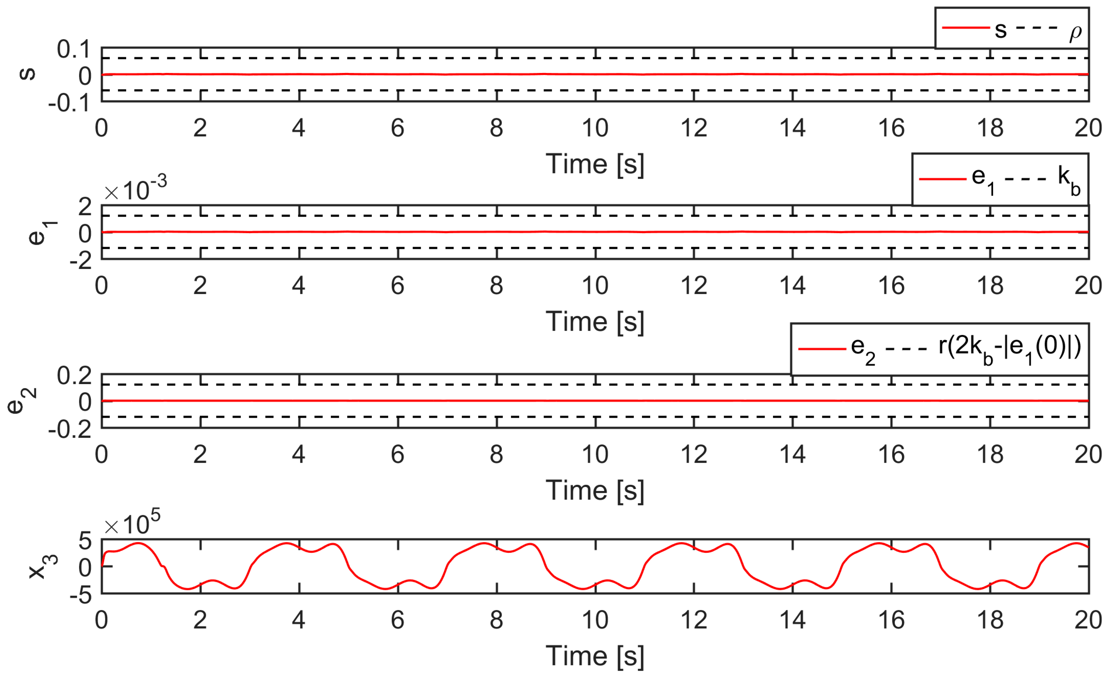
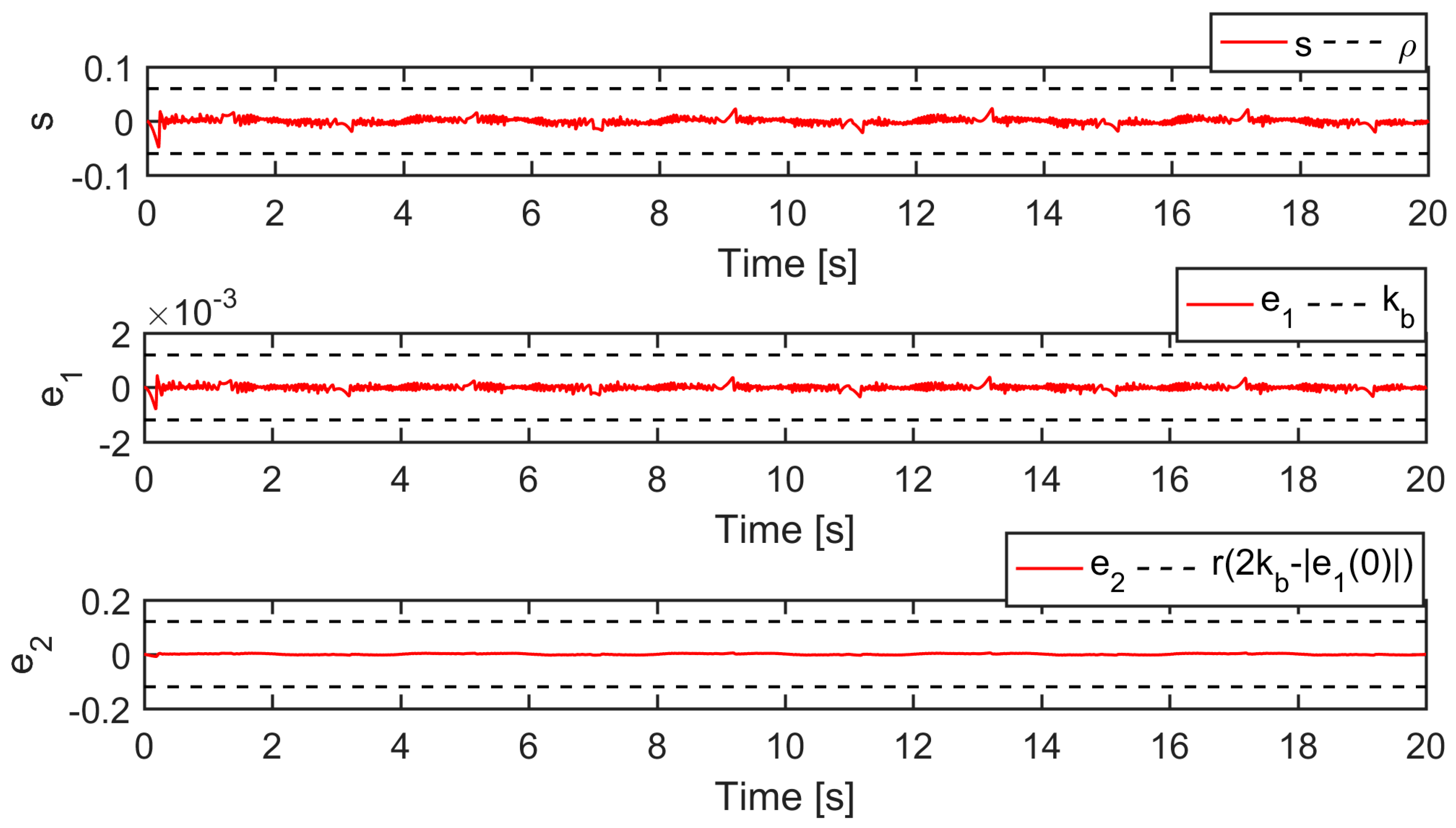
All closed-loop system signals are bounded, and the prescribed boundary of the position tracking error is never violated;

(2)

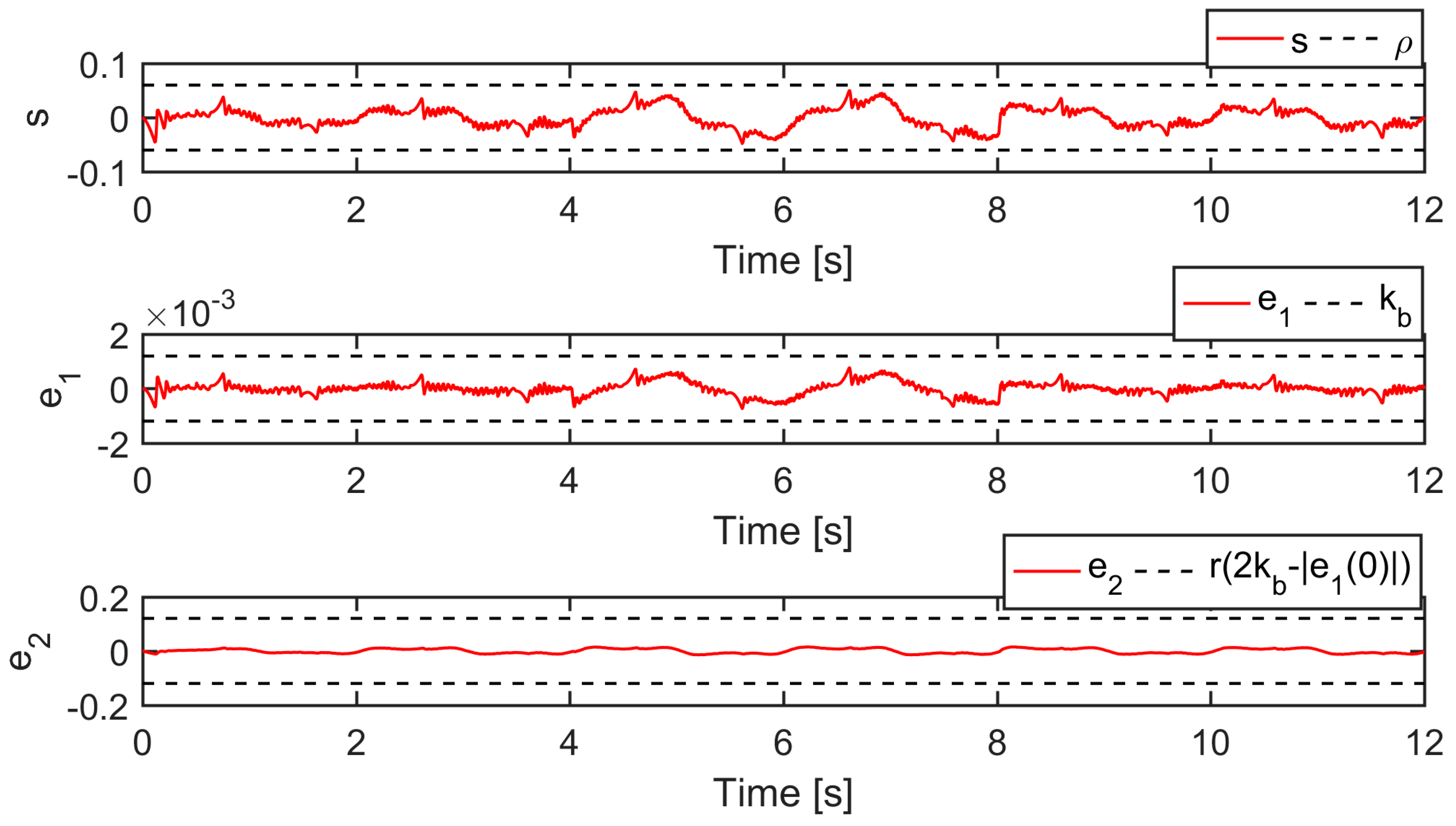
The position tracking error finally converges to a region around zero, which can be arbitrarily small by an appropriate selection of the control parameters.

Proof. 

There is a compact set ${\Omega }_v:=\left\{(s,\eta )\in (-\rho ,\rho )\times {ℝ}^2|v(s,\eta )\le 2c\right\}$ such that:

$${\Omega }_s\times {\Omega }_{\eta }\subseteq {\Omega }_v$$

(55)

The closed-loop system (47) can be regarded as a perturbed system of its reduced system and boundary layer system. The reduced and boundary layer systems have been proven to be asymptotically stable. However, the perturbation terms $f(t,s,\eta ,\epsilon )-f(t,s,0,0)$ and $g(t,s,\eta ,\epsilon )-g(t,s,\eta ,0)$ may cause the closed-loop system to become unstable.

To investigate the closed-loop system’s stability, we start with verifying the boundedness of ${\dot{\overline{\lambda }}}_1$ on Ω_v. It can be obtained from (32) and (45) that:

$${\overline{\lambda }}_1=-\frac{k_1}{a_1}s-\frac{{\widehat{d}}_1}{a_1}+\frac{{\ddot{y}}_d}{a_1}-\frac{r}{a_1}{e}_2-\frac{s}{4a_1\left({\rho }^2-s^2\right)}\left(a_1^2+1\right)$$

(56)

Then, the time derivative of ${\overline{\lambda }}_1$ is given by:

$${\dot{\overline{\lambda }}}_1=\frac{\partial {\overline{x}}_3}{\partial s}\dot{s}+\frac{\partial {\overline{x}}_3}{\partial e_2}{\dot{e}}_2+\frac{\partial {\overline{x}}_3}{\partial {\widehat{d}}_1}{\dot{\widehat{d}}}_1+\frac{\partial {\overline{x}}_3}{\partial {\ddot{y}}_d}{\stackrel{⃛}{y}}_d$$

(57)

where:

$$\frac{\partial {\overline{x}}_3}{\partial s}=-\frac{k_1}{a_1}-\frac{1}{4a_1}\frac{{\rho }^2+s^2}{{({\rho }^2-s^2)}^2}\left(a_1^2+1\right), \frac{\partial {\overline{x}}_3}{\partial e_2}=-\frac{r}{a_1}, \frac{\partial {\overline{x}}_3}{\partial {\widehat{d}}_1}=-\frac{1}{a_1}, \frac{\partial {\overline{x}}_3}{\partial {\ddot{y}}_d}=\frac{1}{a_1}$$

(58)

From (17)–(18), we obtain:

$${\dot{\widehat{d}}}_1=l_1{\eta }_2$$

(59)

Combing (47) and (59), and ${\dot{e}}_2=\dot{s}-r{e}_2$, it can be inferred that there is a continuous function M such that:

$$\left|{\dot{\overline{\lambda }}}_1\right|\le M(s,e_2,\eta ,{\stackrel{⃛}{y}}_d)$$

(60)

It is known from Lemma 1 that for all $s\in {\Omega }_s\subseteq (-\rho ,\rho )$, e₂ is bounded. It follows from Assumption 1 that ${\stackrel{⃛}{y}}_d$ is bounded. Therefore, the continuous function M has a maximum value on Ω_v. Then, it can be easily deduced that there is a positive constant φ such that the perturbation term satisfies:

$${‖g(t,s,\eta ,\epsilon )-g(t,s,\eta ,0)‖}_2\le \epsilon \phi$$

(61)

Now, differentiating (54) along the solution of (47), we have:

$$\begin{array}{c}\dot{v}=\frac{\partial V}{\partial s}f(t,s,0,0)+\frac{\partial V}{\partial s}\left[f(t,s,\eta ,\epsilon )-f(t,s,0,0)\right]+\frac{1}{\epsilon }\frac{\partial W}{\partial \eta }g(t,s,\eta ,0)\\ \hspace{1em}+\frac{1}{\epsilon }\frac{\partial W}{\partial \eta }\left[g(t,s,\eta ,\epsilon )-g(t,s,\eta ,0)\right]\\ \le -k_1\frac{s^2}{{\rho }^2-s^2}-\frac{s^2}{4{\left({\rho }^2-s^2\right)}^2}\left(a_1^2+1\right)+\frac{a_{1}s{\eta }_1}{{\rho }^2-s^2}+\frac{s{\eta }_2}{{\rho }^2-s^2}\\ \hspace{1em}-\frac{1}{\epsilon }\left(1-{‖P_{\eta }‖}_2\right){‖\eta ‖}_2^2+\phi {‖P_{\eta }‖}_2{‖\eta ‖}_2\end{array}$$

(62)

Applying Young’s inequality to $\frac{a_{1}s{\eta }_1}{{\rho }^2-s^2}$,$\frac{s{\eta }_2}{{\rho }^2-s^2}$ and $\phi {‖P_{\eta }‖}_2{‖\eta ‖}_2$, we have:

$$\begin{array}{c} \frac{a_{1}s{\eta }_1}{{\rho }^2-s^2}\le \frac{a_1^2}{4}\frac{s^2}{{\left({\rho }^2-s^2\right)}^2}+{\eta }_1^2\\ \frac{s{\eta }_2}{{\rho }^2-s^2}\le \frac{1}{4}\frac{s^2}{{\left({\rho }^2-s^2\right)}^2}+{\eta }_2^2\\ \phi {‖P_{\eta }‖}_2{‖\eta ‖}_2\le \frac{1}{4}{‖P_{\eta }‖}_2^2{‖\eta ‖}_2^2+{\phi }^2 \end{array}$$

(63)

Therefore, (62) becomes:

$$\dot{v}\le -k_1\frac{s^2}{{\rho }^2-s^2}-\frac{1}{\epsilon }\left(1-{‖P_{\eta }‖}_2-\frac{\epsilon }{4}{‖P_{\eta }‖}_2^2-\epsilon \right){‖\eta ‖}_2^2+{\phi }^2$$

(64)

To proceed with the analysis, we introduce the following lemma:

Lemma 2 [44]: 

For any given positive constant ρ, the following inequality holds for all $\left|s\right|<\rho$:

$$\log \frac{{\rho }^2}{{\rho }^2-s^2}<\frac{s^2}{{\rho }^2-s^2}$$

(65)

Applying Lemma 2 to (64) and combining the inequality $W(\eta )\le \frac{1}{2}{‖P_{\eta }‖}_2{‖\eta ‖}_2^2$, we have:

$$\dot{v}<-2k_{1}V-\frac{2}{\epsilon {‖P_{\eta }‖}_2}\left(1-{‖P_{\eta }‖}_2-\frac{\epsilon }{4}{‖P_{\eta }‖}_2^2-\epsilon \right)W+{\phi }^2\le -\sigma v+Q$$

(66)

where:

$$\sigma =2\min \left\{k_1,\frac{1}{\epsilon {‖P_{\eta }‖}_2}\left(1-{‖P_{\eta }‖}_2-\frac{\epsilon }{4}{‖P_{\eta }‖}_2^2-\epsilon \right)\right\}, Q={\phi }^2$$

(67)

(1)

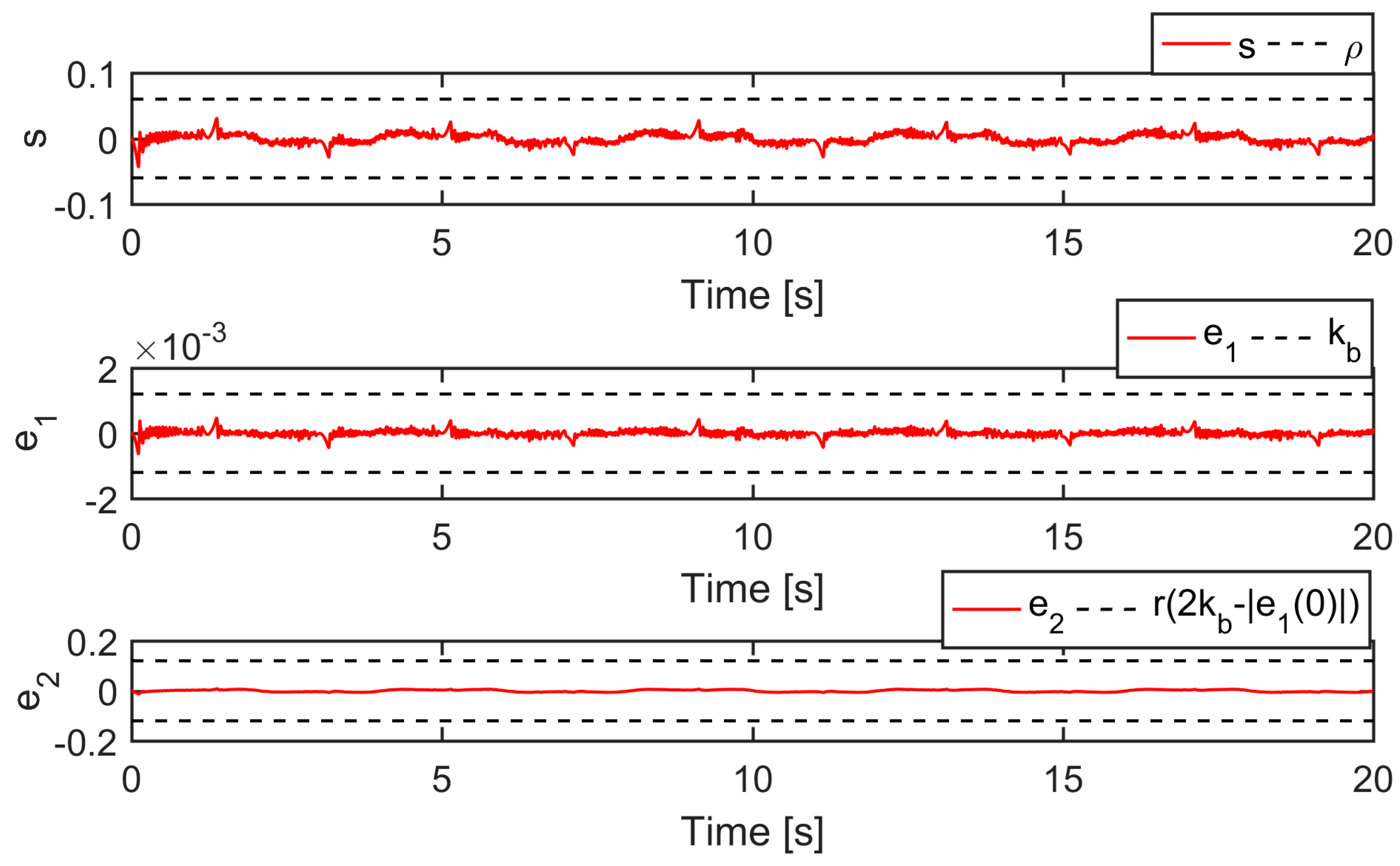
Choose k₁, k₂, h₁, and h₂ such that $Q/\sigma \le 2c$, and then we have $\dot{v}<0$ on $v(t)=2c$,$\forall t\ge 0$, which means that Ω_v is a positive invariant set. Therefore, any trajectories starting from ${\Omega }_s\times {\Omega }_{\eta }$ will remain within Ω_v. Since $v(s,\eta )$ is bounded, its components V(s) and W(η) are also bounded, and it can be concluded that η is bounded and $\left|s(t)\right|<\rho$, $\forall t\ge 0$. It follows from Lemma 1 that e₁ and e₂ are bounded by k_b and r(2k_b − |e₁(0)|), which means that the position tracking error constraint is satisfied. According to Assumptions 1–2, it can be easily inferred from (17) and (35) that x₁, x₂, ${\widehat{d}}_1$, and ${\widehat{d}}_2$ are bounded. Thus, it can be concluded from (45) that u_s is also bounded. Consequently, the boundedness of ${\overline{\lambda }}_1$ is guaranteed from (32), and $x_3={\overline{\lambda }}_1+{\eta }_1$ is also bounded. Additionally, it is known from (46) that u_f is bounded. Finally, the boundedness of u = u_s + u_f is verified.

Therefore, all closed-loop system signals are bounded, and the prescribed boundary of the position tracking error is never violated.

(2)

It follows from (66) that:

$$\dot{v}<-(1-\theta )\sigma v$$

(68)

$\forall v(t)\ge Q/\theta \sigma$, where $\theta \in (0,1)$. It follows from Theorem 4.18 in [45] that there is a time constant T such that $v(t)\le Q/\theta \sigma$, $\forall t\ge T$. Due to the fact that $\frac{1}{2}\log \frac{{\rho }^2}{{\rho }^2-s^2}\le v$, we have:

$$\left|s(t)\right|\le \rho \sqrt{1-e^{-2Q/\theta \sigma }}$$

(69)

$\forall t\ge T$. The solution ${\dot{e}}_1=-r{e}_1+s$ over the time interval [T, t] is:

$$e_1(t)=e^{-r(t-T)}{e}_1(T)+{\displaystyle {\int }_T^t{e}^{-r(t-\gamma )}}s(\gamma )d\gamma$$

(70)

Therefore:

$$\begin{array}{c}\left|e_1(t)\right|\le \left|e_1(T)\right|e^{-r(t-T)}+{\displaystyle {\int }_T^t{e}^{-r(t-\gamma )}}\left|s(\gamma )\right|d\gamma \\ \le k_b{e}^{-r(t-T)}+\frac{\rho }{r}\sqrt{1-e^{-2Q/\theta \sigma }}\end{array}$$

(71)

It means that e₁(t) finally converges to a compact set:

$${\Omega }_e:=\left\{e_1\in ℝ|\left|e_1(t)\right|\le \frac{\rho }{r}\sqrt{1-e^{-2Q/\theta \sigma }}\right\}$$

(72)

which can be arbitrarily small by an appropriate selection of the control parameters k₁, k₂, h₁, and h₂ such that σ is sufficiently large. □

Remark 5: 

It is inferred from the stability analysis that the slow control law u_s and the fast control law u_f are designed to ensure the asymptotic stability of the reduced system and the boundary layer system, respectively. Considering that the perturbation terms may cause the closed-loop system to be unstable, some restrictive conditions are imposed on the control parameters to ensure the uniformly ultimate boundedness of the closed-loop system. Meanwhile, the position tracking error constraint of the original PHA is reserved, and a satisfactory final tracking accuracy can be achieved.

Remark 6: 

It can be inferred from (42) and (72) that the transient performance and the final tracking accuracy of the position tracking error can be improved by either increasing r or decreasing ρ. Increasing σ is an alternative approach to improve the final tracking accuracy. According to (67), σ can be tuned to be large by increasing k_i (i = 1,2) or decreasing h_i (i = 1,2).

5. Simulation and Experimental Validation

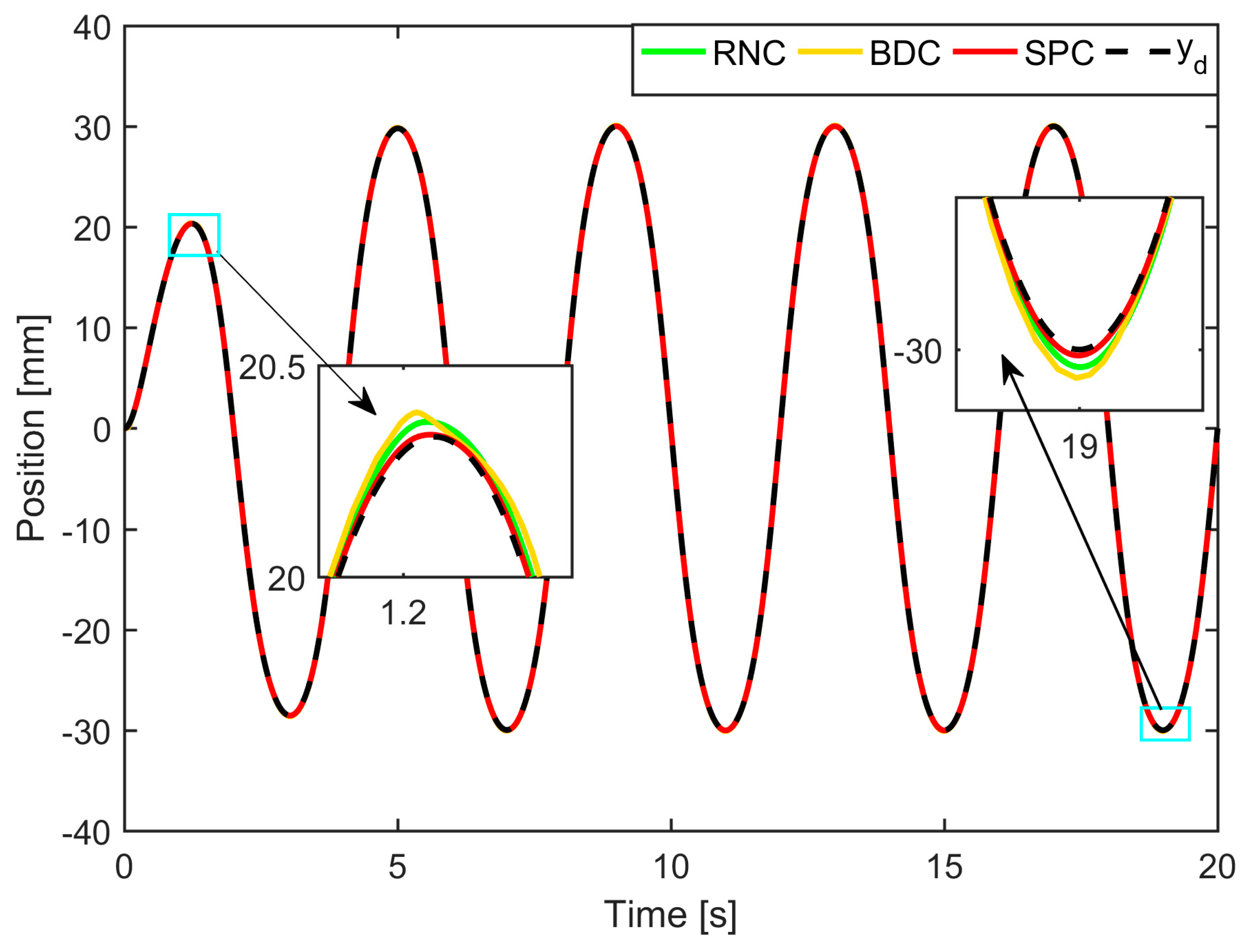
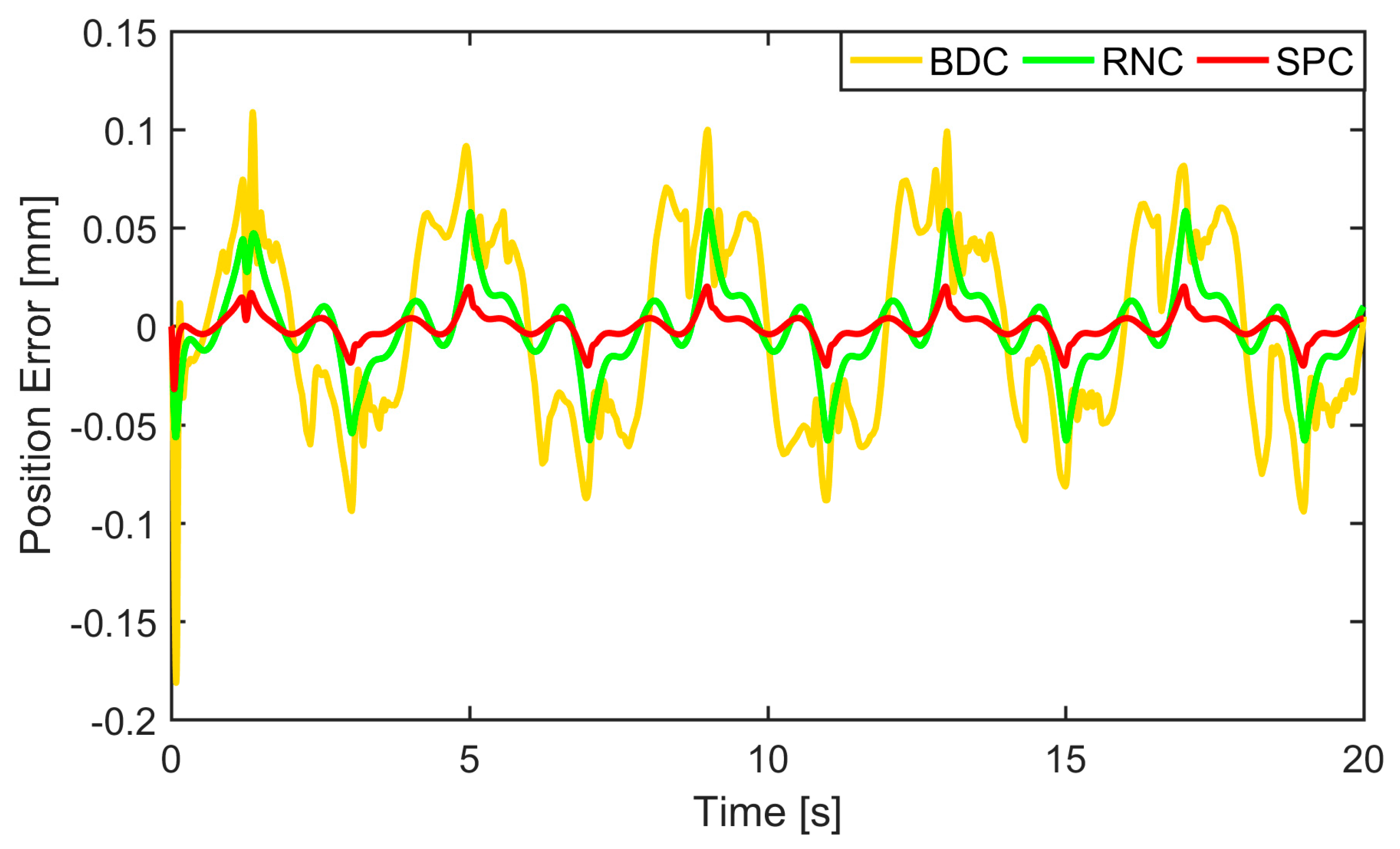
5.1. Numerical Simulation

A simulation was performed in MATLAB/Simulink to confirm the efficacy of the proposed control scheme. Referring to [46], the nominal hydraulic system parameters were selected as m = 8 kg, A = 6.4 × 10⁻⁴ m², D = 6 × 10⁻⁶ m³/rev, K_m = 4.17 rev/(sV), V₀₁ = 4.7 × 10⁻⁴ m³, V₀₂ = 5.1 × 10⁻⁴ m³, β_e = 10⁹ Pa, and C_t = 5 × 10⁻¹³ m³/(sPa). The parameters b₁, b₂, and b₃ used in the controller design were assumed to be 85%, 80%, and 70% of their nominal values, respectively. The parameters of the smooth nonlinear friction F_f in (14) were selected as γ₁ = 50, γ₂ = 150, γ₃ = 30, γ₄ = 200, γ₅ = 100, and γ₆ = 300. The external disturbance F_d was given by:

$$F_d=50\tanh (500x_2)\sin (2\pi t)$$

(73)

The reference was given as y_d(t) = 30 arctan(sin(πt/2))(1 − e^-t)/0.7854 mm. It is a sinusoidal-like trajectory with the amplitude of the actuator moving forward and backward at 30 mm, thus it can be used to test the control performance of the two directions of movement of the actuator and the pump. The prescribed bound k_b = 1.2 mm.

To demonstrate the efficacy of the proposed approach, three comparable controllers are constructed as follows:

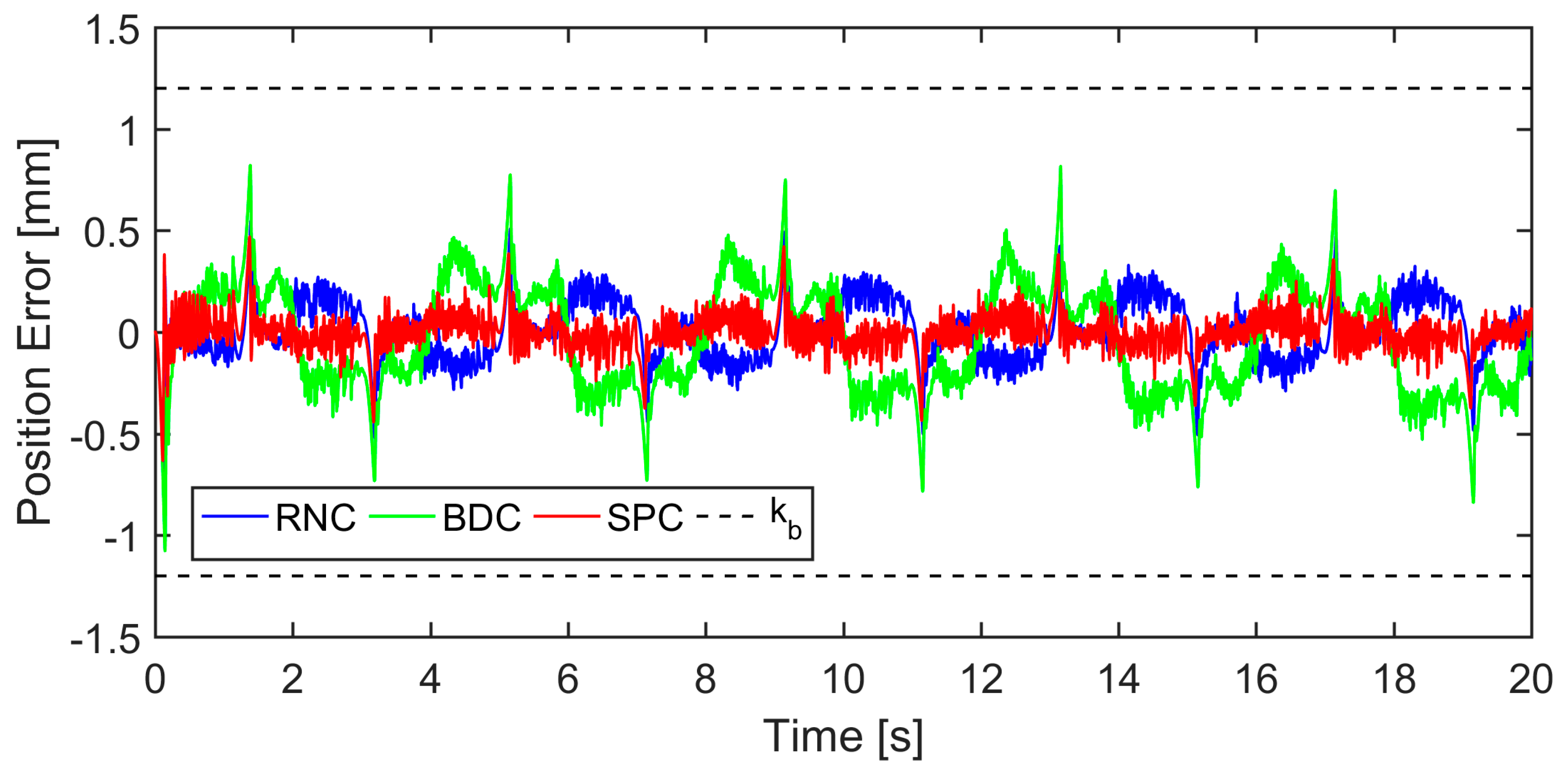
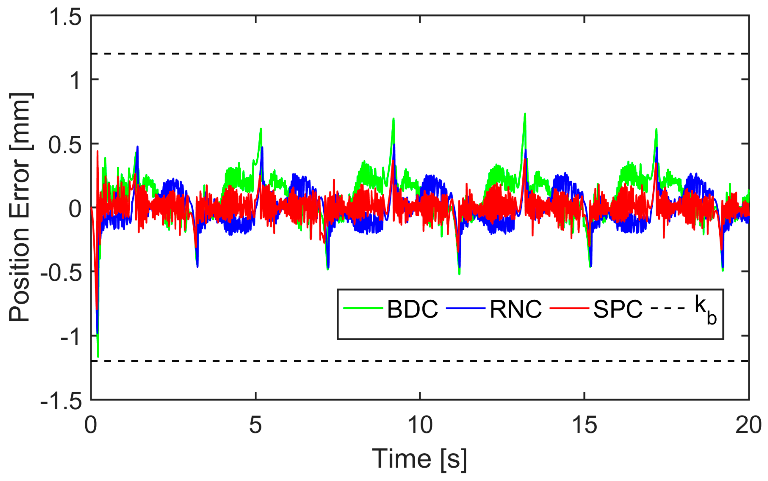
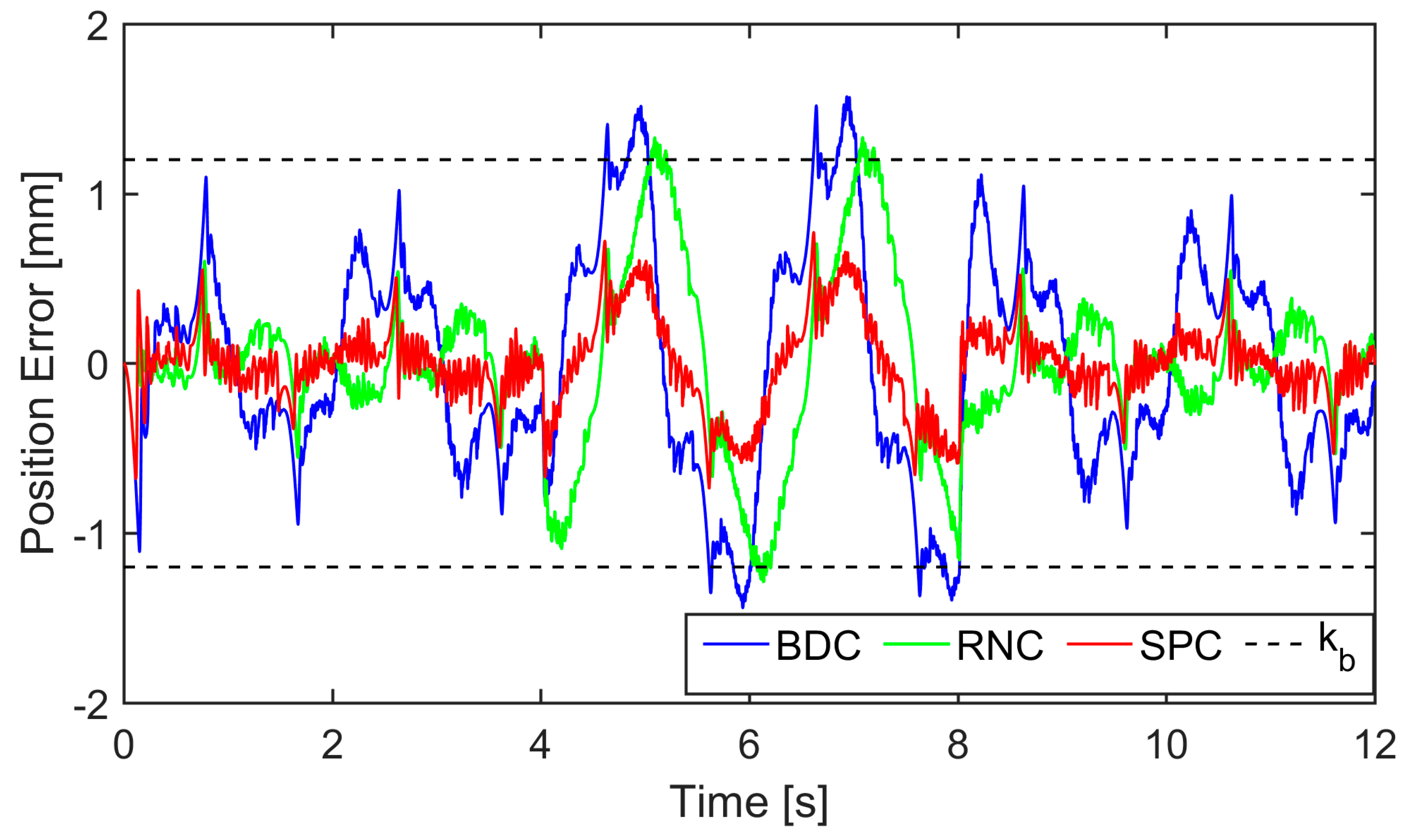
(1)

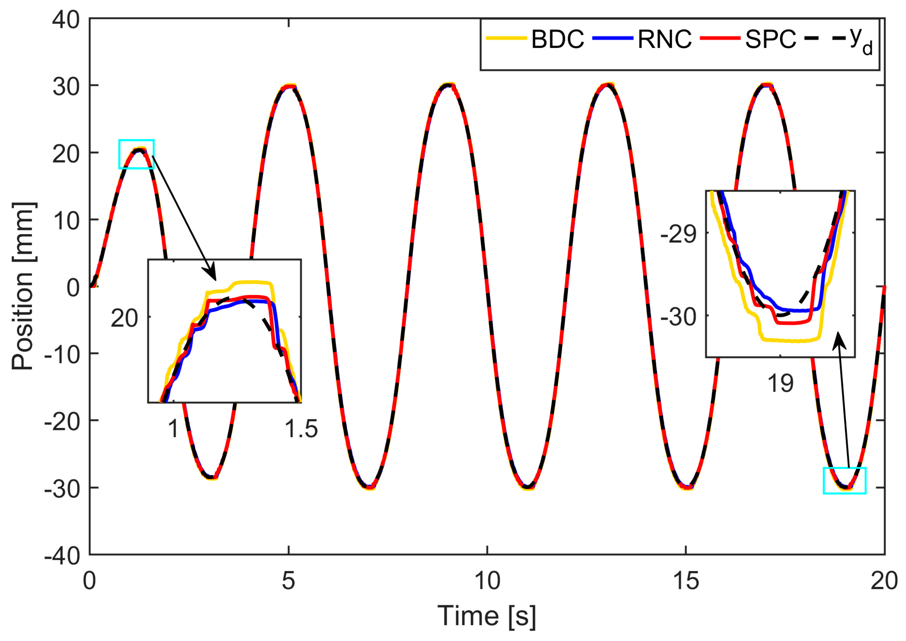
SPC: This is the proposed singular perturbation theory-based composite controller with the sliding surface-like error variable. The controller parameters of SPC are chosen as k₁ = 10⁵, k₂ = 5 × 10⁻¹⁰, h₁ = 5 × 10⁵, h₂ = 10⁶, ρ = 0.06, and r = 50.

(2)

RNC: This is a reduce-order model-based nonlinear controller proposed in [23]. It is constructed as:

$$u=\frac{b_3}{a_1{b}_1}\left(-L_1{e}_1-L_2{e}_2+\frac{a_1{b}_2}{b_3}{x}_2+{\ddot{y}}_d-{\widehat{d}}_1-\frac{a_1}{b_3}{\widehat{d}}_2\right)$$

(74)

The feedback gains are selected as L₁ = 2 × 10⁶ and L₂ = 1.5 × 10⁵. The uncertainty estimates ${\widehat{d}}_1$ and ${\widehat{d}}_2$ are obtained from (16). All other parameters are chosen the same as SPC to form a fair comparison.

(3)

BDC: This is a backstepping controller with dynamic surface control. The structure and control parameters of BDC were shown as follows:

$${\alpha }_1=-{\gamma }_1{z}_1+{\dot{y}}_d$$

(75)

$${\alpha }_2=\frac{1}{a_1}\left(-{\gamma }_2{z}_2-z_1-{\widehat{d}}_1+{\dot{\alpha }}_{1d}\right)$$

(76)

$$u=\frac{1}{{\beta }_e{b}_1}\left(-{\gamma }_3{z}_3-a_1{z}_2+b_2{\beta }_e{x}_2+b_3{\beta }_e{x}_3-{\beta }_e{\widehat{d}}_2+{\dot{\alpha }}_{2d}\right)$$

(77)

$${\tau }_1{\dot{\alpha }}_{1d}+{\alpha }_{1d}={\alpha }_1,\hspace{1em}{\alpha }_{1d}(0)={\alpha }_1(0)$$

(78)

$${\tau }_2{\dot{\alpha }}_{2d}+{\alpha }_{2d}={\alpha }_2,\hspace{1em}{\alpha }_{2d}(0)={\alpha }_2(0)$$

(79)

where $z_1=y-y_d, z_2=x_2-{\alpha }_{1d}, z_3=x_3-{\alpha }_{2d}$ and ${\widehat{d}}_1$ and ${\widehat{d}}_2$ were obtained from (16). The control parameters were selected as γ₁ = 50, γ₂ = 1000, γ₃ = 30, and τ₁ = τ₂ = 0.015. All other parameters are chosen the same as the proposed approach to form a fair comparison.

The simulation results displayed in Figure 3 and Figure 4 illustrate that all controllers retained their position tracking errors within the prescribed bound, and SPC performed better than RNC and BDC, which illustrates the effectiveness of the proposed sliding surface-like error variable s in output tracking error constraint. The boundedness of s, e₁, and e₂ is exhibited in Figure 5. Consistent with Lemma 1, it was constrained by ρ, k_b, and r(2k_b − |e₁(0)|), respectively. Therefore, the position tracking error constraint was achieved. Moreover, it is inferred from (35) that x₁ and x₂ are bounded. The boundedness of x₃ is also shown in Figure 5. Additionally, the profiles of the uncertainty estimation are displayed in Figure 6. As seen, the estimates obtained by the DOBs in (16) tracked their actual values well. The control signal is shown in Figure 7, which was continuous and bounded.

Remark 7: 

A stringent guideline of control parameter selection has been given in Theorem 3. It implies that for any given initial condition, there always are sufficiently large control parameters k₁, k₂, l₁, and l₂ such that the desired control performance can be achieved. However, the guideline is too complex to follow in practical applications. More seriously, as commented in [47], the parameter values calculated from stability analysis may be unrealistic in practice since they normally take into account the bounding information of uncertainties and system parameters. In this paper, similar to the approach in [48], we start with small feedback gains and gradually increase them until satisfactory control performance is achieved. The observer gains are then tuned up to estimate the uncertainties, which also helps to improve the control accuracy. However, we should note that overly large control parameters can cause oscillations, and thus the tuning process should be careful.

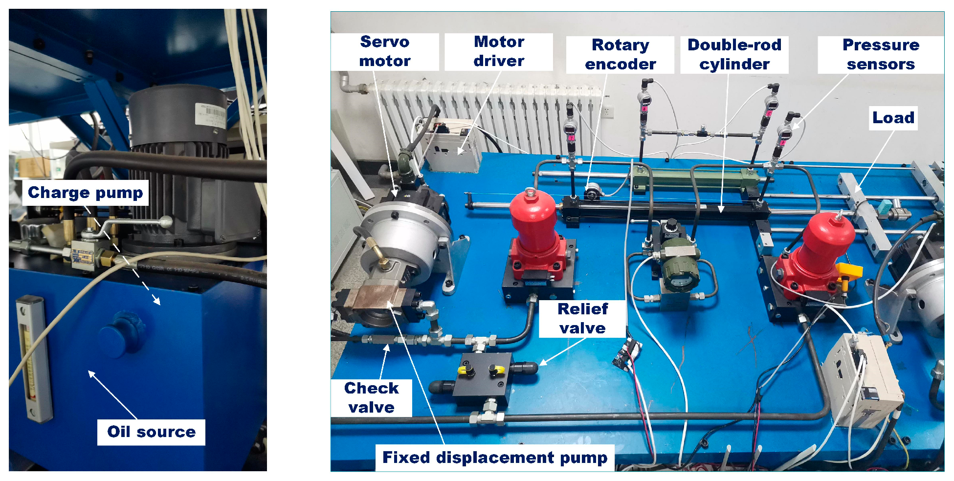
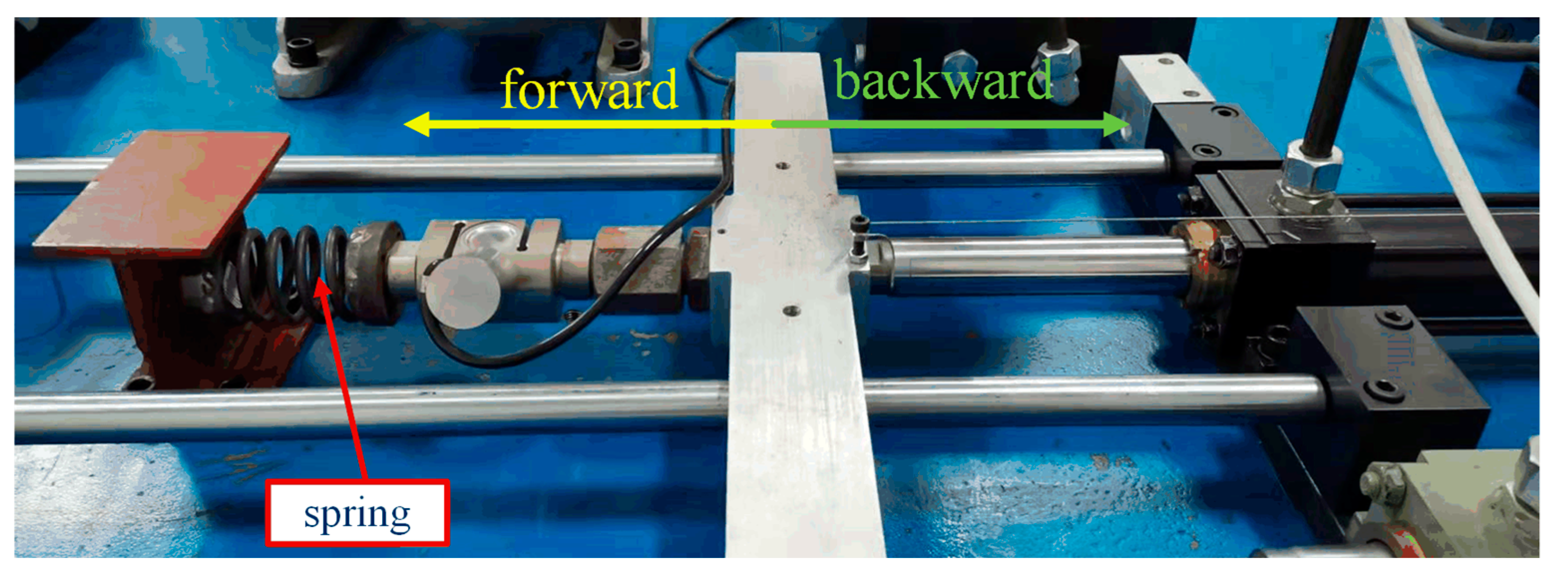
5.2. Experimental Setup

An actual PHA, shown in Figure 8, is set up to test the practicality of the proposed control scheme. The PHA includes a Parker double-rod cylinder, a fixed displacement pump (Rexroth A10FZG006/10W), and a servo motor (Yaskawa SGM7G-30AFC61). A rotary encoder (Kübler 8.5000.8132.5000) and two pressure sensors (HYDAC EDS 3448-5-0100-Y00) are installed to measure the required position and pressure signals. The velocity signal is obtained by applying a backward difference algorithm to the position signal. Two second-order Butterworth filters with a cutoff frequency of 20 Hz are adopted to avoid measurement noise in the velocity and pressure signals [49]. The measured signals are then sampled with a sampling period T_s = 1 ms and transmitted to a host PC via a data acquisition module, Quanser Q8-usb. Control algorithms are constructed and executed in MATLAB/Simulink, which communicates with Quanser Q8-usb via the embedded QUARC to transmit the control data to the DC motor driver.

5.3. Experimental Results

To investigate the superiority of the proposed scheme, RNC and BDC were employed for comparison. To quantitatively evaluate their performances, we introduce three performance indices as follows:

(1)

The maximum absolute error:

$$\mathrm{MAX}={\max }_{i=1, \dots , N}\left\{\left|e_1\left(i\right)\right|\right\}$$

(80)

(2)

The integral of the squared errors:

$$\mathrm{ISE}={\displaystyle \sum _{i=1}^N{\left[e_1(i)\right]}^2}\cdot T_s$$

(81)

(3)

The integral of time multiplied by the absolute errors:

$$\mathrm{ITAE}={\displaystyle \sum _{i=1}^N\left|e_1(i)\right|}\cdot i{T}_s$$

(82)

where N represents the number of the sampled data.

Case 1: A low-frequency smooth reference trajectory y_d(t) = 30 arctan(sin(πt/2))(1 − e^−t)/0.7854 mm was used for the controllers, and the prescribed bound k_b = 1.2 mm. The experimental results are depicted in Figure 9 and Figure 10 and

Table 1. Performance indices of the compared controllers during 16–20 s.

Indices	MAX (mm∙s)	ISE (mm2∙s)	ITAE (m∙s)
SPC RNC	0.374 0.484	0.029 0.086	0.469 0.896
BDC	0.839	0.322	2.189

. It is obvious that all the controllers constrained their position tracking errors within the prescribed bound. Nevertheless, SPC performed better than RNC and BDC with its position tracking error shown in Figure 10, which was farther away from the prescribed bound. The reason is because the term $s\left(1+a_1^2\right)/4\left({\rho }^2-s^2\right)$ in (45) will grow rapidly to provide a strong enough control action to prevent the position tracking error from approaching its bound. The profiles of s, e₁, and e₂ of SPC are plotted in Figure 11. They were, respectively, bounded by ρ, k_b, and r(2k_b-|e₁(0)|), which verifies the efficacy of the designed sliding surface-like error variable s in ensuring that e₁ and e₂ are constrained by the known bounds. In addition, the boundedness of the uncertainty estimation and the control signal are verified in Figure 12 and Figure 13.

Case 2: To test the robustness of the compared controllers, a spring, shown in Figure 14, was installed to strengthen the mismatched uncertainties. The reference was chosen as y_d(t) = 15 arctan(sin(πt/2))(1 − e^−t)/0.7854 mm, and the spring was pre-compressed by 18 mm. This setting makes the spring compression vary from 3 mm to 33 mm when the actuator moves forward and backward. It means that the additive spring force was nonvanishing during the operation process. The tracking performances are displayed in Figure 15 and

Table 2. Performance indices of the compared controllers during 16–20 s.

Indices	MAX (mm∙s)	ISE (mm2∙s)	ITAE (m∙s)
SPC	0.344	0.027	0.460
RNC	0.470	0.075	0.862
BDC	0.612	0.140	0.859

. As seen, all controllers constrained their position tracking errors within the prescribed bound under the strengthened mismatched uncertainties. Nevertheless, SPC performed better than RNC and BDC in both the transient and steady-state periods, which demonstrated the superiority of the proposed control strategy. s, e₁, and e₂ of SPC were plotted in Figure 16 to confirm the robustness of the proposed control approach in state constraint under external disturbance. In addition, it can be inferred from force analysis that the friction and spring force have the same sign when the actuator moves forward, while the spring force counteracts partial friction when the actuator moves backward. It renders the lumped mismatched uncertainty asymmetrical. The estimate of d₁, shown in Figure 17, illustrates that the incorporated DOB reproduced the asymmetry of the uncertainties.

Case 3: To test the robustness of the controllers against the matched uncertainties, similar to [48], a disturbance was selected as $u_d=10{\dot{y}}_d$V and exerted on the control input during 4 s and 8 s. In this period, u* = u − u_d was actually applied to control the PHA. The reference was chosen as y_d(t) = 15 arctan(sin(πt))(1 − e^−t)/0.7854 mm. The position tracking errors of the compared controllers are plotted in Figure 18, and their performance indices during 4 s and 8 s are collected in

Table 3. Performance indices of the compared controllers during 4 s and 8 s.

Indices	MAX (mm∙s)	ISE (mm2∙s)	ITAE (m∙s)
SPC RNC	0.772 1.331	0.537 2.428	2.646 5.613
BDC	1.571	3.354	6.961

. In this case, SPC successfully retained its position tracking error within the prescribed bound while RNC and BDC failed, which illustrates the efficacy of the proposed sliding surface-like error variable in state constraint. s, e₁, and e₂ of SPC were drawn in Figure 19 to confirm that they were constrained by the bounds given in Lemma 1. In addition, it can be seen in Figure 20 that the DOB captured the dramatic changes in the estimate of d₂ when the input disturbance was exerted.

6. Conclusions

In this article, we present a singular perturbation theory-based composite control approach for a PHA with position tracking error constraint. The PHA can be separated into the second-order slow mechanical and first-order fast hydraulic subsystems from the two-time scale perspective. Slow and fast control laws are decoupled to work as the inputs of the corresponding subsystems. To facilitate position tracking error constraint control without the backstepping technique, a sliding surface-like error variable is proposed to transform the second-order mechanical subsystem into a first-order error subsystem, where a BLF-based slow control law can be easily designed without any intermediate virtual control law. Two DOBs are incorporated in the controller design to provide estimates of the uncertainties. The remaining fast control law is designed to make the first-order hydraulic subsystem asymptotically converge to its equilibrium point related to the slow control law. The theoretical analysis gives rigorous proof of the closed-loop system’s stability. Simulations and experiments are conducted to test the efficacy and practicability of the developed control approach.

References

- Shang, Y.; Li, X.; Qian, H.; Wu, S.; Pan, Q.; Huang, L.; Jiao, Z. A Novel Electro Hydrostatic Actuator System with Energy Recovery Module for More Electric Aircraft. IEEE Trans. Ind. Electron. 2020, 67, 2991–2999. [Google Scholar] [CrossRef]
- Chen, S.-H.; Fu, L.-C. Observer-Based Backstepping Control of a 6-Dof Parallel Hydraulic Manipulator. Control Eng. Pract. 2015, 36, 100–112. [Google Scholar] [CrossRef]
- Yu, T.; Plummer, A.R.; Iravani, P.; Bhatti, J.; Zahedi, S.; Moser, D. The Design, Control, and Testing of an Integrated Electrohydrostatic Powered Ankle Prosthesis. IEEE/ASME Trans. Mechatron. 2019, 24, 1011–1022. [Google Scholar] [CrossRef]
- Imam, A.; Tolba, M.; Sepehri, N. A Comparative Study of Two Common Pump-Controlled Hydraulic Circuits for Single-Rod Actuators. Actuators 2023, 12, 193. [Google Scholar] [CrossRef]
- Alle, N.; Hiremath, S.S.; Makaram, S.; Subramaniam, K.; Talukdar, A. Review on Electro Hydrostatic Actuator for Flight Control. Int. J. Fluid Power 2016, 17, 125–145. [Google Scholar] [CrossRef]
- Ho, T.H.; Le, T.D. Development and Evaluation of Energy-Saving Electro-Hydraulic Actuator. Actuators 2021, 10, 302. [Google Scholar] [CrossRef]
- Bakhshande, F.; Bach, R.; Söffker, D. Robust Control of a Hydraulic Cylinder Using an Observer-Based Sliding Mode Control: Theoretical Development and Experimental Validation. Control Eng. Pract. 2020, 95, 104272. [Google Scholar] [CrossRef]
- Barchi, D.; Macchelli, A.; Bosi, G.; Marconi, L.; Foschi, D.; Mezzetti, M. Design of a Robust Adaptive Controller for a Hydraulic Press and Experimental Validation. IEEE Trans. Control Syst. Technol. 2021, 29, 2049–2064. [Google Scholar] [CrossRef]
- Yao, Z.; Yao, J.; Sun, W. Adaptive RISE Control of Hydraulic Systems with Multilayer Neural-Networks. IEEE Trans. Ind. Electron. 2019, 66, 8638–8647. [Google Scholar] [CrossRef]
- Chen, W.-H.; Ballance, D.J.; Gawthrop, P.J.; O’Reilly, J. A Nonlinear Disturbance Observer for Robotic Manipulators. IEEE Trans. Ind. Electron. 2000, 47, 932–938. [Google Scholar] [CrossRef]
- Han, J. From PID to Active Disturbance Rejection Control. IEEE Trans. Ind. Electron. 2009, 56, 900–906. [Google Scholar] [CrossRef]
- Liu, K.; Wang, R. Antisaturation Command Filtered Backstepping Control-Based Disturbance Rejection for a Quadarotor UAV. IEEE Trans. Circuits Syst. II 2021, 68, 3577–3581. [Google Scholar] [CrossRef]
- Liu, K.; Wang, R.; Zheng, S.; Dong, S.; Sun, G. Fixed-Time Disturbance Observer-Based Robust Fault-Tolerant Tracking Control for Uncertain Quadrotor UAV Subject to Input Delay. Nonlinear Dyn. 2022, 107, 2363–2390. [Google Scholar] [CrossRef]
- Nguyen, M.H.; Ahn, K.K. Output Feedback Robust Tracking Control for a Variable-Speed Pump-Controlled Hydraulic System Subject to Mismatched Uncertainties. Mathematics 2023, 11, 1783. [Google Scholar] [CrossRef]
- Liu, K.; Wang, X.; Wang, R.; Sun, G.; Wang, X. Antisaturation Finite-Time Attitude Tracking Control Based Observer for a Quadrotor. IEEE Trans. Circuits Syst. II 2021, 68, 2047–2051. [Google Scholar] [CrossRef]
- Nguyen, M.H.; Dao, H.V.; Ahn, K.K. Extended Sliding Mode Observer-based High-accuracy Motion Control for Uncertain Electro-hydraulic Systems. Int. J. Robust Nonlinear 2023, 33, 1351–1370. [Google Scholar] [CrossRef]
- Tee, K.P.; Ge, S.S.; Tay, E.H. Barrier Lyapunov Functions for the Control of Output-Constrained Nonlinear Systems. Automatica 2009, 45, 918–927. [Google Scholar] [CrossRef]
- Guo, Q.; Zhang, Y.; Celler, B.G.; Su, S.W. State-Constrained Control of Single-Rod Electrohydraulic Actuator with Parametric Uncertainty and Load Disturbance. IEEE Trans. Control Syst. Technol. 2018, 26, 2242–2249. [Google Scholar] [CrossRef]
- Xu, Z.; Qi, G.; Liu, Q.; Yao, J. ESO-Based Adaptive Full State Constraint Control of Uncertain Systems and Its Application to Hydraulic Servo Systems. Mech. Syst. Signal Process. 2022, 167, 108560. [Google Scholar] [CrossRef]
- Xu, Z.; Qi, G.; Liu, Q.; Yao, J. Output Feedback Disturbance Rejection Control for Full-State Constrained Hydraulic Systems with Guaranteed Tracking Performance. Appl. Math. Model. 2022, 111, 332–348. [Google Scholar] [CrossRef]
- Swaroop, D.; Hedrick, J.K.; Yip, P.P.; Gerdes, J.C. Dynamic Surface Control for a Class of Nonlinear Systems. IEEE Trans. Automat. Control 2000, 45, 1893–1899. [Google Scholar] [CrossRef]
- Yao, J.; Deng, W.; Sun, W. Precision Motion Control for Electro-Hydraulic Servo Systems with Noise Alleviation: A Desired Compensation Adaptive Approach. IEEE/ASME Trans. Mechatron. 2017, 22, 1859–1868. [Google Scholar] [CrossRef]
- Wang, C.; Quan, L.; Zhang, S.; Meng, H.; Lan, Y. Reduced-Order Model Based Active Disturbance Rejection Control of Hydraulic Servo System with Singular Value Perturbation Theory. ISA Trans. 2017, 67, 455–465. [Google Scholar] [CrossRef]
- Kokotovic, P.V.; Khalil, H.K.; O’Reilly, J. Singular Perturbation Methods in Control: Analysis and Design; Academic Press: New York, NY, USA, 1986. [Google Scholar]
- Huang, Z.; Xu, Y.; Ren, W.; Fu, C.; Cao, R.; Kong, X.; Li, W. Design of Position Control Method for Pump-Controlled Hydraulic Presses via Adaptive Integral Robust Control. Processes 2021, 10, 14. [Google Scholar] [CrossRef]
- Ahn, K.K.; Nam, D.N.C.; Jin, M. Adaptive Backstepping Control of an Electrohydraulic Actuator. IEEE/ASME Trans. Mechatron. 2014, 19, 987–995. [Google Scholar] [CrossRef]
- Rath, J.J.; Defoort, M.; Sentouh, C.; Karimi, H.R.; Veluvolu, K.C. Output-Constrained Robust Sliding Mode Based Nonlinear Active Suspension Control. IEEE Trans. Ind. Electron. 2020, 67, 10652–10662. [Google Scholar] [CrossRef]
- Wang, Y.; Zhao, J.; Zhang, H.; Wang, H. Robust Output Feedback Control for Electro-Hydraulic Servo System with Error Constraint Based on High-Order Sliding Mode Observer. Trans. Inst. Meas. Control 2023, 45, 1703–1712. [Google Scholar] [CrossRef]
- Won, D.; Kim, W.; Shin, D.; Chung, C.C. High-Gain Disturbance Observer-Based Backstepping Control with Output Tracking Error Constraint for Electro-Hydraulic Systems. IEEE Trans. Control Syst. Technol. 2015, 23, 787–795. [Google Scholar] [CrossRef]
- Jelali, M.; Kroll, A. Hydraulic Servo-Systems; Springer: London, UK, 2003. [Google Scholar]
- Helian, B.; Chen, Z.; Yao, B.; Lyu, L.; Li, C. Accurate Motion Control of a Direct-Drive Hydraulic System with an Adaptive Nonlinear Pump Flow Compensation. IEEE/ASME Trans. Mechatron. 2021, 26, 2593–2603. [Google Scholar] [CrossRef]
- Habibi, S.; Goldenberg, A. Design of a New High-Performance Electrohydraulic Actuator. IEEE/ASME Trans. Mechatron. 2000, 5, 158–164. [Google Scholar] [CrossRef]
- Chen, Z.; Helian, B.; Zhou, Y.; Geimer, M. An Integrated Trajectory Planning and Motion Control Strategy of a Variable Rotational Speed Pump-Controlled Electro-Hydraulic Actuator. IEEE/ASME Trans. Mechatron. 2023, 28, 588–597. [Google Scholar] [CrossRef]
- Chen, G.; Liu, H.; Jia, P.; Qiu, G.; Yu, H.; Yan, G.; Ai, C.; Zhang, J. Position Output Adaptive Backstepping Control of Electro-Hydraulic Servo Closed-Pump Control System. Processes 2021, 9, 2209. [Google Scholar] [CrossRef]
- Armstrong-Hélouvry, B.; Dupont, P.; De Wit, C.C. A Survey of Models, Analysis Tools and Compensation Methods for the Control of Machines with Friction. Automatica 1994, 30, 1083–1138. [Google Scholar] [CrossRef]
- Makkar, C.; Dixon, W.E.; Sawyer, W.G.; Hu, G. A New Continuously Differentiable Friction Model for Control Systems Design. In Proceedings of the 2005 IEEE/ASME International Conference on Advanced Intelligent Mechatronics, Monterey, CA, USA, 24–28 July 2005; pp. 600–605. [Google Scholar]
- Thenozhi, S.; Sanchez, A.C.; Rodriguez-Resendiz, J. A Contraction Theory-Based Tracking Control Design with Friction Identification and Compensation. IEEE Trans. Ind. Electron. 2022, 69, 6111–6120. [Google Scholar] [CrossRef]
- Yao, J.; Deng, W.; Jiao, Z. Adaptive Control of Hydraulic Actuators with LuGre Model-Based Friction Compensation. IEEE Trans. Ind. Electron. 2015, 62, 6469–6477. [Google Scholar] [CrossRef]
- Deng, W.; Zhou, H.; Zhou, J.; Yao, J. Neural Network-Based Adaptive Asymptotic Prescribed Performance Tracking Control of Hydraulic Manipulators. IEEE Trans. Syst. Man Cybern. Syst. 2023, 53, 285–295. [Google Scholar] [CrossRef]
- Wang, S.; Yu, H.; Yu, J. Robust Adaptive Tracking Control for Servo Mechanisms with Continuous Friction Compensation. Control Eng. Pract. 2019, 87, 76–82. [Google Scholar] [CrossRef]
- Krstić, M.; Kanellakopoulos, I.; Kokotović, P.V. Nonlinear and Adaptive Control Design; Adaptive and Learning Systems for Signal Processing, Communications, and Control; Wiley: New York, NY, USA, 1995. [Google Scholar]
- Zang, W.; Chen, X.; Zhao, J. Multi-Disturbance Observers-Based Nonlinear Control Scheme for Wire Rope Tension Control of Hoisting Systems with Backstepping. Actuators 2022, 11, 321. [Google Scholar] [CrossRef]
- Ran, M.; Li, J.; Xie, L. A New Extended State Observer for Uncertain Nonlinear Systems. Automatica 2021, 131, 109772. [Google Scholar] [CrossRef]
- Ren, B.; Ge, S.S.; Tee, K.P.; Lee, T.H. Adaptive Neural Control for Output Feedback Nonlinear Systems Using a Barrier Lyapunov Function. IEEE Trans. Neural Netw. 2010, 21, 1339–1345. [Google Scholar]
- Khalil, H.K. Nonlinear Systems, 3rd ed.; Prentice Hall: Upper Saddle River, NJ, USA, 2002. [Google Scholar]
- Cai, Y.; Ren, G.; Song, J.; Sepehri, N. High Precision Position Control of Electro-Hydrostatic Actuators in the Presence of Parametric Uncertainties and Uncertain Nonlinearities. Mechatronics 2020, 68, 102363. [Google Scholar] [CrossRef]
- Sobczyk, M.R.; Gervini, V.I.; Perondi, E.A.; Cunha, M.A.B. A Continuous Version of the LuGre Friction Model Applied to the Adaptive Control of a Pneumatic Servo System. J. Frankl. Inst. 2016, 353, 3021–3039. [Google Scholar] [CrossRef]
- Gu, W.; Yao, J.; Yao, Z.; Zheng, J. Robust Adaptive Control of Hydraulic System with Input Saturation and Valve Dead-Zone. IEEE Access 2018, 6, 53521–53532. [Google Scholar] [CrossRef]
- Wang, C.; Quan, L.; Jiao, Z.; Zhang, S. Nonlinear Adaptive Control of Hydraulic System with Observing and Compensating Mismatching Uncertainties. IEEE Trans. Control Syst. Technol. 2018, 26, 927–938. [Google Scholar] [CrossRef]