


Control of an Outer Rotor Doubly Salient Permanent Magnet Generator for Fixed Pitch kW Range Wind Turbine Using Overspeed Flux Weakening Operations


 ,
, 
Abstract
1. Introduction
- − Energy conversion optimization with variable speed operations;
- − Direct coupling of turbine and generator by eliminating the gearbox.

2. Wind Turbine and OR−DSPMG Modelling
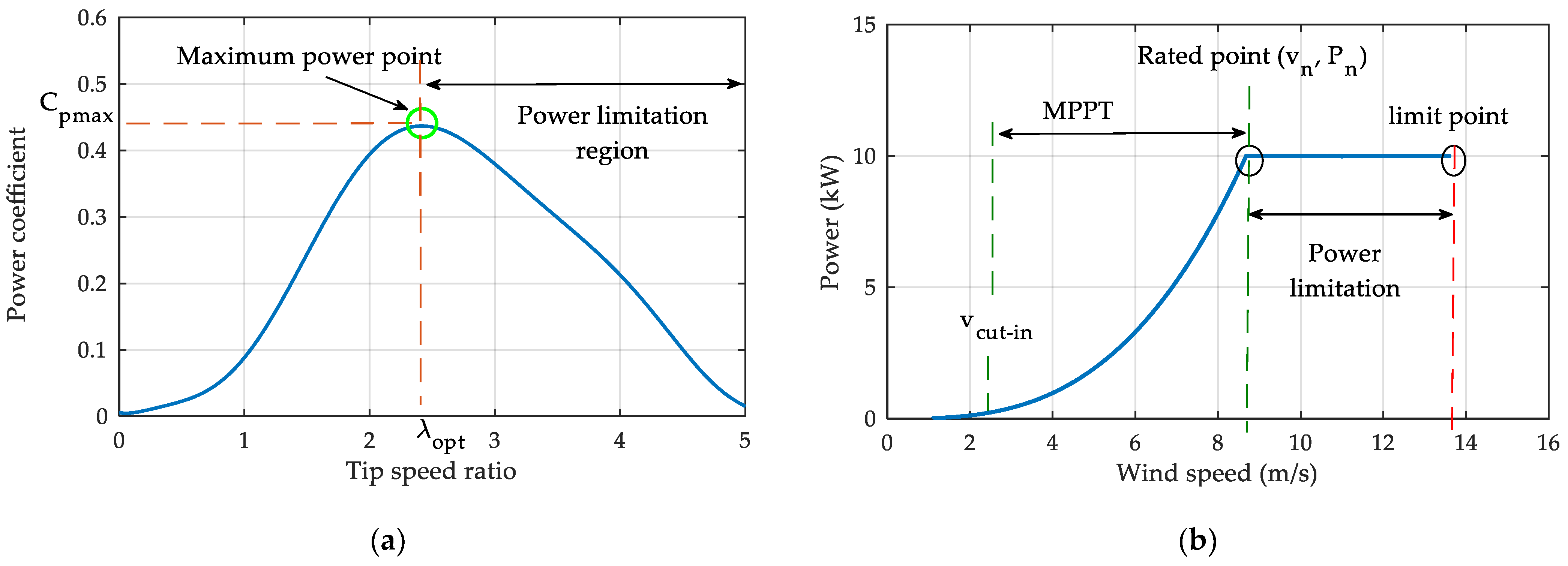
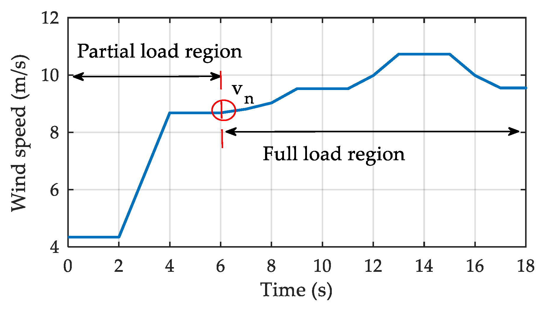
2.1. Wind Turbine Modelling

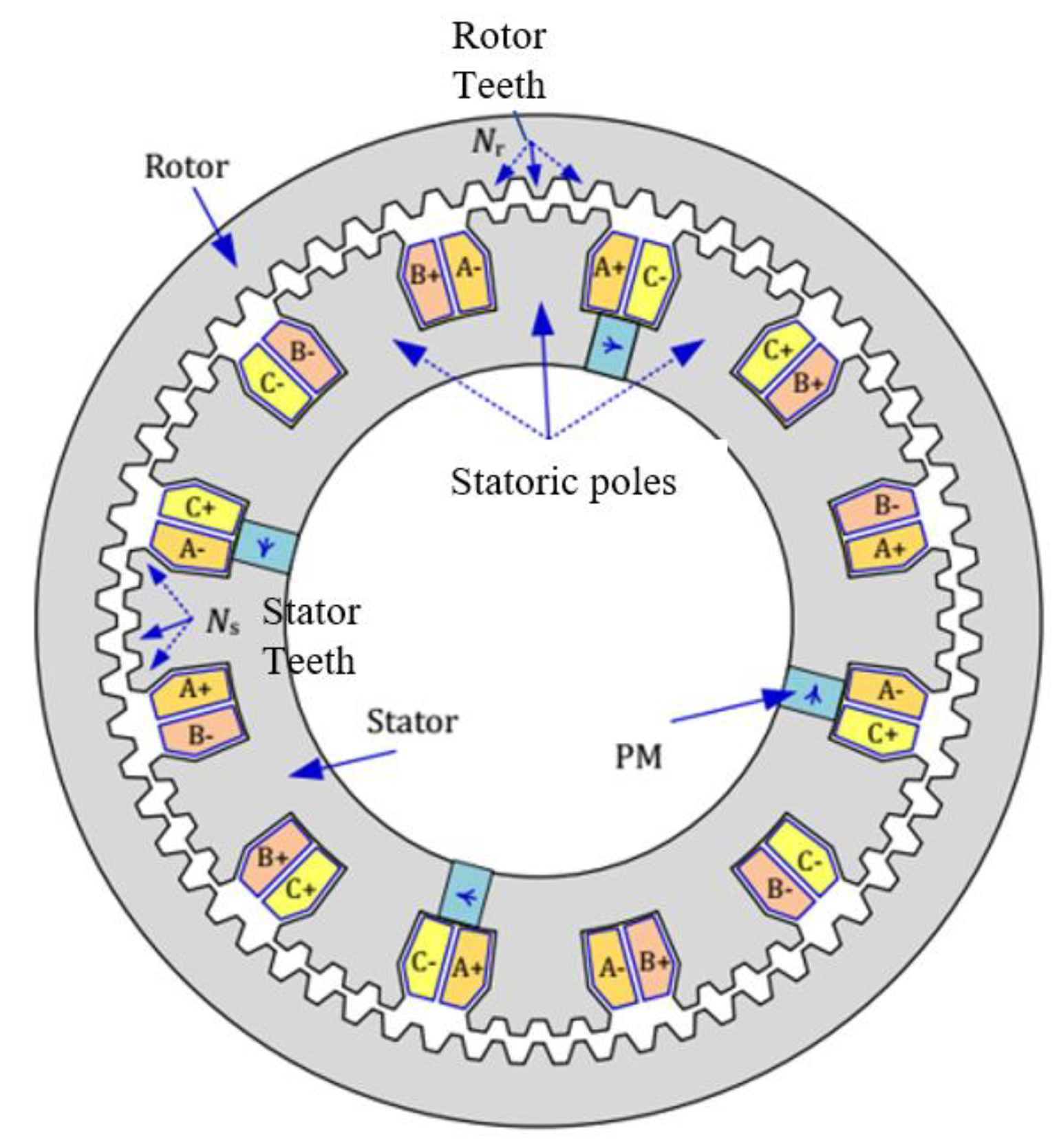
2.2. OR−DSPMG Modelling
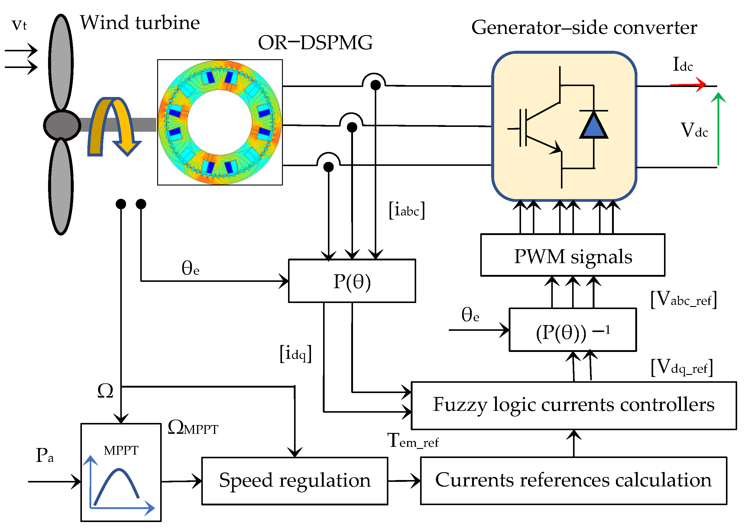
3. WECS Control
3.1. OR–DSPMSG–Side Converter Control

3.1.1. Maximum Torque Per Ampere Strategy
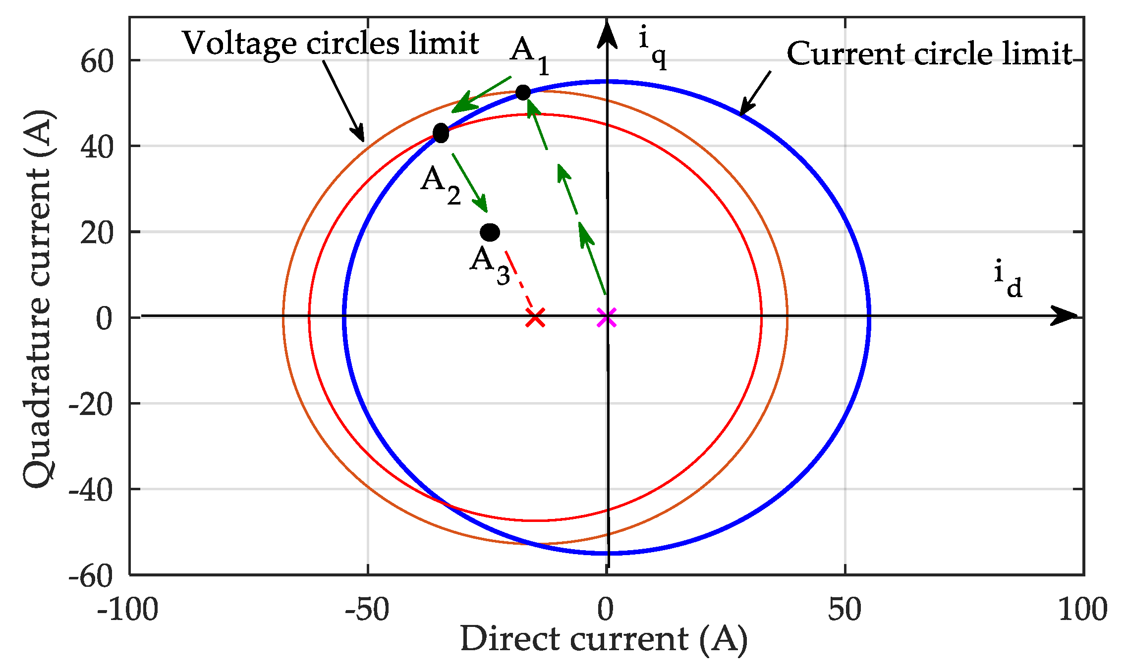
3.1.2. Flux Weakening Control

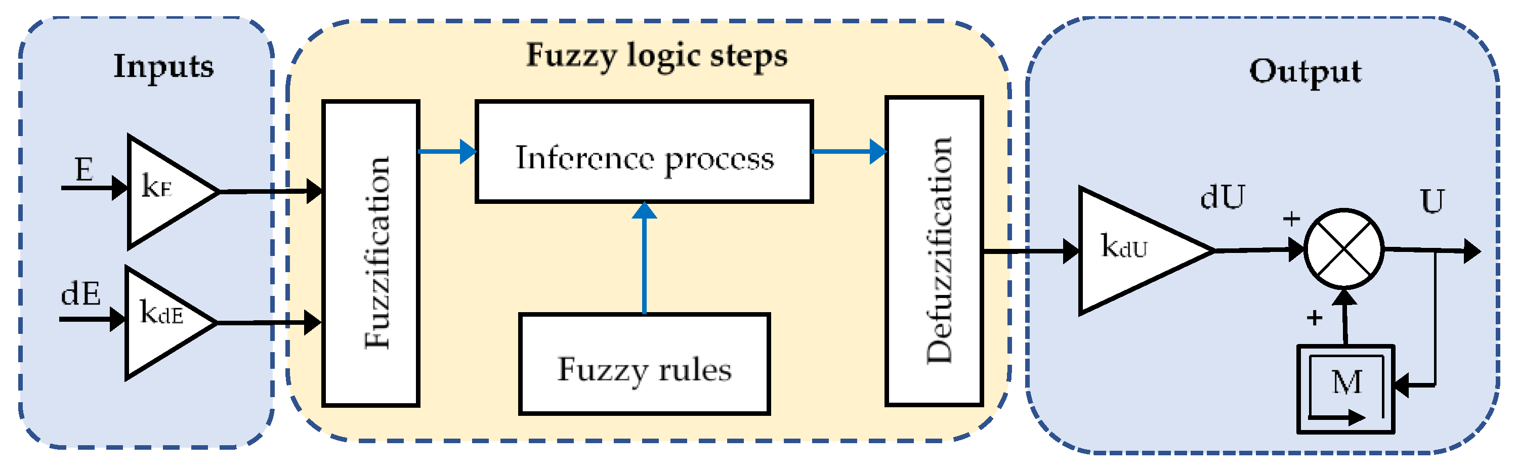
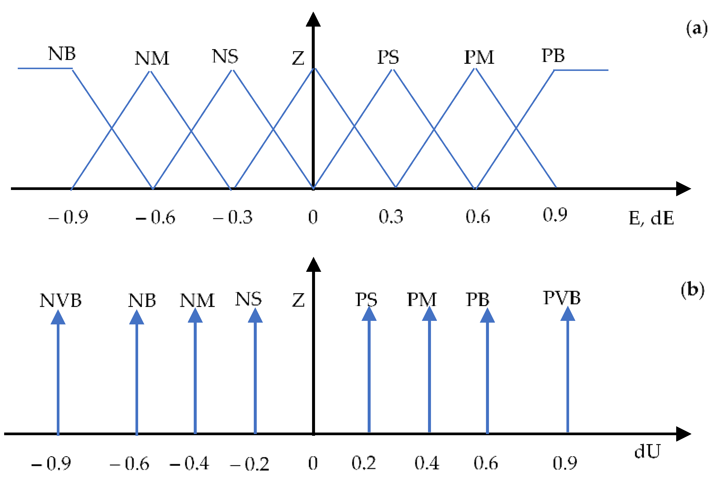
3.1.3. Fuzzy Logic Controller (FLC)


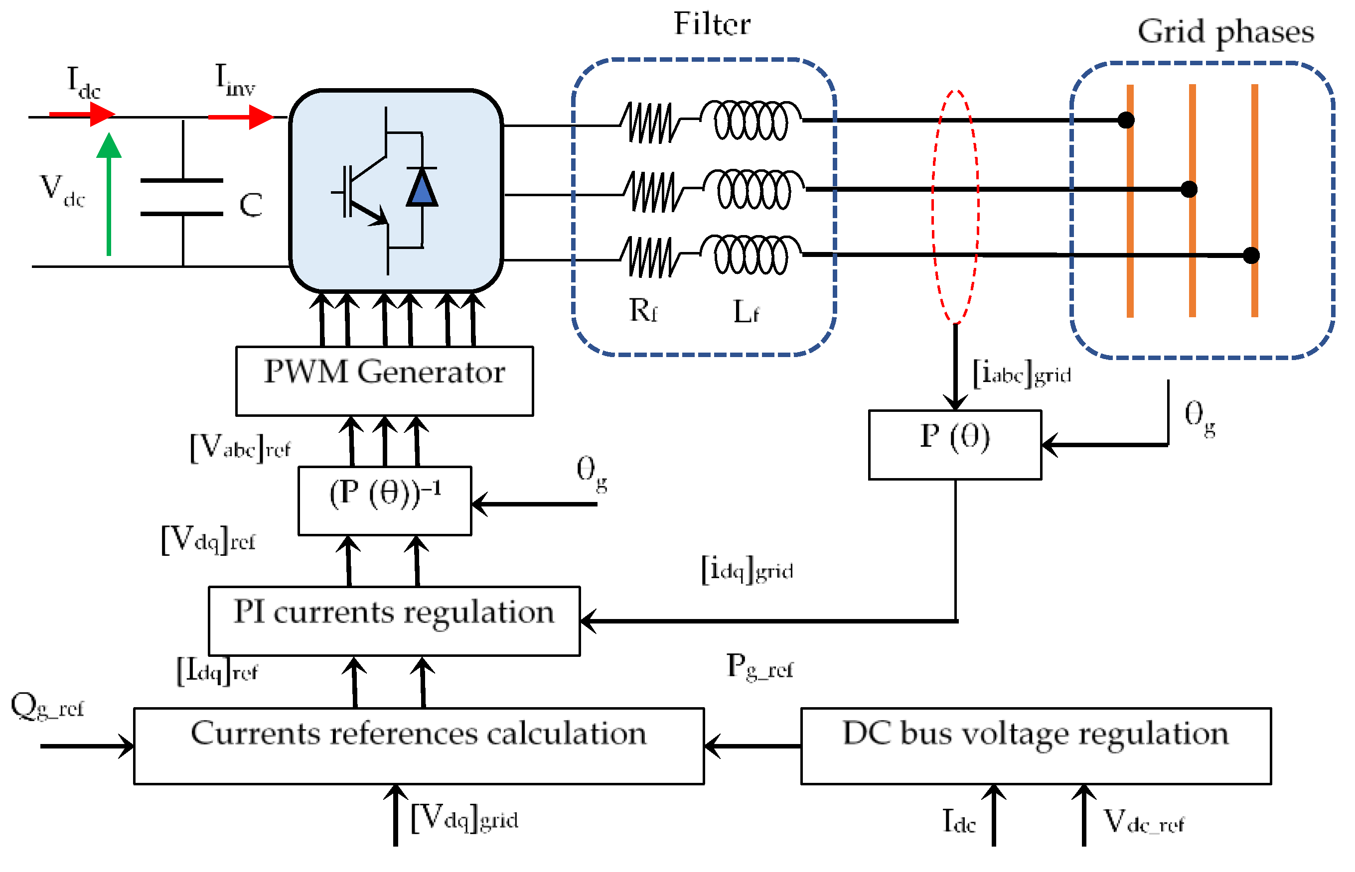
3.2. Grid–Side Inverter Control

4. Simulation Results and Discussion
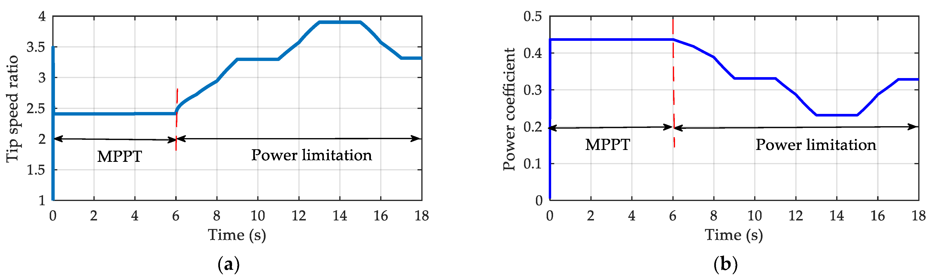
4.1. Wind Turbine


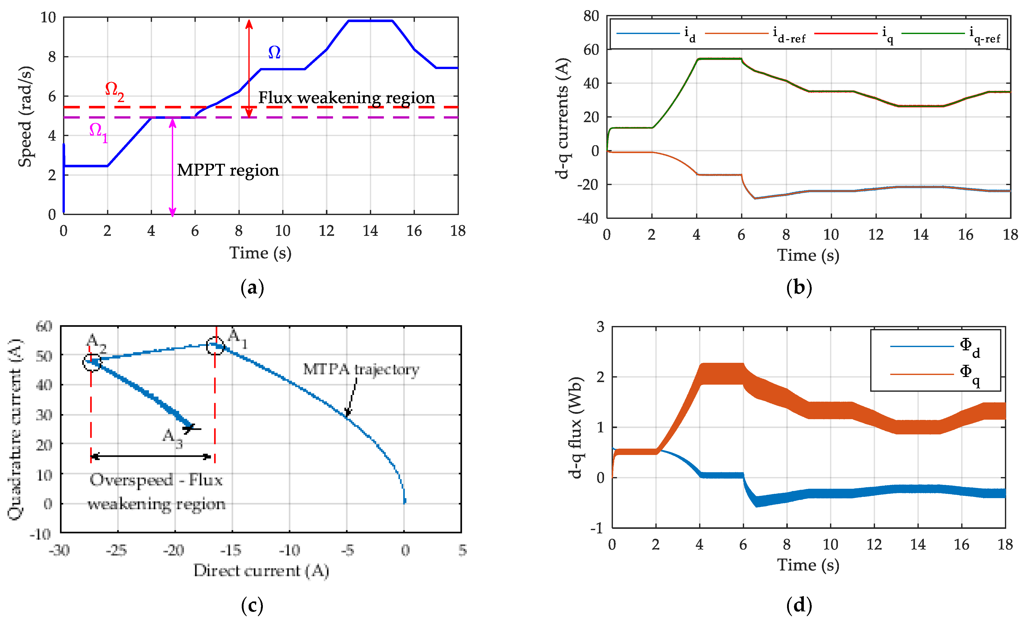
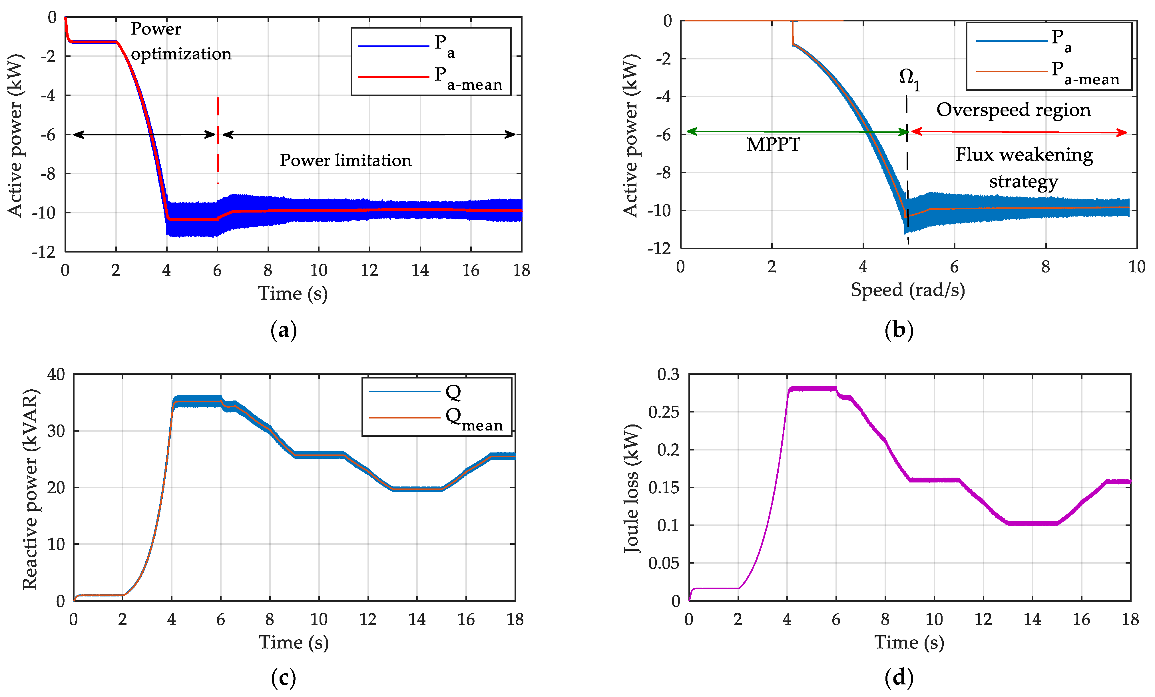
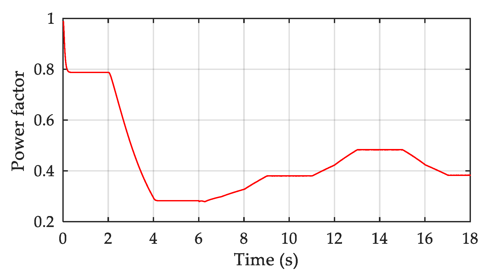
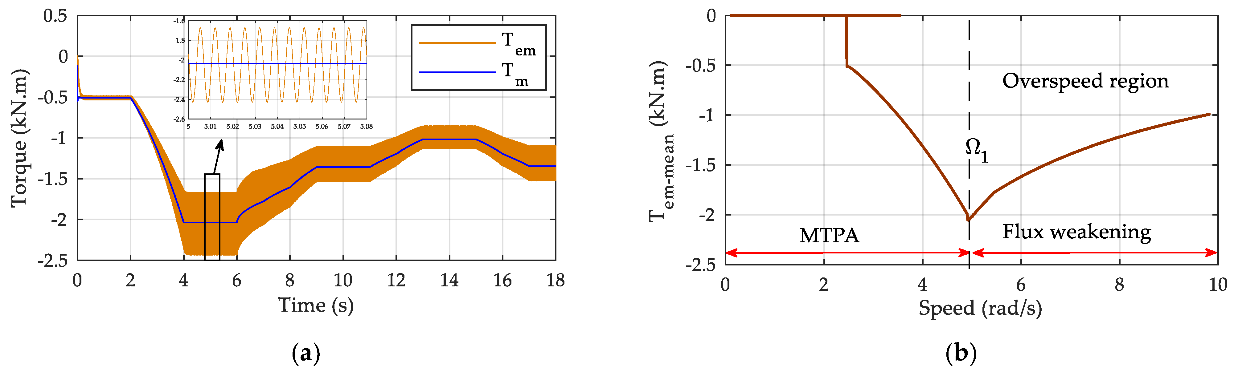
4.2. OR−DSPMG


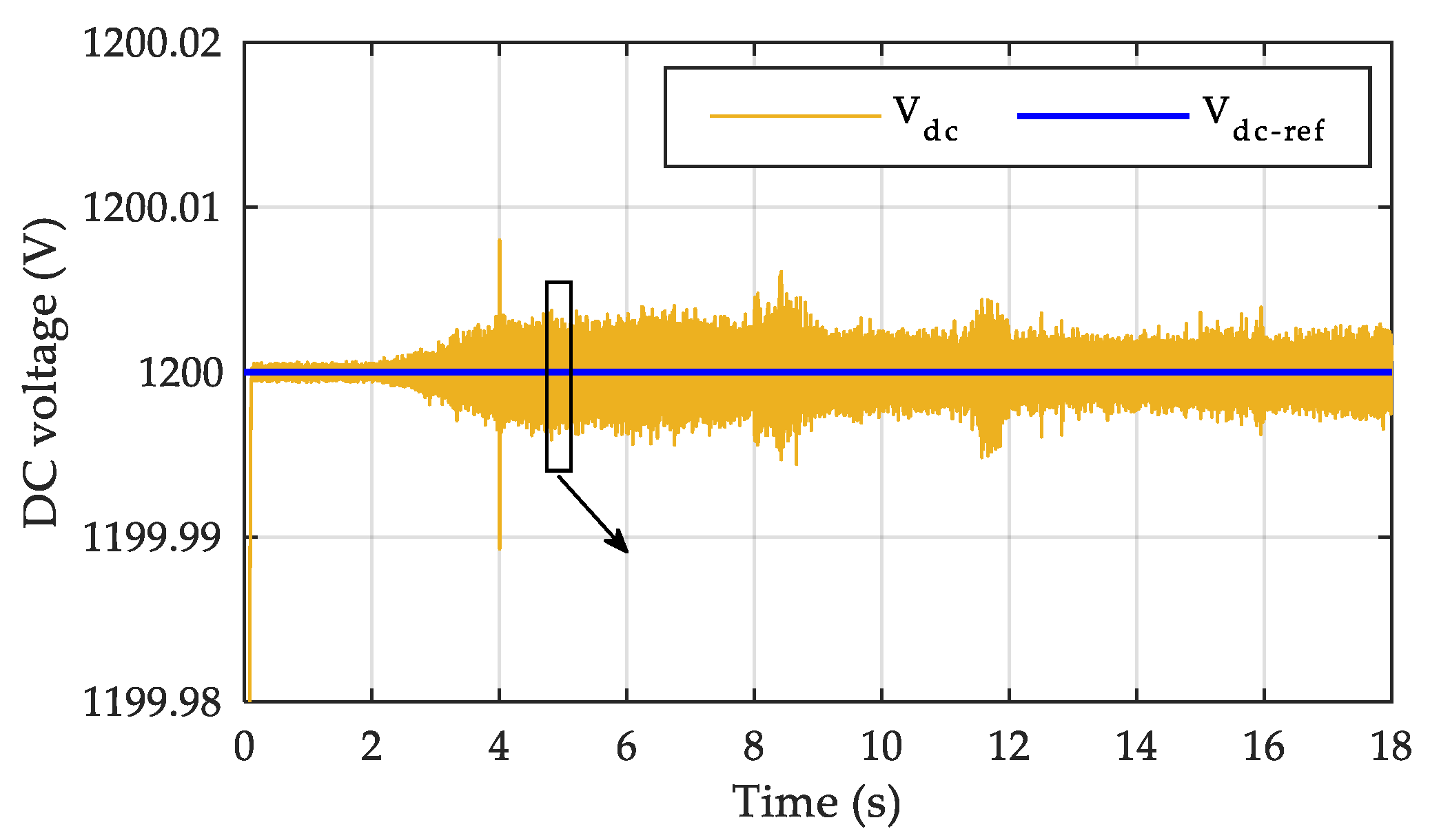
4.3. DC Bus and Grid


5. Conclusions
Author Contributions
Funding
Data Availability Statement
Conflicts of Interest
Appendix A

| Variables | Parameters | |
|---|---|---|
| Wind turbine | vt: wind speed (m/s) | ρ: air density (1.225 kg/m3) |
| Cp: power coefficient | R: wind turbine radius (4.2633 m) | |
| λ: tip speed ratio | Cpmax: maximum power coefficient (0.4369) | |
| Tm: mechanical torque (Nm) | λopt: optimal tip speed ratio (2.41) | |
| Pt: aerodynamic power (kW) | vn: rated wind speed (8.70 m/s) | |
| Pt-max: maximum extracted power (kW) | Pn: rated wind turbine power (10 kW) | |
| Ω: mechanical speed (rpm) | vcut-in: cut-in speed (2.5 m/s) | |
| ΩMPPT: optimal mechanical speed (rad/s) | Number of blade: 3 | |
| OR–DSPMSG | P(θe): Park transformation matrix | Rs: stator resistance (88.37 mΩ) |
| vd, vq: direct and quadrature voltages (V) | L0: continuous self-inductance (25.5 mH) | |
| id, iq: direct and quadrature currents (A) | L1: first harmonic self-inductance (2.5 mH) | |
| φd, φq: direct and quadrature flux (A) | M0: continuous mutual inductance (−12.4 mH) | |
| emd: direct magneto-mortice forces (V) | M1: first harmonic mutual inductance (2.5 mH) | |
| emd: quadrature magneto–mortice forces (V) | φ1: first harmonic PM flux (0.4805 Wb) | |
| we: electrical velocity (rad/s) | Nr: number of teeth in the rotor (64) | |
| θe: electrical position (rad) | Jt: rotor inertia (Nm s−1) | |
| Ld, Lq: direct and quadrature inductance (H) | fv: viscous friction coefficient | |
| Mdq: mutual inductance (H) | Br: PMs magnetization (1.29 T) | |
| Tem: electromagnetic torque (Nm) | µr: relative permeability (1.049) | |
| Tem-mean: average torque value | Em: magnet thickness (27.05 mm) | |
| Tem-max: maximum torque | Ns: stator teeth (48) | |
| Tem-min: minimum torque | Nr: rotor teeth (64) | |
| Cr: torque ripples | Nps: stator pole (12) | |
| Pem: electromagnetic power (kW) | hs: stator teeth depth (7.70 mm) | |
| Pa: active power (kW) | hr: rotor teeth depth (7.70 mm) | |
| Q: reactive power | Es: stator yoke thickness (40.90 mm) | |
| Pcu, Joule loss (kW) | Er: rotor yoke thickness (29.65 mm) | |
| Pir: iron losses (kW) | Rr-out: outer rotor radius (300 mm) | |
| Pa-mean: mean active power (kW) | Ra: slot radius (218.5 mm) | |
| Qmean: mean reactive power (kVAR) | L: axial length (200 mm) | |
| cosψ: power factor | g: air gap thickness (0.5 mm) | |
| Ia(θe): current amplitude (A) | M: active masse (184.4 kg) | |
| Tout: average output torque (3504 Nm) | ||
| n: rated speed (50 rpm) | ||
| DC bus and electrical grid | Vdc: DC bus voltage (V) | Vdc-ref: DC bus voltage reference (1200 V) |
| Idc: converter–side current (A) | C: DC capacitance (8 × 10⁻⁴ F) | |
| Iinv: inverter side current (A) | Rf: filter resistance (0.001 Ω) | |
| Pdc: DC bus active power (kW) | Lf: filter inductance (Lf) | |
| igd, vgd: grid direct current and voltage (A, V) | Vg-rms: voltage RMS value (690 V) | |
| igq, vgq: grid quadrature current and voltage (A, V) | kp: proportional regulator gain (10) | |
| θg: electrical grid angle (rad) | τd: time constant (1 × 10⁻³ s) | |
| Pg,: grid active power (kW) | ||
| Qg: grid reactive power (kVAR) |
| Definition | Numerical Value | |
|---|---|---|
| MTPA and flux weakening | Load angle (θ0) | π/72 |
| Voltage limit (Vlim) | 526 V | |
| Maximum current (Imax) | 45 A | |
| Speed limit Ω1 | 4.9218 rad/s | |
| Speed limit Ω2 | 5.4375 rad/s | |
| Constant: | 0.006 | |
| Constant: | 0.1784 | |
| Fuzzy logic controller | Coefficient: ke | 0.1 |
| Coefficient: kde | 10 | |
| Coefficient: kdu | 100 |
References
- Gökçek, M.; Genç, M. Evaluation of electricity generation and energy cost of wind energy conversion systems (WECSs) in Central Turkey. Appl. Energy 2009, 86, 2731–2739. [Google Scholar] [CrossRef]
- Chen, H.; Zuo, Y.; Chau, K.T.; Zhao, W.; Lee, C.H.T. Modern electric machines and drives for wind power generation: A review of opportunities and challenges. IET Renew. Power Gener. 2021, 15, 1864–1887. [Google Scholar] [CrossRef]
- Chau, K.-T.; Li, W.; Lee, C.H.T. Challenges and Opportunities of Electric Machines for Renewable Energy. Prog. Electromagn. Res. B 2012, 42, 45–74. [Google Scholar] [CrossRef]
- Bang, D.-J.; Polinder, H.; Shrestha, G.; Ferreira, J.A. Promising direct–drive generator system for large wind turbines. In Proceedings of the 2008 Wind Power to the Grid–EPE Wind Energy Chapter 1st Seminar, Delft, The Netherlands, 27–28 March 2008; pp. 1–10. [Google Scholar]
- Boutoubat, M.; Mokrani, L.; Machmoum, M. Control of a wind energy conversion system equipped by a DFIG for active power generation and power quality improvement. Renew. Energy 2013, 50, 378–386. [Google Scholar] [CrossRef]
- Senjyu, T.; Sakamoto, R.; Urasaki, N.; Funabashi, T.; Fujita, H.; Sekine, H. Output power leveling of wind turbine generator for all operating regions by pitch angle control. IEEE Trans. Energy Convers. 2006, 21, 467–475. [Google Scholar] [CrossRef]
- Shafiei, A.; Dehkordi, B.M.; Kiyoumarsi, A.; Farhangi, S. A control approach for a small–scale PMSG–based WECS in the whole wind speed range. IEEE Trans. Power Electron. 2017, 32, 9117–9130. [Google Scholar] [CrossRef]
- Tummala, A.; Velamati, R.K.; Sinha, D.K.; Indraja, V.; Krishna, V.H. A review on small scale wind turbines. Renew. Sustain. Energy Rev. 2016, 56, 1351–1371. [Google Scholar] [CrossRef]
- Morimoto, S.; Takeda, Y.; Hirasa, T.; Taniguchi, K. Expansion of operating limits for permanent magnet motor by current vector control considering inverter capacity. IEEE Trans. Ind. Appl. 1990, 26, 866–871. [Google Scholar] [CrossRef]
- Dehkordi, B.M.; Kiyoumarsi, A.; Hamedani, P.; Lucas, C. A comparative study of various intelligent based controllers for speed control of IPMSM drives in the field-weakening region. Expert Syst. Appl. 2011, 38, 12643–12653. [Google Scholar] [CrossRef]
- Yin, S.; Wang, W. Study on the flux-weakening capability of permanent magnet synchronous motor for electric vehicle. Mechatronics 2016, 38, 115–120. [Google Scholar] [CrossRef]
- Fadel, M.; Sepulchre, L.; Pietrzak-David, M. Deep flux-weakening strategy with MTPV for high-speed IPMSM for vehicle application. IFAC-PapersOnLine 2018, 51, 616–621. [Google Scholar] [CrossRef]
- Akhil, R.S.; Mini, V.P.; Mayadevi, N.; Harikumar, R. Modified flux-weakening control for electric vehicle with PMSM drive. IFAC-PapersOnLine 2020, 53, 325–331. [Google Scholar]
- Zhou, Z.; Scuiller, F.; Charpentier, J.-F.; Benbouzid, M.; Tang, T. Power Control of a nonpitchable PMSG-based marine current turbine at overrated current speed with flux-weakening strategy. IEEE J. Ocean. Eng. 2014, 40, 536–545. [Google Scholar] [CrossRef]
- Djebarri, S.; Charpentier, J.-F.; Scuiller, F.; Benbouzid, M. A Systemic design methodology of PM generators for fixed-pitch marine current turbines. In Proceedings of the 2014 First International Conference on Green Energy (ICGE), Sfax, Tunisia, 25–27 March 2014; pp. 32–37. [Google Scholar]
- Liu, C.; Chau, K.; Jiang, J.; Jian, L. Design of a new outer-rotor permanent magnet hybrid machine for wind power generation. IEEE Trans. Mag. 2008, 44, 1494–1497. [Google Scholar]
- Guerroudj, C.; Saou, R.; Boulayoune, A.; El-hadi Zaïm, M.; Moreau, L. Performance analysis of vernier slotted doubly salient permanent magnet generator for wind power. Int. J. Hydrog. Energy 2017, 42, 8744–8755. [Google Scholar] [CrossRef]
- Bekhouche, L.; Saou, R.; Guerroudj, C.; Kouzou, A.; Zaïm, M.E.H. Electromagnetic torque ripple minimization of slotted doubly-salient-permanent-magnet generator for wind turbine applications. Prog. Electromagn. Res. M 2019, 83, 181–190. [Google Scholar] [CrossRef]
- Saou, R.; Zaïm, M.E.H.; Alitouche, K. Optimal designs and comparison of the doubly salient permanent magnet machine and flux-reversal machine in low-speed applications. Electr. Power Compon. Syst. 2008, 36, 914–931. [Google Scholar] [CrossRef]
- Guerroudj, C.; Boulayoune, A.; Saou, R.; Zaïm, M.E.H.; Moreau, L. Study of vernier effect on the EMF of a slotted DSPM generator for wind power applications. In Proceedings of the International Conference of Renewable Energy (CIER), Sousse, Tunisia, 21–23 December 2015. [Google Scholar]
- Guerroudj, C.; Zaïm, M.E.-H.; Bekhouche, L.; Saou, R.; Rameli, A. Comparison of outer and inner-rotor toothed doubly salient permanent magnet. In Proceedings of the 2019 19th International Symposium on Electromagnetic Fields in Mechatronics, Electrical and Electronic Engineering (ISEF), Nancy, France, 29–31 August 2019; pp. 1–2. [Google Scholar]
- Guerroudj, C.; Karnavas, Y.L.; Charpentier, J.-F.; Chasiotis, I.D.; Bekhouche, L.; Saou, R.; Zaïm, M.E.-H. Design optimization of outer rotor Toothed doubly salient permanent magnet generator using symbiotic organisms search algorithm. Energies 2021, 14, 2055. [Google Scholar] [CrossRef]
- Malekpour, M.; Azizipanah-Abaghooee, R.; Terzija, V. Maximum torque per ampere control with voltage control for IPMSM drive systems. Electr. Power Energy Syst. 2020, 116, 105509. [Google Scholar] [CrossRef]
- Najjar-Khodabakhsh, A.; Soltani, J. MTPA control of mechanical sensorless IPMSM based on adaptive nonlinear control. ISA Trans. 2016, 61, 348–356. [Google Scholar] [CrossRef]
- Aissaoui, A.G.; Tahour, A.; Essounbouli, N.; Nollet, F.; Abid, M.; Chergui, M.I. A fuzzy-PI control to extract an optimal power from wind turbine. Energy Convers. Manag. 2013, 65, 688–696. [Google Scholar] [CrossRef]
- Lokriti, A.; Salhi, I.; Doubabi, S.; Zidani, Y. Induction motor speed drive improvement using fuzzy IP-self-tuning controller. A real time implementation. ISA Trans. 2013, 52, 406–417. [Google Scholar] [CrossRef] [PubMed]
- Njiri, J.G.; Söffker, D. State-of-the-art in wind turbine control: Trends and challenges. Renew. Sustain. Energy Rev. 2016, 60, 377–393. [Google Scholar] [CrossRef]
- Abdullah, M.A.; Yatim, A.H.M.; Tan, C.W.; Saidur, R. A review of maximum power point tracking algorithms for wind energy systems. Renew. Sustain. Energy Rev. 2012, 16, 3220–3227. [Google Scholar] [CrossRef]
- Chen, H.; Tang, T.; Han, J.; Aït-Ahmed, N.; Machmoum, M.; Zaïm, M.E.-H. Current waveforms analysis of toothed pole doubly salient permanent magnet (DSPM) machine for marine tidal current applications. Electr. Power Energy Syst. 2019, 106, 242–253. [Google Scholar] [CrossRef]
- Chen, H.; At-Ahmed, N.; Machmoum, M.; Zam, M.E.H. Modeling and vector control of marine current energy conversion system based on doubly salient permanent magnet generator. IEEE Trans. Sustain. Energy 2015, 7, 409–418. [Google Scholar] [CrossRef]
- Hamrouni, N.; Jraidi, M.; Chérif, A. New control strategy for 2-stage grid–connected photovoltaic power system. Renew. Energy 2008, 33, 2212–2221. [Google Scholar] [CrossRef]
| Output Signal (dU) | Error (E) | |||||||
|---|---|---|---|---|---|---|---|---|
| NB | NM | NS | Z | PS | PM | PB | ||
| Change of error (dE) | NB | NVB | NVB | NVB | NB | NM | NS | Z |
| NM | NVB | NVB | NB | NM | NS | Z | PS | |
| NS | NVB | NB | NM | NS | Z | PS | PM | |
| Z | NB | NM | NS | Z | PS | PM | PB | |
| PS | NM | NS | Z | PS | PM | PB | PVB | |
| PM | NS | Z | PS | PM | PB | PVB | PVB | |
| PB | Z | PS | PM | PB | PVB | PVB | PVB | |
| Time (s) | Ω (rad/s) | id (A) | iq (A) | Φd (Wb) | Φq (Wb) |
|---|---|---|---|---|---|
| 1 | 2.453 | −0.95 | 13.52 | 0.512 | 0.553 |
| 5 | 4.92 | −14.3 | 54.5 | 0.05 | 2.06 |
| Speed (rad/s) | 0.5 × Ω1 | Ω1 | 1.5 × Ω1 | 2.5 × Ω1 |
|---|---|---|---|---|
| Current amplitude (A) | 11.1 | 46 | 33.25 | 26.2 |
| Mean torque value (N.m) | −510 | −2025 | −1298 | −978 |
| Torque ripples (%) | 8.37% | 37.5% | 29.35% | 23.95% |
| Mean active power value (kW) | − 1.265 | −10.230 | −9.705 | −9.680 |
| Joule losses (kW) | 0.016 | 0.281 | 0.146 | 0.091 |
| Mean Reactive power (kVAR) | 0.989 | 34.73 | 23.61 | 17.55 |
| Power factor | 0.79 | 0.28 | 0.38 | 0.48 |
| Base Frequency | Harmonic Order | Voltage (V) | Current (A) |
|---|---|---|---|
| 25 Hz | Fundamental (25 Hz) | 96.48 (100%) | 11.09 (100%) |
| 2nd harmonic (50 Hz) | 13.17 (13.65%) | 0.024 (0.22%) | |
| 4th harmonic (100 Hz) | 0.45 (0.47%) | 0.006 (0.06%) | |
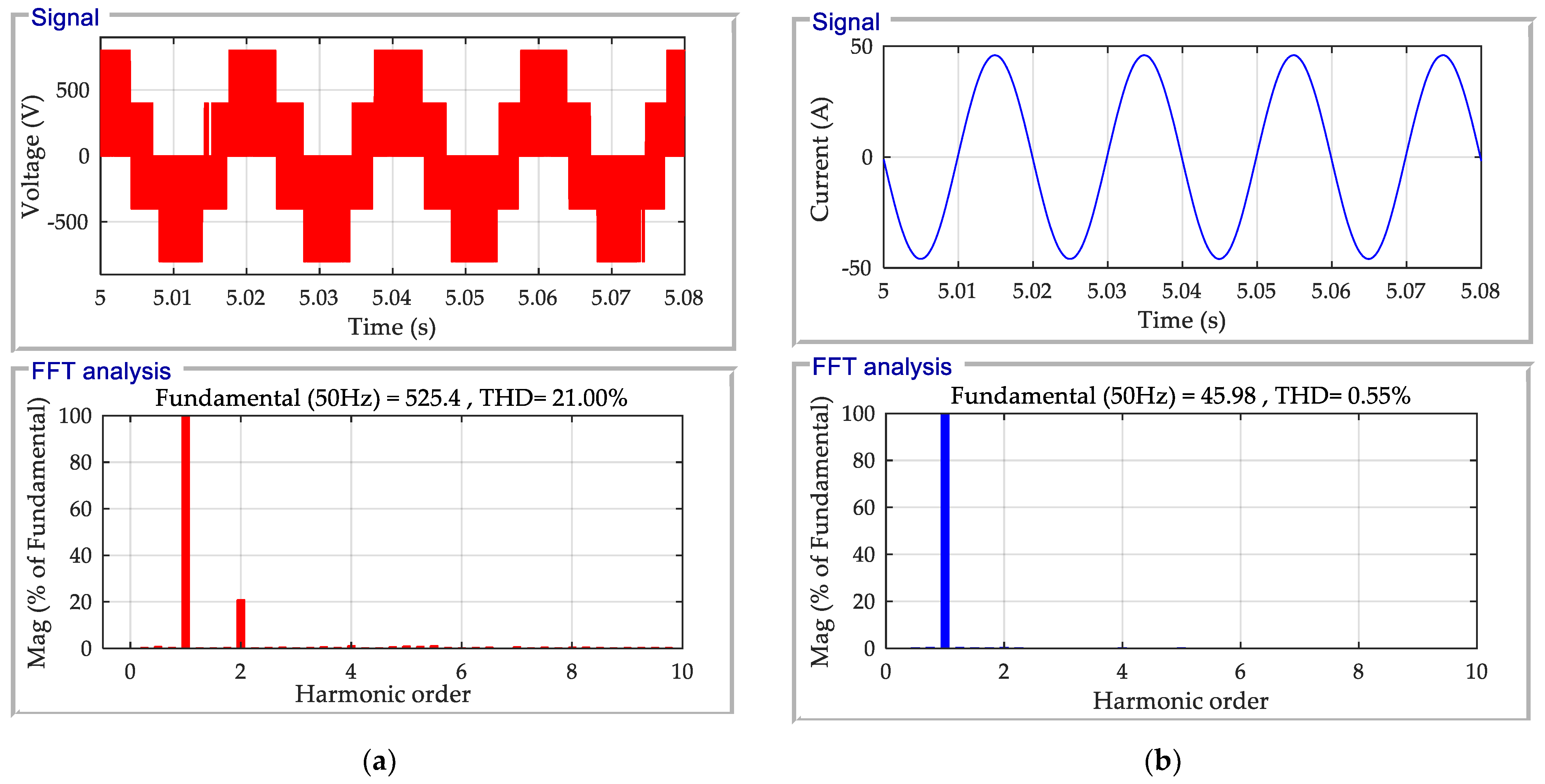
| 50 Hz | Fundamental (50 Hz) | 525.4 (100%) | 45.98 (100%) |
| 2nd harmonic (100 Hz) | 109.33 (20.81%) | 0.15 (0.33%) | |
| 4th harmonic (200 Hz) | 6.83 (1.3%) | 0.06 (0.14%) | |
| 75 Hz | Fundamental (75 Hz) | 516.4 (100%) | 33.22 (100%) |
| 2nd harmonic (150 Hz) | 124.92 (24.19%) | 0.14 (0.44%) | |
| 4th harmonic (300 Hz) | 4.28 (0.83%) | 0.03 (0.10%) | |
| 100 Hz | Fundamental (100 Hz) | 506.9 (100%) | 26.16 (100%) |
| 2nd harmonic (200 Hz) | 137.57 (27.14%) | 0.15 (0.60%) | |
| 4th harmonic (400 Hz) | 12.92 (2.55%) | 0.04 (0.16%) |
Disclaimer/Publisher’s Note: The statements, opinions and data contained in all publications are solely those of the individual author(s) and contributor(s) and not of MDPI and/or the editor(s). MDPI and/or the editor(s) disclaim responsibility for any injury to people or property resulting from any ideas, methods, instructions or products referred to in the content. |
© 2023 by the authors. Licensee MDPI, Basel, Switzerland. This article is an open access article distributed under the terms and conditions of the Creative Commons Attribution (CC BY) license (https://creativecommons.org/licenses/by/4.0/).
Share and Cite
Remli, A.; Guerroudj, C.; Charpentier, J.-F.; Kendjouh, T.; Bracikowski, N.; L. Karnavas, Y. Control of an Outer Rotor Doubly Salient Permanent Magnet Generator for Fixed Pitch kW Range Wind Turbine Using Overspeed Flux Weakening Operations. Actuators 2023, 12, 168. https://doi.org/10.3390/act12040168
Remli A, Guerroudj C, Charpentier J-F, Kendjouh T, Bracikowski N, L. Karnavas Y. Control of an Outer Rotor Doubly Salient Permanent Magnet Generator for Fixed Pitch kW Range Wind Turbine Using Overspeed Flux Weakening Operations. Actuators. 2023; 12(4):168. https://doi.org/10.3390/act12040168
Chicago/Turabian StyleRemli, Aziz, Cherif Guerroudj, Jean-Frédéric Charpentier, Tarek Kendjouh, Nicolas Bracikowski, and Yannis L. Karnavas. 2023. "Control of an Outer Rotor Doubly Salient Permanent Magnet Generator for Fixed Pitch kW Range Wind Turbine Using Overspeed Flux Weakening Operations" Actuators 12, no. 4: 168. https://doi.org/10.3390/act12040168
APA StyleRemli, A., Guerroudj, C., Charpentier, J.-F., Kendjouh, T., Bracikowski, N., & L. Karnavas, Y. (2023). Control of an Outer Rotor Doubly Salient Permanent Magnet Generator for Fixed Pitch kW Range Wind Turbine Using Overspeed Flux Weakening Operations. Actuators, 12(4), 168. https://doi.org/10.3390/act12040168