A Decentralized LQR Output Feedback Control for Aero-Engines

Abstract

Aero-engine control systems generally adopt centralized or distributed control schemes, in which all or most of the tasks of the control system are mapped to a specific processor for processing. The performance and reliability of this processor have a significant impact on the control system. Based on the aero-engine distributed control system (DCS), we propose a decentralized controller scheme. The characteristic of this scheme is that a network composed of a group of nodes acts as the controller of the system, so that there is no core control processor in the system, and the computation is distributed throughout the entire network. An LQR output feedback control is constructed using system input and output, and the control tasks executed on each node in the decentralized controller are obtained. The constructed LQR output feedback is equivalent to the optimal LQR state feedback. The primal-dual principle is used to tune the parameters of each decentralized controller. The parameter tuning algorithm is simple to calculate, making it conducive for engineering applications. Finally, the proposed scheme was verified by simulation. The simulation results show that a high-precision feedback gain matrix can be obtained with a maximum of eight iterations. The parameter tuning algorithm proposed in this paper converges quickly during the calculation process, and the constructed output feedback scheme achieves equivalent performance to the state feedback scheme, demonstrating the effectiveness of the design scheme proposed in this paper.

1. Introduction

Early aero-engine control systems adopt a centralized control scheme, where the controller is connected to analog sensors and actuators via cables [1]. The controller executes tasks such as calculation of control law, analog-to-digital conversion (ADC), and digital-to-analog conversion (DAC), resulting in a large workload for the controller. Meanwhile, the centralized control scheme increases the difficulty and cost of upgrading and maintaining the aero-engine throughout its entire lifespan [2]. Moreover, the cables should be arranged around the rotating components. The huge quantity of cables reduces the thrust-to-weight ratio of the aero-engine. To overcome the drawbacks of the centralized control scheme, distributed control schemes for aero-engines have emerged [3].

A distributed control system (DCS) is a control architecture applied in process control or plant control [4,5,6,7]. In an aero-engine DCS, traditional analog sensors and actuators have been replaced by intelligent digital sensors and actuators. The components in the control system are connected through a universal and standardized communication interface [8,9]. Currently, aero-engine related enterprises and scientific research institutions have a basic consensus on the “functional decentralization” of the DCS, that is, some of the functions of the controller in the centralized control system, such as signal conditioning and status monitoring, are executed by intelligent sensors and actuators, while the central controller focuses on executing the core control functions of the system [10]. A simple and robust digital bus replaces the large number of cables connecting the aero-engine control components to the avionics [11,12]. Compared with centralized control, an aero-engine DCS possesses the following advantages [13]: (1) Digital intelligent sensors and actuators reduce the workload of the central controller; (2) The digital bus reduces the weight of the aero-engine control system; (3) The modular design scheme reduces the difficulty and cost of system maintenance and upgrades.

Although the aero-engine DCS has the above advantages, it still has some inherent disadvantages due to the existence of core nodes.

• With the improvement of aero-engine performance, the function and complexity of control tasks have greatly increased, which has increased the workload of controller. The control system needs to use high-performance, multi-core processors as its controller, which in turn puts relatively high demands on the thermal management system of the aero-engine.
• The amount of software code in aero-engine control systems is increasing rapidly, which significantly impacts the software reliability.
• The core control tasks of the aero-engine, such as control-law calculation, are executed in the central controller. The central controller determines the performance of the entire aero-engine control system, and its failure or damage has significant impact on the aero-engine or even the aircraft.

Decentralizing the central controller is an effective way to overcome the shortcomings of the aero-engine DCS.

Output feedback and state feedback are both utilized in designing closed-loop control systems. Generally, output feedback is easier to implement in projects, but state feedback offers better performance. However, state feedback requires full system states. In the case of aero-engines, there are numerous state variables, some of which are hard to measure. Furthermore, some state variables may possess only mathematical meaning without a physical value. Therefore, the application of the aero-engine state feedback is restricted.

Linear quadratic regulation (LQR) can derive the optimal control law for linear state feedback and facilitate the implementation of optimal closed-loop control [14]. Optimum LQR control design is achieved by solving the LQR problem [15,16,17]. The conventional approach to the LQR problem involves solving the Bellman equation through dynamic programming. For linear control system design, it is transformed into the solution of the algebraic Riccati equation (ARE). Both the Bellman equation and ARE are challenging to solve [18,19], and it is difficult to use a conventional microprocessor for real-time calculation [20,21,22,23,24].

The contributions of this paper are as follows. Based on the aero-engine DCS, we propose a decentralized controller architecture. An LQR output feedback control was constructed through system input and output, and the control tasks executed on each node in the decentralized controller are obtained. The constructed LQR output feedback is equivalent to the optimal LQR state feedback. Finally, a simple linear iterative algorithm for solving the LQR problem is introduced. It is demonstrated that the calculation of the decentralized control tasks is simple and the LQR output feedback provides equivalent performance to the LQR optimal state feedback. Meanwhile, the LQR solving algorithm is simple to calculate and fast to converge.

The remainder of this paper is organized as follows. Section 2 introduces an aero-engine linear state space model. Section 3 introduces the output feedback scheme of the decentralized control system. Section 4 introduces an output feedback scheme based on the Q-Learning LQR, equivalent to the state feedback scheme. Section 5 introduces a primal-dual principle-based parameter-tuning algorithm. Section 6 presents the simulation of the scheme proposed in this paper. Finally, Section 7 is the last section of this paper, providing the summary and conclusion.

2. Aero-Engine Model

Turbofan engines are widely used in both military and civil aviation [25,26] due to their high efficiency. However, the technical difficulty is also high [27,28], and they require advanced control systems. Here, we consider the turbofan engine as an example to study [29]. Figure 1 is the schematic diagram of a turbofan engine. We first introduced the nonlinear modeling of the turbofan engine. Then, we derived a linearized model based on the nonlinear model and obtained the structure of the linearized model. Finally, we introduced the identification of the model parameters based on the input and output data of the engine.

2.1. Nonlinear Modeling

Due to the strong nonlinear characteristics of aero-engines, the nonlinear model of the aero-engines is briefly analyzed in this section. Based on fundamental physical principles, we model the various components of the turbofan engine. Then, using aerothermodynamic principles among components and the common working conditions of associated components, we establish joint equations. The following is a brief introduction to the physical equations involved.

(1)

Intake

The intake is the first part where the air flows through the aero-engine.

The inlet temperature $T_2$ and the pressure $P_2$ of the aero-engine are:

$$\left\{\begin{array}{l}{T}_2=T_1\left(1+\frac{k_1-1}{2}·{Ma}^2\right)\\ P_2={\sigma }_1{P}_1{\left(1+\frac{k_1-1}{2}·{Ma}^2\right)}^{k_1/k_1-1}\end{array}\right.$$

(1)

where $T_1$ and $P_1$ are the total air temperature and the total pressure at the intake, respectively, $k_1$ is the air adiabatic index, ${\sigma }_1$ is the total pressure recovery coefficient of the intake, $M_a$ is Mach number.

(2)

Fan

The fan outlet temperature $T_{21}$ and the pressure $P_{21}$ of the aero-engine are:

$$\left\{\begin{array}{l}{T}_{21}=T_2\left(1+\frac{{\pi }_F^{\frac{k_F-1}{k_F}}-1}{{\eta }_F}\right)\\ P_{21}={\pi }_F{P}_2\end{array}\right.$$

(2)

where $k_F$ is the air adiabatic index, ${\pi }_F$ is the fan pressure ratio, ${\eta }_F$ is the efficiency of the fan.

(3)

Compressor

The compressor outlet temperature $T_3$ and the pressure $P_3$ are:

$$\left\{\begin{array}{l}{T}_3=T_{22}\left(1+\frac{{\pi }_C^{\frac{k_C-1}{k_C}}-1}{{\eta }_C}\right)\\ P_3={\pi }_C{P}_{22}\end{array}\right.$$

(3)

where $T_{22}$ and $P_{22}$ are the temperature and pressure of the compressor inlet, respectively, $k_C$ is the air adiabatic index, ${\pi }_C$ is the compressor pressure ratio, ${\eta }_C$ is the efficiency of the compressor.

(4)

Combustion chamber

The outlet pressure of the combustion chamber $P_4$ can be expressed by the following equation:

$$P_4={\sigma }_3{P}_4$$

(4)

where ${\sigma }_3$ represents the total pressure recovery coefficient of the combustion chamber.

(5)

High-pressure turbine

The outlet temperature $T_{41}$ and pressure $P_{41}$ of the high-pressure turbine can be obtained as:

$$\left\{\begin{array}{l}{T}_{41}=\frac{q_{mg,TH}{T}_4+C_{HPTCool}{q}_{maC,totalTcool}}{q_{mg,TH,total}}\left(1-\left(1-{\pi }_{TH}^{\frac{1-k_{TH}}{k_{TH}}}\right){\eta }_{TH}\right)\\ P_{41}=\frac{P_4}{{\pi }_{TH}}\end{array}\right.$$

(5)

where $q_{mg,TH}$ is the gas flow converted by the high-pressure turbine, $T_4$ is the outlet temperature of the combustion chamber, $C_{HPTCool}$ is the proportion coefficient of the high-pressure compressor bleed air used to cool the high-pressure turbine, $q_{maC,totalTcool}$ is the total flow of added air, $q_{mg,TH,total}$ is the outlet air flow of the high-pressure turbine, ${\pi }_{TH}$ is the high-pressure turbine pressure ratio, ${\eta }_{TH}$ is the efficiency of the high-pressure turbine, $k_{TH}$ is the gas adiabatic index.

(6)

Low-pressure turbine

The outlet temperature $T_5$ and pressure $P_5$ of the low-pressure turbine are calculated by the following equations:

$$\left\{\begin{array}{l}{T}_5=\frac{q_{mg,TL}{T}_{42}+C_{LPTCool}{q}_{maC,totalTcool}}{q_{mg,TL,total}}\left(1-\left(1-{\pi }_{TL}^{\frac{1-k_{TL}}{k_{TL}}}\right){\eta }_{TL}\right)\\ P_5=\frac{P_{42}}{{\pi }_{TL}}\end{array}\right.$$

(6)

where $q_{mg,TL}$ is the gas flow converted by the high-pressure turbine, $T_{42}$ is the inlet temperature of the low-pressure turbine, $C_{LPTCool}$ is the proportion coefficient of the high-pressure compressor bleed air used to cool the low-pressure turbine, $q_{mg,TL,total}$ is the outlet air flow of the low-pressure turbine, ${\pi }_{TL}$ is the low-pressure turbine pressure ratio, ${\eta }_{TL}$ is the efficiency of the low-pressure turbine, $k_{TL}$ is the gas adiabatic index.

(7)

Bypass duct

The temperature $T_6$ and the pressure $P_6$ of the outlet of the bypass duct are:

$$\left\{\begin{array}{l}{T}_6=T_{21}\\ P_6={\sigma }_4{P}_{21}\end{array}\right.$$

(7)

where $T_{21}$ and $P_{21}$ are the outlet temperature and pressure of the fan, respectively, ${\sigma }_4$ is the total pressure recovery coefficient of the bypass duct.

(8)

Mixer

The gas flow $q_{mg,7}$ at the outlet of the mixer is the sum of the air flow $q_{ma,6}$ at the outlet of the bypass duct and the gas flow $q_{mg,5}$ at the outlet of the low-pressure turbine. Let ${\sigma }_5$ denotes the total pressure recovery coefficient of the mixer, then the physical parameters at the outlet of the mixer are:

$$\left\{\begin{array}{l}{q}_{mg,7}=q_{mg,5}+q_{ma,6}\\ h_7=\frac{h_5{q}_{mg,5}+h_6{q}_{ma,6}}{q_{mg,7}}\\ P_7={\sigma }_5·\frac{P_5{q}_{mg,5}+P_6{q}_{ma,6}}{q_{mg,7}}\end{array}\right.$$

(8)

where $h_5$, $h_6$, and $h_7$ are the specific enthalpy of the gas at the outlet of the low-pressure turbine, air at the outlet of the bypass duct, and gas at the outlet of the mixer, respectively. From $h_7$, it is easy to obtain the temperature $T_7$ at the outlet of the mixer.

(9)

Nozzle

The gas flow $q_{mg,8}$ at the nozzle outlet is:

$$q_{mg,8}=K_q\frac{P_8{A}_{8}q\left({\lambda }_8\right)}{\sqrt{T_7}}$$

(9)

where $K_q$ is the state coefficient of the nozzle, $q\left({\lambda }_8\right)$ refers to the function related to the characteristics of the bypass duct and the core duct, $A_8$ is the sectional area of the nozzle, $T_7$ is the outlet temperature of the mixer.

The high-pressure turbine drives the high-pressure compressor of the turbofan engine to form the high-pressure rotor. The low-pressure turbine drives the fan to form the low-pressure rotor. After passing through the intake and fan, the gases enter the bypass duct and the core duct, respectively. The common working equations of the turbofan engine are obtained according to the flow, pressure, and power balance between the engine components.

(1)

High-pressure rotor power balance

$$P_H=P_{CH}+P_{ex,H}+D_H\left(\frac{d{n}_H}{dt}\right)$$

(10)

where $P_H$ denotes the high-pressure turbine power, $P_{CH}$ denotes the high-pressure compressor power, $P_{ex,H}$ denotes the power lost by transmission friction force, $D_H\left(\frac{d{n}_H}{dt}\right)$ denotes the high-pressure rotor acceleration power. Furthermore, $D_H={\left(\pi /30\right)}^2{J}_H{n}_H$, $J_H$ denotes the moment of inertia of the high-pressure rotor, $n_H$ denotes the speed of the high-pressure rotor.

When the aero-engine is stable, $d{n}_H/dt=0.$ Ignoring the power lost by transmission friction force $P_{ex,H}$, Equation (10) can be simplified as:

$$P_H=P_{CH}$$

(11)

(2)

Low-pressure rotor power balance

Similar to the high-pressure rotor, when the aero-engine is stable, ignoring the power lost by transmission friction force, we can obtain:

$$P_L=P_{CL}$$

(12)

where $P_L$ denotes the low-pressure turbine power, $P_{CL}$ denotes the low-pressure compressor power.

(3)

Fan air flow balance

After flowing through the fan, the gas is divided into two parts, one part enters the bypass duct and the other enters the high-pressure compressor. Ignoring the gas flow loss, then:

$$q_{maF}=q_{maC}+q_{ma6}$$

(13)

where $q_{maF}$ is the air flow from the fan, $q_{maC}$ is the air flow into the high-pressure compressor, $q_{ma6}$ is the air flow into the bypass duct.

(4)

High-pressure turbine gas flow balance

$$q_{mg,4}=q_{maC}+q_{mf}$$

(14)

where $q_{mg,4}$ is the gas flow into the high-pressure turbine, $q_{maC}$ is the gas flow from the high-pressure compressor, $q_{mf}$ is the fuel flow.

(5)

Low-pressure turbine gas flow balance

The low-pressure turbine inlet gas flow is equal to the high-pressure turbine outlet gas flow $q_{mg,42}$:

$$q_{mg,42}=q_{mg,4}+C_{HPTCool}{q}_{maC,totalTcool}$$

(15)

where $C_{HPTCool}$ is the proportion coefficient of the high-pressure compressor bleed air used to cool the high-pressure turbine, $q_{maC,totalTcool}$ is the total air flow into the high-pressure turbine.

(6)

Nozzle gas flow balance

$$q_{mg,8}=q_{mg,5}+q_{ma,16}$$

(16)

where $q_{mg,8}$ is the gas flow at the inlet of the nozzle, $q_{mg,5}$ is the gas flow at the low-pressure turbine outlet, $q_{ma,16}$ is the gas flow into the bypass duct.

2.2. Linear State Space Model

We derived the component-level nonlinear model of the aero-engine, along with the common working equations. However, the current control system is primarily designed based on a linear system. Therefore, a linear model of the aero-engine is needed. In this section, the system identification method is applied to obtain the model of the aero-engine. Firstly, the structural identification of the model is carried out.

The state equation and the output equation of the aero-engine nonlinear state space model are:

$$\left\{\begin{array}{l}\dot{x}=f\left(x,u\right)\\ y=g\left(x,u\right)\end{array}\right.$$

(17)

where $x$ is the state vector, $y$ is the output vector, $u$ is the control input, and the dimensions of $x$, $y$, $u$ are $n$, $m$, $r$, respectively. It is assumed that the state equation and the output equation of the aero-engine are differentiable within the flight envelope.

Based on the principle of rotor dynamics, taking the aero-engine as a rigid body, let $\dot{w}$ denote the angular acceleration, $\Delta Q$ denote the torque difference between the two shafts, and $I$ denote the mass moment of inertia. The acceleration of the system can be obtained from Newtonian mechanics as:

$$\dot{w}=\frac{\Delta Q}{I}$$

(18)

Let $N$ denote the aero-engine shaft speed, $f$ is the function between shaft speed and fuel quantity, the aero-engine shaft dynamic equation is:

$$\dot{n}=\frac{f\left(N,W_f\right)}{I}$$

(19)

Let $J_H$ denote the moment of inertia of the high-pressure rotor, $\Delta M_H$ the residual torque of the high-pressure rotor, $J_L$ the moment of inertia of the low-pressure rotor, $\Delta M_L$ the residual torque of the low-pressure rotor, then, there are two rotor moment balance equations for the aero-engine:

$$\left\{\begin{array}{l}\left(\frac{\pi }{30}\right)·J_H·\frac{d{N}_C}{dt}=\Delta M_H\\ \left(\frac{\pi }{30}\right)·J_L·\frac{d{N}_F}{dt}=\Delta M_L\end{array}\right.$$

(20)

The residual torque of the high-pressure rotor and the residual torque of the low-pressure rotor are:

$$\left\{\begin{array}{l}\Delta M_H=M_{TH}-M_{CH}=\Delta M_H·\left(N_C,N_F,W_f\right)\\ \Delta M_L=M_{TL}-M_{CL}=\Delta M_L·\left(N_C,N_F,W_f\right)\end{array}\right.$$

(21)

Linearization is carried out at a steady-state operating point $\left(x_0,u_0\right)$ of the aero-engine:

$$\left\{\begin{array}{l}\Delta M_H={\left.\frac{\partial \Delta M_H}{\partial N_C}\right|}_{\left(x_0,u_0\right)}\Delta N_C+{\left.\frac{\partial \Delta M_H}{\partial N_F}\right|}_{\left(x_0,u_0\right)}\Delta N_F+{\left.\frac{\partial \Delta M_H}{\partial W_f}\right|}_{\left(x_0,u_0\right)}\Delta W_f\\ \Delta M_L={\left.\frac{\partial \Delta M_L}{\partial N_C}\right|}_{\left(x_0,u_0\right)}\Delta N_C+{\left.\frac{\partial \Delta M_L}{\partial N_F}\right|}_{\left(x_0,u_0\right)}\Delta N_F+{\left.\frac{\partial \Delta M_L}{\partial W_f}\right|}_{\left(x_0,u_0\right)}\Delta W_f\end{array}\right.$$

(22)

From Equations (20) and (22), the linearized shaft dynamic equation is:

$$\left\{\begin{array}{l}{\dot{N}}_C=a_{11}·\Delta N_C+a_{12}·\Delta N_F+b_{11}·\Delta W_f\\ {\dot{N}}_F=a_{21}·\Delta N_C+a_{22}·\Delta N_F+b_{21}·\Delta W_f\end{array}\right.$$

(23)

where

$$\begin{array}{l}{a}_{11}=\left(\frac{30}{\pi ·J_H}\right)·{\left.\frac{\partial \Delta M_H}{\partial N_C}\right|}_{\left(x_0,u_0\right)}\\ a_{12}=\left(\frac{30}{\pi ·J_H}\right)·{\left.\frac{\partial \Delta M_H}{\partial N_F}\right|}_{\left(x_0,u_0\right)}\\ a_{21}=\left(\frac{30}{\pi ·J_L}\right)·{\left.\frac{\partial \Delta M_L}{\partial N_C}\right|}_{\left(x_0,u_0\right)}\\ a_{22}=\left(\frac{30}{\pi ·J_L}\right)·{\left.\frac{\partial \Delta M_L}{\partial N_F}\right|}_{\left(x_0,u_0\right)}\\ b_{11}=\left(\frac{30}{\pi ·J_H}\right)·{\left.\frac{\partial \Delta M_H}{\partial w_f}\right|}_{\left(x_0,u_0\right)}\\ b_{22}=\left(\frac{30}{\pi ·J_L}\right)·{\left.\frac{\partial \Delta M_L}{\partial W_f}\right|}_{\left(x_0,u_0\right)}\end{array}$$

Equation (23) can be written as:

$$\left\{\begin{array}{l}\dot{x}=Ax+Bu\\ y=Cx+Du\end{array}\right.$$

(24)

where $x$, $y$, $u$ are the state vector, the output vector, and the control input of the aero-engine state space model, respectively. The model described by Equation (24) is a second-order system, and the structural identification of the system model is completed. The linear model of the turbofan engine is represented as a second-order system. Next, we introduce the method for identifying the parameters of the system model.

MATLAB software was used for identification. By running the open-loop control system of the engine model and providing an input at a certain steady-state point, the input and output data of the model can be saved when the system stabilizes, thus obtaining the data from the engine at that steady-state point. Then, a small step signal based on the input data is added to each variable, and the input and output data are saved when the system reaches a steady state. By subtracting the input and output data of the steady-state point from the input and output data of the system’s step response, incremental data can be obtained that can be used for identification. After preprocessing the data, it is imported into the system identification toolbox, and the N4SID method is used to identify the linear model of the system.

Based on the method of system identification described above, we provide two linear models of the turbofan engine.

The first is a single-variable model for the turbofan engine. Here, taking the high-pressure rotor-speed control as an example, the high-pressure rotor speed $y=N_h$ is the controlled variable of the control system, and the main fuel flow $u=W_f$ is the control input. The system identification in this section is based on the input and output data of the system, i.e., the model of the turbofan engine is a black-box model, and the specific meaning of the state variables in the model is not limited. At the steady-state point where the relative speed is 85%, height $H=0$, mach number $M_a=0$, and the sample time is 20 ms, the discrete time linear state space model of the turbofan engine obtained through the system identification is:

$$\left\{\begin{array}{l}x\left[k+1\right]=G_{S}x\left[k\right]+H_{S}u\left[k\right]\\ y\left[k\right]=C_{S}x\left[k\right]+D_{S}u\left[k\right]\end{array}\right.$$

(25)

where $x={\left[\begin{array}{cc}{x}_1& x_2\end{array}\right]}^T$ is the state variable, which has no physical meaning. Because this is not a physical variable, it cannot be directly measured by the sensors. Therefore, the model established by Equation (25) cannot theoretically realize state feedback control by conventional methods.

The coefficient matrix of Equation (25) is:

$$\left\{\begin{array}{l}{G}_S=\left[\begin{array}{cc}{g}_{11}& g_{12}\\ g_{21}& g_{22}\end{array}\right]=\left[\begin{array}{cc}0.9854& 0.0156\\ -1.3474& 0.5935\end{array}\right]\\ H_S=\left[\begin{array}{c}{h}_{11}\\ h_{21}\end{array}\right]=\left[\begin{array}{c}0.1875\\ 19.3024\end{array}\right]\\ C_S=\left[\begin{array}{cc}1& 0\end{array}\right]\\ D_S=0\end{array}\right.$$

The second presented system is a multi-variable model for the turbofan engine. Here, the target of the control system is set to achieve a change in the thrust of the turbofan engine according to the angle of the throttle lever. As thrust cannot be measured through the sensors, parameters that are highly correlated with thrust are selected to represent the thrust characteristics. Here, according to the aero-engine principle, the controlled variable can be selected as high-pressure rotor speed $n_H$ and turbine pressure ratio $P_{i}T={\pi }_{TL}{\pi }_{TH}$, the reference input is selected as fuel flow $W_f$ and nozzle area $A_8$. At the steady-state point with the power lever angle $PLA=35°$, height $H=0$, mach number $M_a=0$, sample time 20 ms, the discrete time linear state space model of the turbofan engine obtained through the system identification is:

$$\left\{\begin{array}{l}x\left[k+1\right]=G_{M}x\left[k\right]+H_{M}u\left[k\right]\\ y\left[k\right]=C_{M}x\left[k\right]+D_{M}u\left[k\right]\end{array}\right.$$

(26)

where $u={\left[\begin{array}{cc}{W}_f& A_8\end{array}\right]}^T$ is the reference input, $y={\left[\begin{array}{cc}{n}_H& P_{i}T\end{array}\right]}^T$ is the controlled variable, $x={\left[\begin{array}{cc}{x}_1& x_2\end{array}\right]}^T$ is the state variable, which has no physical meaning.

The coefficient matrix of Equation (26) is:

$$\left\{\begin{array}{l}{G}_M=\left[\begin{array}{cc}{g}_{11}& g_{12}\\ g_{21}& g_{22}\end{array}\right]=\left[\begin{array}{cc}0.9609& -0.0679\\ -0.0028& 0.9098\end{array}\right]\\ H_M=\left[\begin{array}{cc}{h}_{11}& h_{12}\\ h_{21}& h_{22}\end{array}\right]=\left[\begin{array}{cc}0.3305& 0.1688\\ 0.0758& 0.2097\end{array}\right]\times {10}^{-3}\\ C_M=\left[\begin{array}{cc}1& 0\\ 0& 1\end{array}\right]\\ D_M=0\end{array}\right.$$

In this section, we report the single-variable and multi-variable linear models of the turbofan engine, respectively. Their state variables have no practical physical meaning. Because the value of the state variables cannot be measured using sensors, the state feedback scheme that relies on sensor measurements is unavailable.

3. Output Feedback of Decentralized Control System

The decentralized control system is proposed based on the development of communication technology, computer technology, data storage technology, sensor technology, and other supporting technologies. The traditional aero-engine DCS architecture is shown in Figure 2 [30]. In the DCS, the sensors and actuators are typically digital and smart, and are connected by bus to the controller. Signal conditioning, ADC, DAC, etc., are executed by smart sensors and smart actuators. Meanwhile, the controller focuses on core control tasks such as control-law calculation. With the development of the aero-engine, the tasks of the controller become more complex, and new-high performance microprocessors are needed to act as controllers. Therefore, the performance and reliability of the microprocessor acting as the controller have significant impact on the entire aero-engine control system.

The design scheme of the decentralized controller proposed in this paper uses a group of low-price, high-reliability, but low-performance microprocessor nodes to form a decentralized network, as shown in Figure 3. Each microprocessor node is equipped with computing, memory, and communication capabilities and can transmit data to each other, as represented by the circles in Figure 3. Using this decentralized network to replace the DCS controller, as shown in Figure 2, the network acts as the controller of the control system, representing a decentralized aero-engine control scheme. Some microprocessors in the network possess the capability of bus communication, enabling the entire decentralized network to communicate with the smart sensors and actuators in the aero-engine. In this paper, we refer to this kind of control system as the software-defined control system (SDCS). In Figure 3, the green circles represent the regular nodes, and the blue circles represent the nodes with bus-communication capability.

The system control tasks are virtualized into multiple sub-tasks, named the virtual control tasks (VCTs). Each VCT establishes a mapping relationship with the microprocessors in the network. Since each VCT is part of the system control task, the task of each decentralized microprocessor is part of the controller task in DCS, which greatly reduces the workload of each microprocessor, and allows the use of low-price, high-reliability, low-performance microprocessors. At the same time, the amount of software code in each microprocessor is greatly reduced, which can increase the software reliability of the microprocessors.

Despite typically having inferior performance compared with state feedback, output feedback has been widely utilized due to its good economy and feasibility. Figure 4 is the structural block diagram of the output feedback system.

The dynamic equation of the feedback system is:

$$\left\{\begin{array}{l}x\left[k+1\right]=Gx\left[k\right]+Hu\left[k\right]\\ y\left[k\right]=Cx\left[k\right]\\ u\left[k\right]=Fy\left[k\right]\end{array}\right.$$

(27)

where $x\left[k\right]\in {ℝ}^n$ denotes the internal states, $u\left[k\right]\in {ℝ}^m$ denotes the input of the system, $y\left[k\right]\in {ℝ}^p$ denotes the output of the system, $G\in {ℝ}^{n\times n}$ is the system matrix, $H\in {ℝ}^{n\times m}$ is the control matrix, $C\in {ℝ}^{p\times n}$ is the output matrix, $F\in {ℝ}^{m\times p}$ is the feedback gain matrix.

In this section, $\gamma =\{v_1,v_2,\cdots ,v_n\}$ denotes all of the nodes in the network, ${\gamma }_A=\{{va}_1,{va}_2,\cdots ,{va}_a\}$ is the set of the nodes that send data to the actuators, ${\gamma }_S=\{{vs}_1,{vs}_2,\cdots ,{vs}_s\}$ is the set of the nodes that receive sensor measurements.

As shown in Figure 5, the network acts as the system output feedback controller, i.e., the feedback $F$ in Figure 4, ${sy}_j$ denotes the sensor measuring the output, $y_j$ is its measured value, i.e., the system output. Upon receiving sensor measurements, the network transmits the data to the system input after calculation. The system description of the nodes in the network during the running process is:

$$u_i\left[k\right]={\sum }_{{sy}_j\in {\gamma }_S}{f}_{ij}{y}_j\left[k\right]$$

(28)

The linear weighting process of the entire network can be expressed as:

$$u\left[k\right]=\underset{F}{\underbrace{\left[\begin{array}{cccc}{f}_{11}& f_{12}& \cdots & f_{1p}\\ f_{21}& f_{22}& \cdots & f_{2p}\\ ⋮& ⋮& \ddots & ⋮\\ f_{m1}& f_{m2}& \cdots & f_{mp}\end{array}\right]}}y\left[k\right]=Fy\left[k\right]$$

(29)

In Figure 5, the state space of the plant is:

$$\left\{\begin{array}{l}x\left[k+1\right]=Gx\left[k\right]+Hu\left[k\right]\\ y\left[k\right]=Cx\left[k\right]\end{array}\right.$$

(30)

Then, the state space description of the control system in Figure 5 is:

$$\left\{\begin{array}{l}x\left[k+1\right]=\left(G+HFC\right)x\left[k\right]\\ y\left[k\right]=Cx\left[k\right]\end{array}\right.$$

(31)

In this section, we have briefly introduced the SDCS, and derived the model of the SDCS output feedback. In the next section, based on the LQR output feedback, we obtain the VCTs executed by the microprocessor.

4. Q-Learning Based LQR Output Feedback Control

The characteristic of the SDCS architecture is that the controller is decentralized. Therefore, it is required that the tasks executed on each node, i.e., VCTs, are also decentralized. The objective of this section is to obtain the VCTs executed on these decentralized nodes.

4.1. General LQR Problem Solving

The objective of the control system’s state equation derived in Section 3 is to determine the optimal control sequence $u\left[k\right]$. When controllability and observability conditions of the system are satisfied, the following cost function can be minimized:

$$J={\sum }_{i=0}^{+\infty }j\left(x\left[i\right],u\left[i\right]\right)$$

(32)

where $j$ denotes the one-step cost of executing control $u$ in the state $x$, and $J$ denotes the long-term cost with an expected optimal cost as:

$$J^{*}=\min {\sum }_{i=0}^{+\infty }j\left(x\left[i\right],u\left[i\right]\right)$$

(33)

The optimal control sequence is:

$$u^{*}\left[k\right]=\mathrm{arg\; min}{\sum }_{i=0}^{+\infty }j\left(x\left[i\right],u\left[i\right]\right)$$

(34)

For the LQR problem:

$$j\left(x\left[k\right],u\left[k\right]\right)=x^T\left[k\right]Qx\left[k\right]+u^T\left[k\right]Ru\left[k\right]$$

(35)

where $Q\in {ℝ}^{p\times p}$, $R\in {ℝ}^{m\times m}$, and meet $Q=Q^T\ge 0$, $R=R^T>0$.

According to the infinite time Bellman equation:

$$I\left(x\left[k\right]\right)=\min \left\{j\left(x\left[k\right],u\left[k\right]\right)+I\left(x\left[k+1\right]\right)\right\}$$

(36)

Suppose the Bellman Equation (36) has the form of $I\left(x\left[k\right]\right)={x\left[k\right]}^{T}Px\left[k\right]$, and satisfies $P=P^T>0$:

$$I\left(x\left[k+1\right]\right)={\left(Gx\left[k\right]+Hu\left[k\right]\right)}^{T}P\left(Gx\left[k\right]+Hu\left[k\right]\right)$$

(37)

From Equations (36) and (37):

$$x^{T}Px=\underset{r}{\min }\left[x^T\left(Q+G^{T}PG\right)x+2x^T{G}^{T}PHu+u^{T}Ru+u^T{H}^{T}PHu\right]$$

(38)

When the system meets the controllability condition $\left(G,H\right)$ and observability condition $\left(G,\sqrt{Q}\right)$, then ${\sqrt{Q}}^T\sqrt{Q}=Q$, $Q=C^T\tilde{Q}C$. Taking the partial derivative of the expression inside the square brackets in Equation (38) $\partial /\partial r=0$, the optimal state feedback of the system is:

$$u^{*}=-{\left(R+H^{T}PH\right)}^{-1}{H}^{T}PGx$$

(39)

It can be obtained from Equations (38) and (39):

$$x^{T}Px=x^T\left\{Q+G^{T}P\mathrm{G}-G^{T}PH{\left(R+H^{T}PH\right)}^{-1}{H}^{T}PG\right\}x$$

(40)

Then,

$$P=Q+G^{T}PG-{\mathrm{G}}^{T}PH{\left(R+H^{T}PH\right)}^{-1}{H}^{T}PG$$

(41)

The above method is a conventional LQR problem-solving method based on the Bellman equation. Equation (41) is discrete time ARE. It can be concluded that the solved $P$ is unique.

4.2. Construction of the Output Feedback Control

The cost function of Equation (33) is rewritten into the form of the Bellman equation,

$$I\left(x\left[k\right]\right)=j\left(x\left[k\right],u\left[k\right]\right)+I\left(x\left[k+1\right]\right)$$

(42)

We use the same Q function in [18]

$$Q\left(x\left[k\right],r\left[k\right]\right)=j\left(x\left[k\right],u\left[k\right]\right)+I\left(x\left[k+1\right]\right)$$

(43)

In the LQR problem, the Q-function above can be written as,

$$\left\{\begin{array}{ll}Q\left(x\left[k\right],u\left[k\right]\right)& =x^T\left[k\right]Qx\left[k\right]+u^T\left[k\right]Ru\left[k\right]+x^T\left[k+1\right]Px\left[k+1\right]\\ & =x^T\left[k\right]Qx\left[k\right]+u^T\left[k\right]Ru\left[k\right]+{\left(Gx\left[k\right]+Hu\left[k\right]\right)}^{T}P\left(Gx\left[k\right]+Hu\left[k\right]\right)\\ & ={\left[\begin{array}{c}x\left[k\right]\\ u\left[k\right]\end{array}\right]}^T\left[\begin{array}{cc}Q+{\mathrm{G}}^{T}P\mathrm{G}& G^{T}PH\\ H^{T}PG& R+H^{T}PH\end{array}\right]\left[\begin{array}{c}x\left[k\right]\\ u\left[k\right]\end{array}\right]\end{array}\right.$$

(44)

Let the $I^{*}$ denotes the optimal cost function, $F^{*}$ denotes the optimal feedback strategy, then the Q-function can be written as:

$$Q^{*}\left(x\left[k\right],u\left[k\right]\right)=j\left(x\left[k\right],u\left[k\right]\right)+I^{*}\left(x\left[k+1\right]\right)$$

(45)

The optimal strategy is:

$$F^{*}\tilde{x}\left[k\right]=\underset{r}{\mathrm{arg\; min}}{Q}^{*}\left(x\left[k\right],u\left[k\right]\right)$$

(46)

The optimal LQR controller $u^{*}$ is obtained by solving $\left(\partial /\partial r\right)Q^{*}=0$, and the result is consistent with the result obtained based on the Bellman equation.

In order to develop a new output feedback Q-function, the internal state of the system is parameterized and constructed. Based on the state space description of Equation (30), and the recursive equation of the discrete-time equation:

$$\begin{array}{c}x\left[k-N+1\right]=Gx\left[k-N\right]+Hu\left[k-N\right]\\ x\left[k-N+2\right]=Gx\left[k-N+1\right]+Hu\left[k-N+1\right]=G^{2}x\left[k-N\right]+GHu\left[k-N\right]+Hu\left[k-N+1\right]\\ x\left[k-N+3\right]=Gx\left[k-N+2\right]+Hu\left[k-N+2\right]=G^{3}x\left[k-N\right]+G^{2}Hu\left[k-N\right]+GHu\left[k-N+1\right]+Hu\left[k-N+2\right]\\ ⋮\\ x\left[k-N+N\right]=x\left[k\right]=G^{N}x\left[k-N\right]+G^{N-1}Hu\left[k-N\right]+\cdots +G^{2}Hu\left[k-3\right]+GHu\left[k-2\right]+Hu\left[k-1\right]\end{array},$$

(47)

It is easy to obtain:

$$\left[\begin{array}{c}y\left[k-N\right]\\ y\left[k-N+1\right]\\ ⋮\\ y\left[k-2\right]\\ y\left[k-1\right]\end{array}\right]=\left[\begin{array}{c}C\\ CG\\ ⋮\\ C{G}^{N-2}\\ C{G}^{N-1}\end{array}\right]x\left[k-N\right]+\left[\begin{array}{cccccc}0& 0& \cdots & 0& 0& 0\\ CH& 0& \cdots & 0& 0& 0\\ ⋮& ⋮& \ddots & ⋮& ⋮& ⋮\\ C{G}^{N-3}H& C{G}^{N-2}H& \cdots & CH& 0& 0\\ C{G}^{N-2}H& C{G}^{N-3}H& \cdots & CGH& CH& 0\end{array}\right]\left[\begin{array}{c}u\left[k-N\right]\\ u\left[k-N+1\right]\\ ⋮\\ u\left[k-2\right]\\ u\left[k-1\right]\end{array}\right]$$

(48)

Let

$$\begin{gathered} V_N\triangleq {\left[\begin{array}{ccccc}{C}^T& {\left(CG\right)}^T& \cdots & {\left(C{G}^{N-2}\right)}^T& {\left(C{G}^{N-1}\right)}^T\end{array}\right]}^T \\ {U}_N=\left[\begin{array}{ccccc}{G}^{N-1}H& G^{N-2}H& \cdots & GH& H\end{array}\right] \\ {T}_N=\left[\begin{array}{cccccc}0& 0& \cdots & 0& 0& 0\\ CH& 0& \cdots & 0& 0& 0\\ ⋮& ⋮& \ddots & ⋮& ⋮& ⋮\\ C{G}^{N-3}H& C{G}^{N-2}H& \cdots & CH& 0& 0\\ C{G}^{N-2}H& C{G}^{N-3}H& \cdots & CGH& CH& 0\end{array}\right] \\ \stackrel{-}{y}\left[k-N,k-1\right]=\left[\begin{array}{c}y\left[k-N\right]\\ y\left[k-N+1\right]\\ ⋮\\ y\left[k-2\right]\\ y\left[k-1\right]\end{array}\right] \\ \stackrel{-}{u}\left[k-N,k-1\right]=\left[\begin{array}{c}u\left[k-N\right]\\ u\left[k-N+1\right]\\ ⋮\\ u\left[k-2\right]\\ u\left[k-1\right]\end{array}\right] \end{gathered}$$

Then, the Equations (47) and (48) can be written as:

$$x\left[k\right]=G^{N}x\left[k-N\right]+U_N\stackrel{-}{u}\left[k-N,k-1\right]$$

(49)

$$\stackrel{-}{y}\left[k-N,k-1\right]=V_{N}x\left[k-N\right]+T_N\stackrel{-}{u}\left[k-N,k-1\right],$$

(50)

$\stackrel{-}{y}\left[k-N,k-1\right]$ and $\stackrel{-}{r}\left[k-N,k-1\right]$ are measurable system outputs and inputs, respectively. When the $\left[G,C\right]$ is observable:

$$\begin{gathered} \stackrel{-}{x}\left[k\right]=\underset{M_y}{\underbrace{G^N{\left(V_N^T{V}_N\right)}^{-1}{V}_N^T}}\stackrel{-}{y}\left[k-N,k-1\right]+\underset{M_u}{\underbrace{U_N-G^N{\left(V_N^T{V}_N\right)}^{-1}{V}_N^T{T}_N}}\stackrel{-}{u}\left[k-N,k-1\right]=M_y\stackrel{-}{y}\left[k-N,k-1\right]+ \\ {M}_u\stackrel{-}{u}\left[k-N,k-1\right]=x\left[k\right] \end{gathered}$$

(51)

The parameters in the above equation are determined by the system coefficients, which require complete system information. However, it is often difficult to obtain the complete system information. Therefore, we designed an optimal output feedback control strategy based on Q-learning, which does not require the complete system information. From the Equations (44) and (51):

$$Q\left(\mathrm{x}\left[k\right],u\left[k\right]\right)={\left[\begin{array}{c}\stackrel{-}{u}\left[k-N,k-1\right]\\ \stackrel{-}{y}\left[k-N,k-1\right]\\ u\left[k\right]\end{array}\right]}^T\left[\begin{array}{ccc}{L}_{11}& L_{12}& L_{13}\\ L_{21}& L_{22}& L_{23}\\ L_{31}& L_{32}& L_{33}\end{array}\right]\left[\begin{array}{c}\stackrel{-}{u}\left[k-N,k-1\right]\\ \stackrel{-}{y}\left[k-N,k-1\right]\\ u\left[k\right]\end{array}\right]$$

(52)

Let

$$\begin{gathered} \stackrel{-}{z}\left[k\right]={\left[\begin{array}{ccc}{\stackrel{-}{u}}^T\left[k-N,k-1\right]& {\stackrel{-}{y}}^T\left[k-N,k-1\right]& u^T\left[k\right]\end{array}\right]}^T \\ L=\left[\begin{array}{ccc}{L}_{11}& L_{12}& L_{13}\\ L_{21}& L_{22}& L_{23}\\ L_{31}& L_{32}& L_{33}\end{array}\right] \end{gathered}$$

The Equation (52) can be written as:

$$Q\left(x\left[k\right],u\left[k\right]\right)={\stackrel{-}{z}}^T\left[k\right]L\stackrel{-}{z}\left[k\right]$$

(53)

where

$$\begin{gathered} L_{11}=M_u^T\left(Q+G^{T}PG\right)M_u \\ {L}_{12}=M_u^T\left(Q+G^{T}PG\right)M_y \\ {L}_{13}=M_u^T{G}^{T}PH \\ {L}_{21}=M_y^T\left(Q+G^{T}PG\right)M_u \\ {L}_{22}=M_y^T\left(Q+G^{T}PG\right)M_y \\ {L}_{23}=M_y^T{G}^{T}PH \\ {L}_{31}=H^{T}PG{M}_u \\ {L}_{32}=H^{T}PG{M}_y \\ {L}_{33}=R+H^{T}PH \\ \mathrm{Since} Q=Q^T, R=R^T, P=P^T, \mathrm{then}, L=L^T \end{gathered}$$

Equation (53) is a new Q-function relating to the LQR problem of system input and output data. Minimize the $Q\left(x\left[k\right],u\left[k\right]\right)$ in Equation (53) by solving $\partial Q/\partial r=0.$ Then, the desired control law can be obtained as follows:

$$u^{*}=-{\left(L_{33}\right)}^{-1}\left(L_{31}\stackrel{-}{u}\left[k-N,k-1\right]+L_{32}\stackrel{-}{y}\left[k-N,k-1\right]\right)$$

(54)

From $L_{31}$, $L_{32}$, $L_{33}$, and Equation (54):

$$\begin{gathered} u^{*}=-{\left(R+H^{T}PH\right)}^{-1}\left(H^{T}PG{M}_u\stackrel{-}{u}\left[k-N,k-1\right]+H^{T}PG{M}_y\stackrel{-}{y}\left[k-N,k-1\right]\right)= \\ -{\left(R+H^{T}PH\right)}^{-1}{H}^{T}PG\left(M_u\stackrel{-}{u}\left[k-N,k-1\right]+M_y\stackrel{-}{y}\left[k-N,k-1\right]\right) \end{gathered}$$

(55)

From Equation (51):

$$u^{*}=-{\left(R+H^{T}PH\right)}^{-1}{H}^{T}PGx\left[k\right]$$

(56)

It can be seen that the obtained optimal output feedback controller described in this paper is equivalent to the optimal state feedback controller, without requiring all of the internal state variables. This overcomes the limitation of acquiring all internal state variables of the system in practical engineering applications of state feedback control.

4.3. Acquisition of the VCTs

The characteristic of the SDCS is that the controller is decentralized, so it is essential to obtain execution of the control tasks on each decentralized node, i.e., VCTs.

From Equation (54), the control task of the optimal output feedback LQR includes three parts: the construction of $\stackrel{-}{u}$, the construction of $\stackrel{-}{y}$, and the weighted sum of $\stackrel{-}{u}$ and $\stackrel{-}{y}$. It is easy to obtain two of the VCTs:

${VCT}_1$: from the sampled data, according to $\stackrel{-}{u}$ in Equation (49), to construct $u$-based $\stackrel{-}{u}$;

${VCT}_2$: from the sampled data, according to $\stackrel{-}{y}$ in Equation (50), to construct $y$-based $\stackrel{-}{y}$;

For the latter task, which is the weighted summing of $\stackrel{-}{u}$ and $\stackrel{-}{y}$, the number of virtualized VCTs depends on the dimensions of $\stackrel{-}{u}$ and $\stackrel{-}{y}$, as well as the microprocessor performance. Let ${VCT}_3$ denote the VCT set of the virtualization of the weighted summation task. Some simple examples are as follows.

Example 1: when the dimensions of $\stackrel{-}{u}$ and $\stackrel{-}{y}$ are low, they are virtualized into a single VCT

${VCT}_3$: The output feedback $-{\left(L_{33}\right)}^{-1}\left(L_{31}\stackrel{-}{u}+L_{32}\stackrel{-}{y}\right)$ is obtained;

Example 2: when the dimensions of $\stackrel{-}{u}$ and $\stackrel{-}{y}$ are high, they are virtualized into three VCTs

${VCT}_{31}$: The output feedback $-{\left(L_{33}\right)}^{-1}{L}_{31}\stackrel{-}{u}$ is obtained;

${VCT}_{32}$: The output feedback $-{\left(L_{33}\right)}^{-1}{L}_{32}\stackrel{-}{y}$ is obtained;

${VCT}_{33}$: The total feedback ${VCT}_{31}+{VCT}_{32}$ is obtained.

${VCT}_3={VCT}_{31}\cup {VCT}_{32}\cup {VCT}_{33}$.

In addition, virtualization can also be carried out by dividing $-{\left(L_{33}\right)}^{-1}{L}_{31}$ and $-{\left(L_{33}\right)}^{-1}{L}_{32}$ by rows; a detailed description is not provided here.

According to the description given above of the virtualization scheme for the LQR output feedback control task, for ${VCT}_1$ and ${VCT}_2$ we remove the earliest sampling data of $u$ and $y$ in each sampling period, obtain the latest $u$ and $y$, then construct $\stackrel{-}{u}$ and $\stackrel{-}{y}$ according to Equations (54) and (55). For ${VCT}_3$, the essence of the calculation is the weighted sum. The calculated amounts of the VCTs above are very small, and most low-performance microprocessors can be used for real-time processing.

5. Parameter Tuning Based on the Primal-Dual Method

We derived the VCTs of SDCS. In the method used in the current study, the parameter tuning of VCTs requires solving the LQR problem. Usually, dynamic programming (DP) is applied to solve the Bellman equation. In recent years, with the development of convex analysis and semi-definite programming (SDP) [31], SDP-based LQR-solving methods have emerged. In addition, research on LQR problems based on reinforcement learning (RL) has received widespread attention. Most of these solve the Bellman equation based on the DP of sampled data, meanwhile making use of the monotonicity of functions or the properties of contraction mappings to ensure convergence [32].

The solution of the primal problem can be achieved by solving the dual problem, making the problem easier to solve. Usually, the primal constrained problem is transformed into a dual unconstrained problem through the Lagrange function. When the described problem meets the Karush–Kuhn–Tucker (KKT) conditions, the above scheme can be adopted. The duality of RL for LQR is discussed and studied in [33].

In this section, we assume that the system $\left(G,H\right)$ is stable. The LQR problem described in Equation (32) can be expressed in the following form:

$$J={\sum }_{i=0}^{+\mathrm{\infty }}{\left[\begin{array}{c}x\left[k\right]\\ u\left[k\right]\end{array}\right]}^T\underset{L_{QR}}{\underbrace{\left[\begin{array}{cc}Q& 0\\ 0& R\end{array}\right]}}\left[\begin{array}{c}x\left[k\right]\\ u\left[k\right]\end{array}\right]={\sum }_{i=0}^{+\infty }{\left[\begin{array}{c}x\left[k\right]\\ u\left[k\right]\end{array}\right]}^T{L}_{QR}\left[\begin{array}{c}x\left[k\right]\\ u\left[k\right]\end{array}\right]$$

(57)

Let

$$L_F=\left[\begin{array}{cc}G& H\\ FG& FH\end{array}\right], \Lambda =\left[\begin{array}{cc}{I}_n& 0\\ F& I_m\end{array}\right]$$

Then,

$${\Lambda }^{-1}=\left[\begin{array}{cc}{I}_n& 0\\ -F& I_m\end{array}\right]$$

So, ${\Lambda }^{-1}{L}_F\Lambda =G+HF$, that is, $L_F~G+HF$.

Let $\left[\begin{array}{cc}Q+G^{T}PG& G^{T}PH\\ H^{T}PG& R+H^{T}PH\end{array}\right]=\tilde{P}$ (in Equation (44)). $\tilde{P}$ is represented as,

$$\tilde{P}=\left[\begin{array}{cc}{\tilde{P}}_{11}& {\tilde{P}}_{12}\\ {\tilde{P}}_{12}^T& {\tilde{P}}_{22}\end{array}\right]$$

(58)

where ${\tilde{P}}_{11}=Q+{\mathrm{G}}^{T}P\mathrm{G}$, ${\tilde{P}}_{12}=G^{T}PH$, ${\tilde{P}}_{22}=R+H^{T}PH$.

The primal problem and dual problem introduced in [33] are:

Primal problem

$$\begin{array}{c}{J}_p=\min \mathrm{T}\mathrm{r}\left(L_{QR}\mathrm{S}\right)\\ s.t.L_{F}S{L}_{\mathrm{F}}^{\mathrm{T}}+\Gamma =S\end{array}$$

where $S$ and $\Gamma$ are the symmetric positive definite matrix.

Dual problem

The Lagrange function is introduced:

$$L\left(\acute{P},\stackrel{`}{P},F,S\right)=\mathrm{T}\mathrm{r}\left(L_{QR}\mathrm{S}\right)+\mathrm{T}\mathrm{r}\left(\left(L_{F}S{L}_{\mathrm{F}}^{\mathrm{T}}+\Gamma -S\right)\acute{P}\right)+\mathrm{T}\mathrm{r}\left(-S\stackrel{`}{P}\right)$$

(59)

where $\acute{P}$ is an arbitrarily fixed symmetric matrix, $\stackrel{`}{P}$ is an arbitrarily fixed symmetric positive semidefinite matrix cone. Then, the dual problem of the primal problem is:

$$J_d=\underset{\acute{P},\stackrel{`}{P}}{\mathit{sup}}\underset{S,F}{\mathit{inf}}L\left(\acute{P},\stackrel{`}{P},F,S\right)$$

Making use of theorem 1, attribute 7, and lemma 5 of [33], it is calculated that:

• $J_p=J_d$
• If $\left(\widehat{S},\widehat{F}\right)$ is the optimal point of the primal problem, $\left({\acute{P}}^{\mathrm{*}},{\stackrel{`}{P}}^{\mathrm{*}}\right)$ is the optimal point of the dual problem of the primal problem, then $\left(\widehat{S},\widehat{F},{\acute{P}}^{\mathrm{*}}\right)$ satisfies the KKT condition of $\left(S,F,\acute{P}\right)$:

  $$L_{F}S{L}_{\mathrm{F}}^{\mathrm{T}}+\Gamma -S=0$$

  (60)

  $$S>0,$$

  (61)

  $$L_{\mathrm{F}}^{\mathrm{T}}\acute{P}{L}_F-\acute{P}+L_{QR}=0,$$

  (62)

  $$2\left({\acute{P}}_{12}^T+{\acute{P}}_{22}F\right)\left[\begin{array}{cc}G& H\end{array}\right]S{\left[\begin{array}{cc}G& H\end{array}\right]}^T=0,$$

  (63)
• Define ${\rm Y}\left(\acute{P}\right)=L_F^T\acute{P}{L}_F+L_{QR}$, then, if ${\acute{P}}_1>{\acute{P}}_2$, ${\rm Y}\left({\acute{P}}_1\right)>{\rm Y}\left({\acute{P}}_2\right)$, and ${\rm Y}$ is a symmetric positive semi-definite cone. A matrix norm $‖·‖$ makes ${\rm Y}$ a contractive mapping. There is a unique symmetric matrix $\stackrel{-}{P}$ that makes ${\rm Y}\left(\stackrel{-}{P}\right)=\stackrel{-}{P}$, that is, ${\rm Y}$ has a unique fixed point $\stackrel{-}{P}$.
• The ${\acute{P}}_t$ in the following algorithm converges to the optimal solution ${\acute{P}}^{*}$ of the dual problem, that is, the optimal solution ${\tilde{P}}^{*}$ of the matrix $\tilde{P}$ required in Equation (58).

Algorithm steps:

• Initialization of $F_0$, $\epsilon >0$, and $t=0$.
• Calculate $L_{F_0}=\left[\begin{array}{cc}G& H\\ F_{0}G& F_{0}H\end{array}\right]$.
• Solve ${\acute{P}}_0$ from $L_{F_0}^T{\acute{P}}_0{L}_{F_0}+L_{QR}={\acute{P}}_0$.
• Repeat.
• $t=t+1$.
• Dual update: ${\acute{P}}_{t+1}=L_{F_t}^T{\acute{P}}_t{L}_{F_t}+L_{QR}$.
• Primal update: $F_{t+1}=-{\left({\acute{P}}_{22}\right)}_{t+1}^{-1}{\left({\acute{P}}_{12}\right)}_{t+1}^T$.
• $L_{F_{t+1}}=\left[\begin{array}{cc}G& H\\ F_{t+1}G& F_{t+1}H\end{array}\right]$.
• Until $‖F_{t+1}-F_t‖\le \epsilon$.

The optimal solution ${\tilde{P}}^{*}$ of $\tilde{P}$ in Equation (58) can be obtained from the derived $\acute{P}$. By combining Equations (51)–(53) and (58), the parameters of each VCT of SDCS can be obtained.

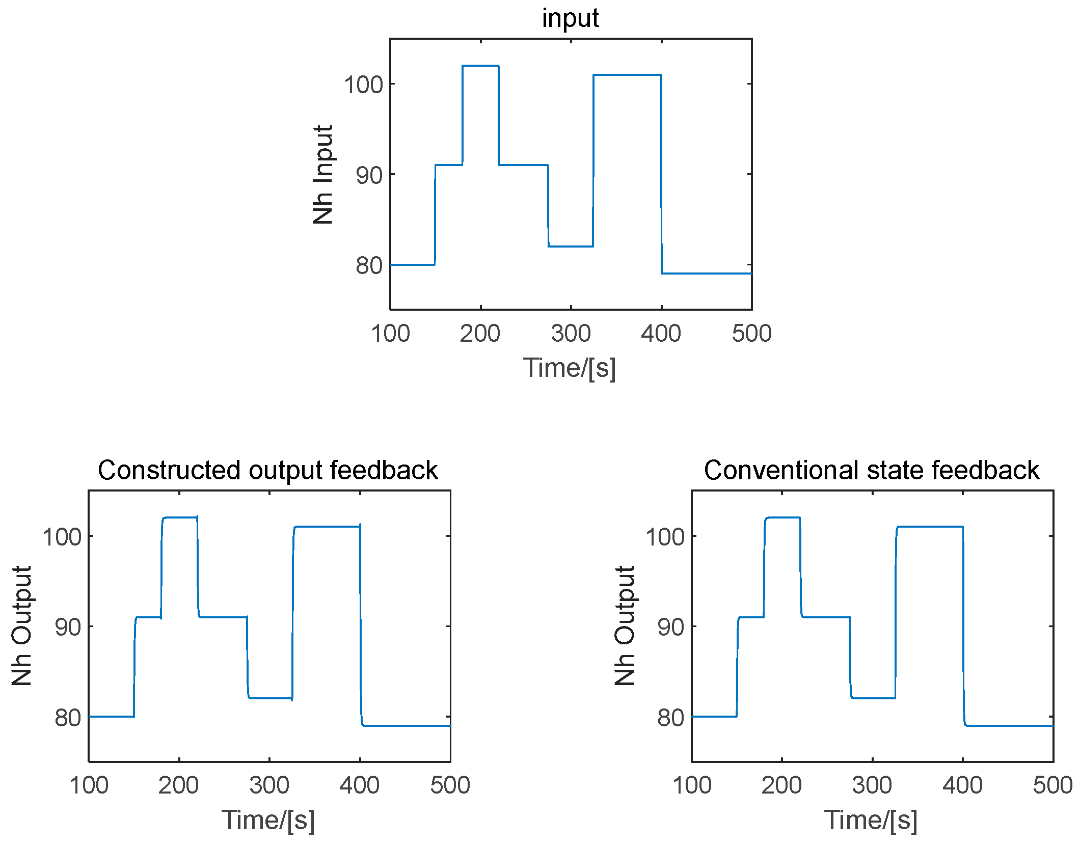
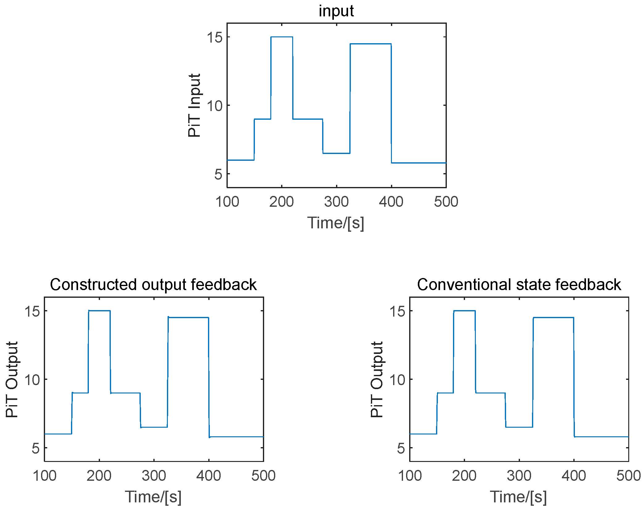
6. Simulation Analyses

From Section 5, we can conclude that the parameter tuning algorithm is simple to calculate, and solving the algorithm process does not involve the complex ARE or Lyapunov equation. It can be calculated with high-reliability low-performance microprocessors.

The VCTs obtained in this paper do not involve complex calculations, making them suitable for meeting the requirements of the SDCS. Additionally, the iterative process of the VCTs’ parameter tuning algorithm also avoids complex calculations. The purposes of the simulation described here are: 1. to verify the convergence rate of the parameter tuning algorithm; and 2. to verify whether the output feedback control constructed in this study achieves equivalent performance to the conventional LQR state feedback control.

Based on the aero-engine model established in Section 2, the analysis in this section includes the following two simulations:

SIMULATION 1.

This simulation focuses on the single-variable aero-engine control. We used the high-pressure rotor speed-control model at the steady point of the relative speed of 83% obtained in Section 2. The eigenvalues of the system matrix of the model are 0.9231 and 0.6576, so it is asymptotically stable. Let $\tilde{Q}=1$, $R=0.49857$, then $Q=\left[1 0;0 0\right]$. The initial feedback gain matrix is $F=\left[\begin{array}{cc}0& 0\end{array}\right]$, and it is calculated that $L_{QR}=\left[1 0 0;0 0 0;0 0 0.49875\right]$. According to the scheme for solving ARE in Equation (41), the optimal feedback gain matrix is $F^{*}=\left[\begin{array}{cc}-0.9120& -0.0252\end{array}\right]$. The convergence details during the iteration are reported in

Table 1. Convergence details of Simulation 1.

$\mathit{\epsilon }$	Steps	$\mathit{F}$	$‖{\mathit{F}}_{\mathit{t}}-{\mathit{F}}_{\mathit{t}+1}‖$	$‖{\mathit{F}}_{\mathit{t}}-{\mathit{F}}^{\mathit{*}}‖$
0.1	3	$\left[\begin{array}{cc}-0.8712& -0.0261\end{array}\right]$	0.0659	0.0274
0.01	4	$\left[\begin{array}{cc}-0.9266& -0.0256\end{array}\right]$	6.0304 × 10−4	0.0140
0.001	4	$\left[\begin{array}{cc}-0.9266& -0.0256\end{array}\right]$	6.0304 × 10−4	0.0140
0.0007	4	$\left[\begin{array}{cc}-0.9266& -0.0256\end{array}\right]$	6.0304 × 10−4	0.0140
0.0006	8	$\left[\begin{array}{cc}-0.9120& -0.0252\end{array}\right]$	3.5857 × 10−5	4.6999 × 10−5

.

The calculation results of $\acute{P}$,$L_{31}$,$L_{32}$,$L_{33}$ are shown in Equation (64), and the parameters of the three VCTs are obtained. Figure 6 shows convergence process of the parameters during the iterative process:

$$\begin{array}{l}\acute{P}=\left[\begin{array}{ccc}3.2878& 0.0530& 0.9692\\ 0.0530& 0.0014& 0.0267\\ 0.9692& 0.0267& 1.0460\end{array}\right]\\ L_{31}=\left[\begin{array}{cc}0.3772& 0.6980\end{array}\right]\\ L_{32}=\left[\begin{array}{cc}-1.2037& 2.0982\end{array}\right]\\ L_{33}=1.4060\end{array}$$

(64)

From Table 1 and Figure 6, the feedback gain matrix $F$ converges rapidly, and $F_t$ converges to $F^{*}$ within eight iterations. The simulation results show that the LQR parameter tuning algorithm proposed in this paper has the characteristics of fewer convergence steps and fast convergence speed. Due to its advantages of simple calculation and rapid convergence, microprocessors with low price, high reliability, and low performance can be utilized for real-time parameter tuning.

The following simulation was conducted to verify the performance of the decentralized LQR output feedback control proposed in this paper. Generally, the performance of optimal state feedback is superior to that of output feedback. Through the design described in Section 4, the LQR output feedback control proposed in this paper can theoretically achieve equivalent performance to the LQR state feedback. This scheme overcomes the shortcomings of state feedback while achieving comparable performance. This simulation compares the LQR output feedback control proposed in this paper with the conventional LQR state feedback control, to validate the aforementioned conclusions.

Figure 7 shows the input and the response curves of the high-pressure rotor speed of the turbofan engine when the output feedback scheme proposed in this paper and the conventional state feedback scheme were adopted, respectively. It can be seen from Figure 7 that the high-pressure rotor speed response curves of the turbofan engine were almost identical when the two schemes were adopted. However, in reality, the two response curves did not completely overlap. As shown in Table 1, this is because there is a certain error between the feedback gain matrices calculated by the primal-dual principle (the output feedback scheme in this paper) and the ARE (the conventional state feedback scheme), respectively. According to the simulation results presented in Figure 7, the output feedback scheme proposed in this paper can achieve equivalent performance to the conventional state feedback, which is consistent with the theoretical analysis in this paper. However, because the state variables of the high-pressure rotor speed model have no physical meaning, the conventional LQR state feedback scheme cannot be used for system design in practical engineering applications. On the other hand, the scheme proposed in this paper can be applied in actual engineering applications, because of the output feedback.

SIMULATION 2.

This simulation focused on the multiple variables of aero-engine control. We used the dual-variable control model of the operating point at a PLA angle of 35°, obtained in Section 2.

The eigenvalues of the system matrix of the model are 0.9644 and 0.9063, so it is asymptotically stable. Let $\tilde{Q}=1$, $R=[1 0;0 1]$, then $Q=\left[1 0;0 1\right]$. The initial feedback gain matrix is $F=\left[0 0;0 0\right]$, and it is calculated that $L_{QR}=\left[1 0 0 0;0 1 0 0;0 0 1 0;0 0 0 1\right]$. According to the scheme for solving ARE in Equation (41), the optimal feedback gain matrix is $F^{*}=\left[-0.0038 0.0017;-7.2976\times {10}^{-4}-0.0010\right]$. The convergence details obtained during the iteration are shown in

Table 2. Convergence details of Simulation 2.

$\mathit{\epsilon }$	Steps	$\mathit{F}$	$‖{\mathit{F}}_{\mathit{t}}-{\mathit{F}}_{\mathit{t}+1}‖$	$‖{\mathit{F}}_{\mathit{t}}-{\mathit{F}}^{\mathit{*}}‖$
0.1	1	$\left[\begin{array}{cc}-0.0038& 0.0017\\ -7.2977\times {10}^{-4}& -0.001\end{array}\right]$	0.0041	0.0041
0.01	1	$\left[\begin{array}{cc}-0.0038& 0.0017\\ -7.2977\times {10}^{-4}& -0.001\end{array}\right]$	0.0041	0.0042
0.001	2	$\left[\begin{array}{cc}-0.0038& 0.0017\\ -7.2976\times {10}^{-4}& -0.001\end{array}\right]$	4.8053 × 10−9	6.9260 × 10−8
0.0001	2	$\left[\begin{array}{cc}-0.0038& 0.0017\\ -7.2976\times {10}^{-4}& -0.001\end{array}\right]$	4.8053 × 10−9	4.1779 × 10−5
4.0 × 10−9	5	$\left[\begin{array}{cc}-0.0038& 0.0017\\ -7.2976\times {10}^{-4}& -0.001\end{array}\right]$	3.8062 × 10−9	5.6807 × 10−8

.

The calculation result of $\acute{P}$, $L_{31}$, $L_{32}$, $L_{33}$ is shown in Equation (65), and the parameters of the three VCTs were obtained. The convergence of the parameters during the iterative process is shown in Figure 8.

$$\begin{array}{l}\acute{P}=\left[\begin{array}{cccc}13.5543& -7.2729& 0.0038& 7.2976\times {10}^{-4}\\ -7.2729& 11.3840& -0.0017& 0.0010\\ 0.0038& -0.0017& 1.0& 3.4001\times {10}^{-7}\\ 7.2976\times {10}^{-4}& 0.0010& 3.4001\times {10}^{-7}& 1.0\end{array}\right]\\ L_{31}=1.0\times {10}^{-5}\times \left[\begin{array}{cccc}0.0545& 0.0123& 0.1123& 0.0288\\ 0.0162& 0.0166& 0.0317& 0.0334\end{array}\right]\\ L_{32}=\left[\begin{array}{cccc}0.0018& -0.0009& 0.0018& -0.0009\\ 0.0004& 0.0004& 0.0003& 0.0004\end{array}\right]\\ L_{33}=\left[\begin{array}{cc}1.0& 0.0\\ 0.0& 1.0\end{array}\right]\end{array}$$

(65)

As shown in Table 2 and Figure 8, the feedback gain matrix $F$ converged rapidly, and $F_t$ converged to $F^{*}$ within five iterations. In fact, only one or two iterations were needed to obtain a feedback gain matrix $F$ with sufficient accuracy. The simulation results show that the LQR parameter tuning algorithm proposed in this paper has the characteristics of fewer convergence steps and fast convergence speed. Due to its advantages of simple calculation and rapid convergence, microprocessors with low price, high reliability, and low performance can be utilized for real-time parameter tuning.

Figure 9 shows the input and the response curves of the high-pressure rotor speed of the turbofan engine when the output feedback scheme and the conventional state feedback scheme were adopted, respectively. Figure 10 shows the input and the response curves of the pressure ratio when the two feedback schemes were adopted, respectively. It can be seen from Figure 9 that the high-pressure rotor speed response curves of the turbofan engine were almost identical when the two schemes were adopted, and the same applies for the pressure ratio response curves in Figure 10. However, in both Figure 9 and Figure 10, the system response of the two feedback schemes do not completely overlap. This is because there is a certain error between the feedback gain matrices calculated by the primal-dual principle and the ARE. According to the simulation results presented in Figure 9 and Figure 10, the output feedback scheme proposed in this paper can achieve equivalent performance to conventional state feedback, which is consistent with the theoretical analysis in this paper. However, because the state variables of the dual-variable control model have no physical meaning, the conventional LQR state feedback scheme cannot be used for system design in practical engineering applications. On the other hand, the scheme proposed in this paper can be applied in actual engineering applications because of the output feedback.

According to the results of Simulations 1 and 2, the constructed output feedback scheme can achieve performance equivalent to that of the state feedback scheme. Furthermore, the proposed parameter tuning algorithm exhibits fast convergence speed and high accuracy. These simulation results show the effectiveness of the design scheme presented in this paper.

7. Conclusions

We propose a decentralized design scheme for controllers of aero-engines, the SDCS. In SDCS, a group of low-price, high-reliability, but low-performance microprocessors act as the controller of the aero-engine control system. An output feedback scheme based on Q-Learning LQR is constructed, and the VCTs of the SDCS are obtained. The constructed output feedback scheme is equivalent to the optimal state feedback control. A controller parameter tuning algorithm based on the primal-dual principle is introduced, which features simple calculation and can be implemented using low-cost, high-reliability, low-performance microprocessors for real-time calculation, suitable for the hardware characteristics of SDCS. Finally, we conducted simulation for verification. According to the simulation results, the controller parameter tuning algorithm proposed in this paper converges quickly and has high convergence accuracy. The single-variable model takes only a maximum of eight iterations to obtain a high-precision feedback gain matrix, and the multi-variable model takes a maximum of only five iterations. In addition, the constructed output feedback scheme achieves control performance equivalent to the conventional state feedback, which is suitable for the actual engineering application of the aero-engine control system. The simulation results demonstrate the effectiveness of the design scheme presented in this paper.

References

1. Thompson, H.; Fleming, P. Distributed Aero-Engine Control Systems Architecture Selection Using Multi-Objective Optimisation. In Proceedings of the 5th IFAC Workshop on Algorithms & Architecture for Real Time Control (AARTC’ 98), Cancun, Mexico, 15–17 April 1998. [Google Scholar]
2. Skira, C.; Agnello, M. Control Systems for the Next Century’s Fighter Engines. J. Eng. Gas Turbines Power 1992, 114, 749–754. [Google Scholar] [CrossRef]
3. Culley, D.; Thomas, R.; Saus, J. Concepts for Distributed Engine Control. In Proceedings of the 43rd AIAA/ASME/SAE/ASEE Joint Propulsion Conference & Exhibit, Cincinnati, OH, USA, 8–11 July 2007. [Google Scholar]
4. Chen, T.; Shan, J. Distributed Tracking of Multiple Under-actuated Lagrangian Systems with Uncertain Parameters and Actuator Faults. In Proceedings of the 2019 American Control Conference (ACC), Philadelphia, PA, USA, 10–12 July 2019. [Google Scholar]
5. Chen, T.; Shan, J. Distributed Tracking of a Class of Underactuated Lagrangian Systems with Uncertain Parameters and Actuator Faults. IEEE Trans. Ind. Electron. 2020, 67, 4244–4253. [Google Scholar] [CrossRef]
6. Chen, T.; Shan, J. Distributed Fixed-time Control of Multi-agent Systems with Input Shaping. In Proceedings of the 2018 IEEE International Conference on Information and Automation (ICIA), Wuyishan, China, 11–13 August 2018. [Google Scholar]
7. Chen, T.; Shan, J. Distributed Adaptive Attitude Control for Multiple Underactuated Flexible Spacecraft. In Proceedings of the 2018 Annual American Control Conference (ACC), Milwaukee, WI, USA, 27–29 June 2018. [Google Scholar]
8. Thompson, H.; Benitez-Perez, H.; Lee, D.; Ramos-Hernandez, D.; Fleming, P.; Legge, C. A CANbus-Based Safety-Critical Distributed Aeroengine Control Systems Architecture Demonstrator. Microprocess. Microsyst. 1999, 23, 345–355. [Google Scholar] [CrossRef]
9. Chen, L.; Guo, Y. Design of the Distributed Control System Based on CAN Bus. Comput. Inf. Sci. 2011, 4, 83–89. [Google Scholar] [CrossRef]
10. Lv, C.; Chang, J.; Bao, W.; Yu, D. Recent Research Progress on Airbreathing Aero-engine Control Algorithm. Propuls. Power Res. 2022, 11, 1–57. [Google Scholar] [CrossRef]
11. Xu, Y.; Pan, M.; Huang, J.; Zhou, W.; Qiu, X.; Chen, Y. Estimation-Based and Dropout-Dependent Control Design for Aeroengine Distributed Control System with Packet Dropout. Int. J. Aerosp. Eng. 2022, 2022, 8658704. [Google Scholar] [CrossRef]
12. Fan, X.; Pan, M.; Huang, J. Response Time Analysis of TTCAN Bus for Aero-engine Distributed Control System. In Proceedings of the Asia-Pacific International Symposium on Aerospace Technology (APISAT 2015), Cairns, QLD, Australia, 25–27 November 2015. [Google Scholar]
13. Schley, W. Distributed Flight Control and Propulsion Control Implementation Issues and Lessons Learned. In Proceedings of the ASME 1998 International Gas Turbine and Aeroengine Congress and Exhibition, Stockholm, Sweden, 2–5 June 1998. [Google Scholar]
14. Zulkifli, N.; Ramli, M. State Feedback Controller Tuning for Liquid Slosh Suppression System Utilizing LQR-LMI Approach. In Proceedings of the 2021 IEEE International Conference on Automatic Control & Intelligent Systems (I2CACIS), Shah Alam, Malaysia, 26–26 June 2021. [Google Scholar]
15. Zhou, Y.; Xu, G.; Wei, S.; Zhang, X.; Huang, Y. Experiment Study on the Control Method of Motor-Generator Pair System. IEEE Access 2017, 6, 925–936. [Google Scholar] [CrossRef]
16. Wu, A.; Qian, Y.; Liu, W.; Sreeram, V. Linear Quadratic Regulation for Discrete-Time Antilinear Systems: An Anti-Riccati Matrix Equation Approach. J. Frankl. Inst. 2016, 353, 1041–1060. [Google Scholar] [CrossRef]
17. Bhawal, C.; Qais, I.; Pal, D. Constrained Generalized Continuous Algebraic Riccati Equation (CGCAREs) Are Generically Unsolvable. IEEE Control Syst. Lett. 2019, 3, 192–197. [Google Scholar] [CrossRef]
18. Rizvi, S.; Lin, Z. Output Feedback Optimal Tracking Control Using Reinforcement Q-Learning. In Proceedings of the 2018 Annual American Control Conference (ACC), Milwaukee, WI, USA, 27–29 June 2018. [Google Scholar]
19. Lewis, F.; Vamvoudakis, K. Reinforcement Learning for Partially Observable Dynamic Processes: Adaptive Dynamic Programming Using Measured Output Data. IEEE Trans. Syst. Man Cybern. Part B 2011, 41, 14–25. [Google Scholar] [CrossRef] [PubMed]
20. Salhi, S.; Salhi, S. LQR Control of a Grid Side Converter of a DFIG Based WECS: LMI Approach Based on Lyapunov Condition. In Proceedings of the 2019 16th International Multi-Conference on Systems, Signals & Devices (SSD), Istanbul, Turkey, 21–24 March 2019. [Google Scholar]
21. Nguyen, T.; Gajic, Z. Solving the Matrix Differential Riccati Equation: A Lyapunov Equation Approach. IEEE Trans. Autom. Control 2010, 55, 191–194. [Google Scholar]
22. Bi, H.; Chen, D. The Estimation of the Solutions Matrix of the Perturbed Discrete Time Algebraic Riccati Equation. In Proceedings of the 10th World Congress on Intelligent Control and Automation, Beijing, China, 6–8 July 2012. [Google Scholar]
23. Vargas, F.; Gonzalez, R. On the Existence of a Stabilizing Solution of Modified Algebraic Riccati Equations in Terms of Standard Algebraic Riccati Equations and Linear Matrix Inequalities. IEEE Control Syst. Lett. 2020, 4, 91–96. [Google Scholar] [CrossRef]
24. Chen, M.; Zhang, L.; Su, H.; Chen, G. Stabilizing Solution and Parameter Dependence of Modified Algebraic Riccati Equation with Application to Discrete-Time Network Synchronization. IEEE Trans. Autom. Control 2016, 61, 228–233. [Google Scholar] [CrossRef] [Green Version]
25. Chapman, J.; Litt, J. Control Design for an Advanced Geared Turbofan Engine. In Proceedings of the 53rd AIAA/SAE/ASEE Joint Propulsion Conference, Atlanta, GA, USA, 10–12 July 2017. [Google Scholar]
26. Mawid, M.; Park, T.; Sekar, B.; Arana, C. Application of Pulse Detonation Combustion to Turbofan Engines. J. Eng. Gas Turbines Power 2003, 125, 270–283. [Google Scholar] [CrossRef]
27. Pavlenko, D.; Dvirnyk, Y.; Przysowa, R. Advanced Materials and Technologies for Compressor Blades of Small Turbofan Engine. Aerospace 2021, 8, 1. [Google Scholar] [CrossRef]
28. Gharoun, H.; Keramati, A.; Nasiri, M. An Integrated Approach for Aircraft Turbofan Engine Fault Detection Based on Data Mining Techniques. Expert Syst. 2019, 36, e12370. [Google Scholar] [CrossRef]
29. Li, J. Turbofan Engine H Output Feedback Control and Delay Compensation Strategy. Master’s Thesis, Dalian University of Technology, Dalian, China, 2021. [Google Scholar]
30. Belapurkar, R. Stability and Performance of Propulsion Control Systems with Distributed Control Architectures and Failures. Ph.D. Thesis, The Ohio State University, Columbus, OH, USA, 2012. [Google Scholar]
31. Balakrishnan, V.; Vandenberghe, L. Semidefinite Programming Duality and Linear Time-Invariant Systems. IEEE Trans. Autom. Control 2003, 48, 30–41. [Google Scholar] [CrossRef] [Green Version]
32. Gattami, A. Generalized Linear Quadratic Control. IEEE Trans. Autom. Control 2010, 55, 131–136. [Google Scholar] [CrossRef]
33. Lee, D.; Hu, J.H. Primal-Dual Q-Learning Framework for LQR Design. IEEE Trans. Autom. Control 2019, 64, 3756–3763. [Google Scholar] [CrossRef]
Figure 1. Schematic diagram of a turbofan engine.
Actuators 12 00164 g001
Figure 2. Overview of a traditional aero-engine DCS.
Actuators 12 00164 g002
Figure 3. Overview of the decentralized controller.
Actuators 12 00164 g003
Figure 4. Output feedback control.
Actuators 12 00164 g004
Figure 5. The networks acts as the output feedback controller.
Actuators 12 00164 g005
Figure 6. Convergence trajectory of F t F t + 1 and F t F * during the iterative process.
Actuators 12 00164 g006
Figure 7. High-pressure rotor speed response curve.
Actuators 12 00164 g007
Figure 8. Convergence trajectory of F t F t + 1 and F t F * during the iterative process.
Actuators 12 00164 g008
Figure 9. High-pressure rotor speed response curve.
Actuators 12 00164 g009
Figure 10. Pressure ratio response curve.
Actuators 12 00164 g010