
Non-Reciprocal MEMS Periodic Structure


Abstract
1. Introduction
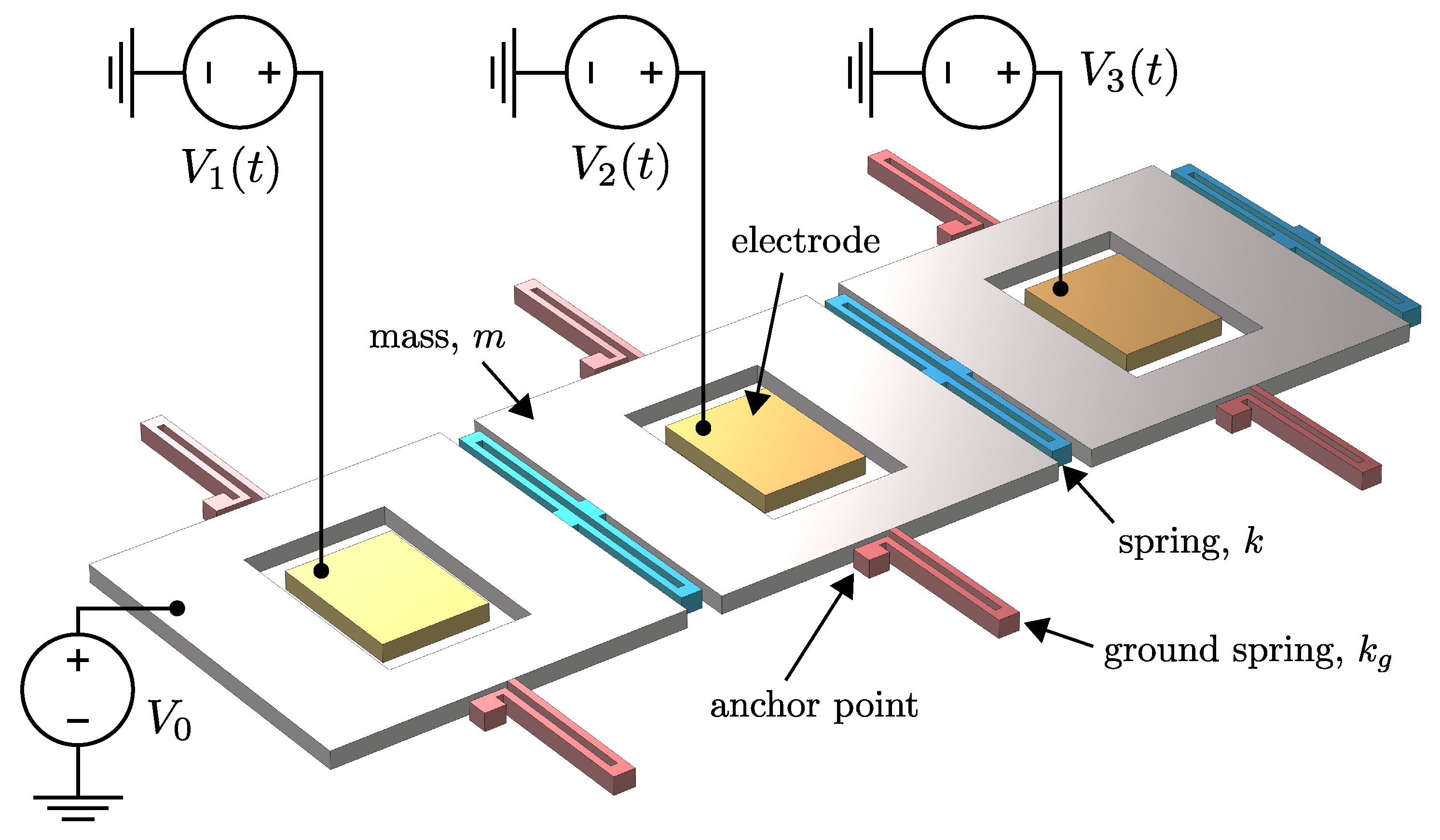
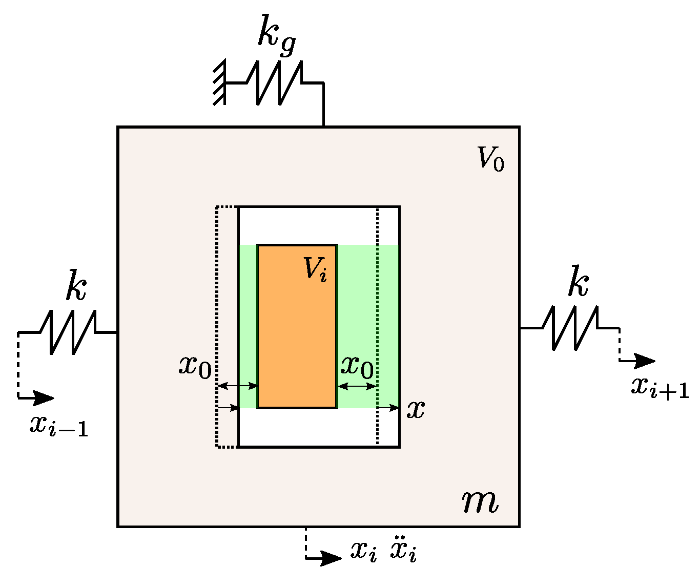
2. The Model
3. Parametric Analysis for Harmonic Modulation
3.1. Dispersion Relation for Rod on Elastic Foundations
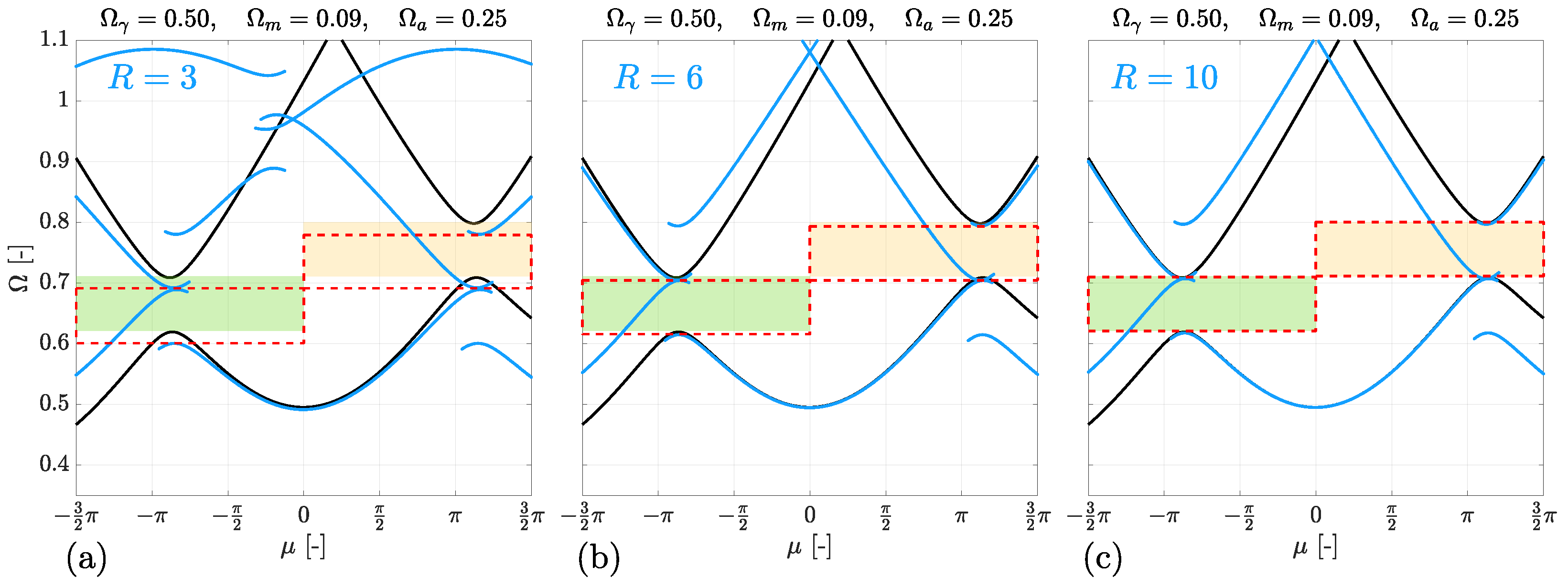
3.2. Dispersion Analysis
3.3. From Rod to Spring-Mass Chain
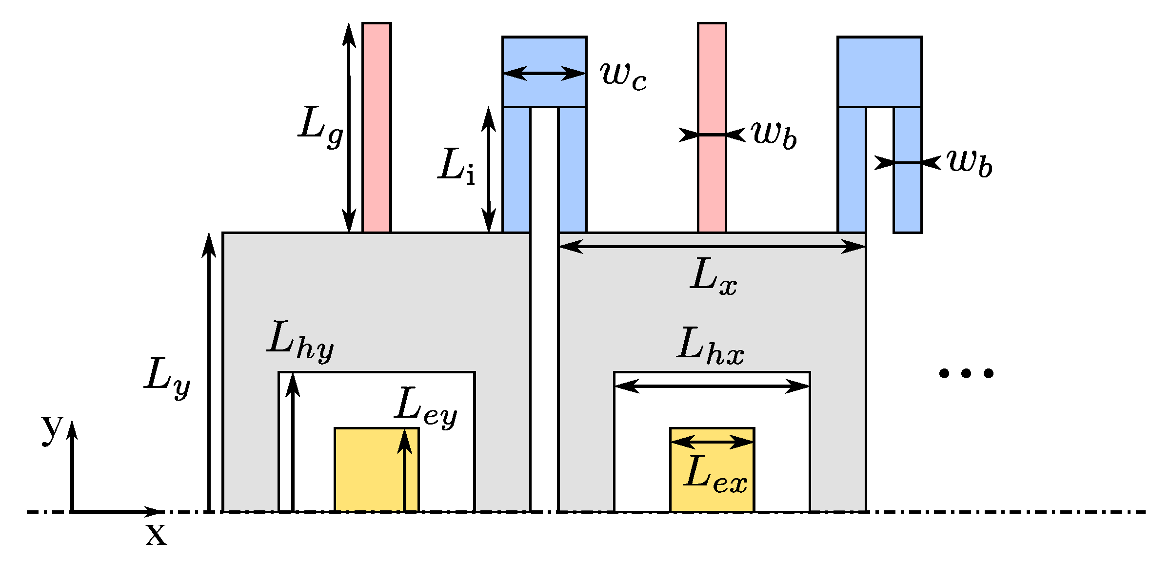
4. Numerical Study of the MEMS Device
5. Conclusions
Author Contributions
Funding
Data Availability Statement
Conflicts of Interest
References
- Hussein, M.I.; Leamy, M.J.; Ruzzene, M. Dynamics of phononic materials and structures: Historical origins, recent progress, and future outlook. Appl. Mech. Rev. 2014, 66, 040802. [Google Scholar] [CrossRef]
- Kadic, M.; Milton, G.W.; van Hecke, M.; Wegener, M. 3D metamaterials. Nat. Rev. Phys. 2019, 1, 198–210. [Google Scholar] [CrossRef]
- Trainiti, G.; Xia, Y.; Marconi, J.; Cazzulani, G.; Erturk, A.; Ruzzene, M. Time-periodic stiffness modulation in elastic metamaterials for selective wave filtering: Theory and experiment. Phys. Rev. Lett. 2019, 122, 124301. [Google Scholar] [CrossRef] [PubMed]
- Xia, Y.; Riva, E.; Rosa, M.I.; Cazzulani, G.; Erturk, A.; Braghin, F.; Ruzzene, M. Experimental observation of temporal pumping in electromechanical waveguides. Phys. Rev. Lett. 2021, 126, 095501. [Google Scholar] [CrossRef] [PubMed]
- Trainiti, G.; Ruzzene, M. Non-reciprocal elastic wave propagation in spatiotemporal periodic structures. New J. Phys. 2016, 18, 083047. [Google Scholar] [CrossRef]
- Vila, J.; Pal, R.K.; Ruzzene, M.; Trainiti, G. A bloch-based procedure for dispersion analysis of lattices with periodic time-varying properties. J. Sound Vib. 2017, 406, 363–377. [Google Scholar] [CrossRef]
- Marconi, J.; Riva, E.; Di Ronco, M.; Cazzulani, G.; Braghin, F.; Ruzzene, M. Experimental observation of nonreciprocal band gaps in a space-time-modulated beam using a shunted piezoelectric array. Phys. Rev. Appl. 2020, 13, 031001. [Google Scholar] [CrossRef]
- Chen, Y.; Li, X.; Nassar, H.; Norris, A.N.; Daraio, C.; Huang, G. Nonreciprocal wave propagation in a continuum-based metamaterial with space-time modulated resonators. Phys. Rev. Appl. 2019, 11, 064052. [Google Scholar] [CrossRef]
- Nassar, H.; Yousefzadeh, B.; Fleury, R.; Ruzzene, M.; Alù, A.; Daraio, C.; Norris, A.N.; Huang, G.; Haberman, M.R. Nonreciprocity in acoustic and elastic materials. Nat. Rev. Mater. 2020, 5, 667–685. [Google Scholar] [CrossRef]
- Yu, Y.; Michetti, G.; Pirro, M.; Kord, A.; Sounas, D.L.; Xiao, Z.; Cassella, C.; Alu, A.; Rinaldi, M. Radio Frequency Magnet-Free Circulators Based on Spatiotemporal Modulation of Surface Acoustic Wave Filters. IEEE Trans. Microw. Theory Technol. 2019, 67, 4773–4782. [Google Scholar] [CrossRef]
- Ashley, A.; Psychogiou, D. RF Co-Designed Bandpass Filters/Isolators Using Nonreciprocal Resonant Stages and Microwave Resonators. IEEE Trans. Microw. Theory Technol. 2021, 69, 2178–2190. [Google Scholar] [CrossRef]
- Weinstein, D.; Bhave, S.A.; Tada, M.; Mitarai, S.; Morita, S.; Ikeda, K. Mechanical coupling of 2D resonator arrays for MEMS filter applications. In Proceedings of the 2007 IEEE International Frequency Control Symposium Joint with the 21st European Frequency and Time Forum, Geneva, Switzerland, 29 May–1 June 2007; IEEE: Piscataway, NJ, USA, 2007; pp. 1362–1365. [Google Scholar]
- Pirro, M.; Cassella, C.; Michetti, G.; Chen, G.; Kulik, P.; Yu, Y.; Rinaldi, M. Novel topology for a non-reciprocal MEMS filter. In Proceedings of the 2018 IEEE International Ultrasonics Symposium (IUS), Kobe, Japan, 22–25 October 2018; IEEE: Piscataway, NJ, USA, 2018; pp. 1–3. [Google Scholar]
- Yu, Y.; Michetti, G.; Kord, A.; Sounas, D.; Pop, F.V.; Kulik, P.; Pirro, M.; Qian, Z.; Alu, A.; Rinaldi, M. Magnetic-free radio frequency circulator based on spatiotemporal commutation of MEMS resonators. In Proceedings of the 2018 IEEE Micro Electro Mechanical Systems (MEMS), Belfast, UK, NJ, USA, 21–25 January 2018; IEEE: Piscataway, NJ, USA, 2018; pp. 154–157. [Google Scholar]
- Acar, C.; Shkel, A. MEMS Vibratory Gyroscopes: Structural Approaches to Improve Robustness; Springer: Berlin/Heidelberg, Germany, 2008. [Google Scholar]
- Marconi, J.; Cazzulani, G.; Riva, E.; Braghin, F. Observations on the behavior of discretely modulated spatiotemporal periodic structures. In Proceedings of the Active and Passive Smart Structures and Integrated Systems XII, Denver, CO, USA, 5–8 March 2018; Erturk, A., Ed.; International Society for Optics and Photonics, SPIE: Cergy-Pontoise, France, 2018; Volume 10595, pp. 630–636. [Google Scholar] [CrossRef]
- Riva, E.; Marconi, J.; Cazzulani, G.; Braghin, F. Generalized plane wave expansion method for non-reciprocal discretely modulated waveguides. J. Sound Vib. 2019, 449, 172–181. [Google Scholar] [CrossRef]


| [GPa] | silicon elastic modulus |
| [kg/m] | silicon density |
| [m] | silicon wafer thickness |
| [m] | cell spatial period |
| [F/m] | vacuum permittivity |
| [V] | AC voltage amplitude |
| [V] | DC voltage amplitude |
| [rad/s] | voltage modulation frequency |
| [N/m] | stiffness between masses |
| [N/m] | ground stiffness |
| [N/m] | constant electrostatic stiffness |
| [N/m] | time-modulated electrostatic stiffness |
| [ng] | mass value |
Disclaimer/Publisher’s Note: The statements, opinions and data contained in all publications are solely those of the individual author(s) and contributor(s) and not of MDPI and/or the editor(s). MDPI and/or the editor(s) disclaim responsibility for any injury to people or property resulting from any ideas, methods, instructions or products referred to in the content. |
© 2023 by the authors. Licensee MDPI, Basel, Switzerland. This article is an open access article distributed under the terms and conditions of the Creative Commons Attribution (CC BY) license (https://creativecommons.org/licenses/by/4.0/).
Share and Cite
Marconi, J.; Enrico Quadrelli, D.; Braghin, F. Non-Reciprocal MEMS Periodic Structure. Actuators 2023, 12, 161. https://doi.org/10.3390/act12040161
Marconi J, Enrico Quadrelli D, Braghin F. Non-Reciprocal MEMS Periodic Structure. Actuators. 2023; 12(4):161. https://doi.org/10.3390/act12040161
Chicago/Turabian StyleMarconi, Jacopo, Davide Enrico Quadrelli, and Francesco Braghin. 2023. "Non-Reciprocal MEMS Periodic Structure" Actuators 12, no. 4: 161. https://doi.org/10.3390/act12040161
APA StyleMarconi, J., Enrico Quadrelli, D., & Braghin, F. (2023). Non-Reciprocal MEMS Periodic Structure. Actuators, 12(4), 161. https://doi.org/10.3390/act12040161