Abstract
In this paper, a new nonlinear robust fault-tolerant tracking control method is proposed for a tri-rotor unmanned aerial vehicle (UAV) under unknown abnormal actuator behaviors together with unknown external disturbances. The actuator anomalies are modeled as time-varying multiplicative parameters to improve the model accuracy. The control system is decoupled into two parts, including the inner-loop attitude control and the outer-loop position control. The radial basis function neural network (RBFNN) is utilized in the outer loop to estimate the actuator anomalies and external disturbances, and then the state feedback controller is employed for the position tracking of the UAV. Then, the robust integral of the signum of the error (RISE) controller is designed for the inner loop to compensate for actuator anomalies and external disturbances. The composite stability of the closed-loop system and the asymptotical tracking performance are proved via a Lyapunov-based stability analysis. Numerical simulations based on the proposed fault tolerant control (FTC) scheme as well as the comparison results with a sliding mode-based FTC method validate the effectiveness and better performance of the proposed control design.
1. Introduction
In recent years, the multi-rotor unmanned aerial vehicle (UAV) has attracted increasing attention for both military and civil applications, such as fire surveillance, agricultural survey, and so on [1,2]. Different from other multi-rotor UAVs, the tri-rotor UAV shows some unique advantages, such as a simpler structure, lower cost, lower energy consumption, and higher maneuverability [3,4]. The mechanical structure of a tri-rotor UAV consists of two fixed motors and one tilt motor equipped on a rear servo [5]. Therefore, the movement of the tri-rotor UAV is generated by the rotation of the three motors and deflection of the tilt rear servo, which are the so-called actuators [6]. Meanwhile, with the development of the tri-rotor UAV, the frequent occurrence of abnormal behaviors of the UAV has been inevitable [7]. In fact, with the continuous operation of the actuators, the risk of anomalies from the actuators anomalies is greatly increased; thus, the tri-rotor UAV could become unstable or even out of control, which makes the fault-tolerant control (FTC) of the tri-rotor UAV significant [8]. As we all know, the tri-rotor UAV has six DOFs with only four inputs, which is a typical underactuated system and which therefore makes the situation more serious when anomalies of the actuators happen [9]. Most existing works are mainly focused on the dynamic modeling and flight control of tri-rotor UAVs. In [10], a dynamic model of a tri-rotor UAV was obtained via the Newton–Euler approach, and then the saturating-function-based sequential control strategy was utilized to realize the position tracking control, which was verified through real-time experiments on a self-built Simulink-based platform. In [11], a PID-based attitude control and a linear quadratic translational control for a tri-rotor UAV was presented, and numerical simulation results demonstrated its efficiency. In [12], an adaptive hybrid scheme was utilized for the attitude and altitude control of a tri-rotor UAV. The numerical simulation results showed a better transient response with a low overshoot and undershoot to achieve the desired attitude. What can be concluded from the above is that studies on tri-rotor UAVs mainly focus on dynamic modeling and flight control, which have been validated by numerical simulations or real-time experiments, while quite few studies have taken the FTC of tri-rotor UAVs into consideration.
Apart from tri-rotor UAVs, studies of the FTC of other types of multi-rotor UAVs, such as quadrotor UAVs and hexacopter UAVs, may also bring us inspiration. For the FTC of quadrotor UAVs and hex-rotor UAVs, algorithms such as PID control [13], adaptive control [14], sliding mode control [15], and robust control [16] have been utilized [17,18]. In [19], a data-driven fault-tolerant synchronization control scheme based on a distributed observer and optimal control policy was investigated for unknown cooperative quadrotors subject to nonlinearities and multiple actuator anomalies in the quadrotor dynamics. In [20], two FTC designs based on gain-scheduling control were presented for a multi-copter UAV subject to actuator anomalies. In [21], the authors surveyed the trajectory tracking issue of underactuated vertical takeoff and landing UAVs subject to a loss of efficiency and actuator biases. In [22], an active FTC strategy was proposed for time-varying actuator anomalies, and the time-delay phenomenon caused by fault diagnosis was discussed. In [23], an adaptive FTC allocation method was presented to solve the trajectory tracking problem of a hexacopter UAV against degradation and failures of the propulsion system without accurate fault information and online optimization. The effectiveness of the proposed FTC strategies were verified through real-time flght experiments, and the control performances were analyzed quantitatively.
In our previous work [24,25], nonlinear FTC laws wee designed to maintain the stability of a tri-rotor UAV under an unknown rear servo’s stuck fault, and real-time experiments validated the robust performance. To further address our research, an inner-outer-loop-based fault-tolerant tracking control strategy is developed for the tri-rotor UAV, and the main contributions of this article can be summarized as follows. First, the actuator anomalies of the tri-rotor UAV are taken into consideration, while most existing works do not consider this issue, which is modeled as some time-varying multiplicative parameters to improve the model accuracy. Second, the control system is decoupled into the inner-loop attitude control and outer-loop position control. For the outer loop, approximation components based on RBFNN are introduced to estimate the unknown external disturbances and actuator anomalies, and then the state feedback algorithm is employed to design the position controller [26,27]. For the inner loop, a RISE-based controller is developed to compensate for the unknown exogenous disturbances together with actuator anomalies without an additional fault isolation and reconstruction mechanism [28]. Third, the composite stability of the cascaded system is proved by Lyapunov theory. Finally, numerical simulations and the comparison with sliding mode (SM) methodology are provided to illustrate the better tracking performance of the proposed FTC strategy. To our best knowledge, few existing works have taken the FTC of tri-rotor UAV into consideration, and the control methods proposed in this article also have not been utilized in the control of a tri-rotor UAV.
This paper is organized as follows. The dynamics of the tri-rotor UAV under actuator anomalies are described in Section 1. In Section 2 and Section 3, the design of the FTC scheme and the composite stability analysis are presented. Numerical simulation results are shown in Section 4. Finally, some conclusion remarks are included in Section 5.
2. Problem Formulation
In order to describe the dynamics and kinematics of a tri-rotor UAV, two right-hand coordinate systems are utilized. One is the inertial frame represented by , the origin of which is attached on the ground, with being the vertical direction downward into the ground, being the east direction, and being determined by the right-hand rule. The other one is the body-fixed frame represented by which is centered at the centroid of the tri-rotor UAV. The body axis is the normal axis of the principal plane of the tri-rotor UAV directed from top to bottom, the body axis is along with the backward flying direction of the tri-rotor, and the direction of the body axis is determined by the right-hand rule, as illustrated in Figure 1.
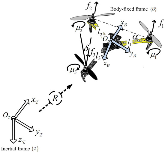
Figure 1.
Schematic of tri-rotor UAV.
In Figure 1, motor 1 and motor 2 rotate clockwise, and motor 3 rotates anti-clockwise. Meanwhile, the relationship between the rotational torques and the thrust force generated by the three motors can be illustrated via the following equation,
where the symbols and denote the total thrust force and rotational torques produced by the three motors and the rear servo, and the symbols and represent the thrust and anti-torque produced by the ith motor, respectively. The constant denotes the distance between the ith motor and the origin . Supposing there was a line connecting motor 1 to motor 2 and another connecting motor 1 to the origin , then an angle would be formulated between these two lines, which is denoted by . The signal represents the angle by which the rear servo deviates from the plane of , with clockwise being the positive direction.
For the convenience of the subsequent control development, the following assumptions are proposed.
Assumption 1.
The structure of the tri-rotor UAV is symmetrical with respect to the axis of , so the equation of is established, where l is a constant.
Assumption 2.
The terms of are neglected, and equals to 1 since the angle varies within a quite small range. Actually, the normal variation range of the angle is bounded within
When Assumptions 1 and 2 are all satisfied(1) and can be rewritten as follows:
The Euclidean position and Euler angle of the UAV with respect to the frame are represented by and , and then the dynamic model of the tri-rotor UAV expressed in is given in the following form [29]:
where denotes the mass of the UAV, is a positive definite inertial matrix, is the Coriolis and centrifugal matrix, g is the acceleration of the gravity, and and are the rotation matrixes expressed as follows,
where s and c are abbreviations for and In (3), and represent the unknown external disturbances.
Because of the singularity of the tri-rotor UAV system at the following assumption is presented.
Assumption 3.
The UAV’s pitch angle satisfies
For the convenience of the subsequent control development, the dynamic model of the tri-rotor UAV in (3) can be rewritten as
When the actuator anomalies occur in the tri-rotor UAV, the total thrust force and rotational torque will be decreased to some extent. Then, the fault dynamics of the tri-rotor UAV can be obtained as follows.
where , and different values of the parameter means different actuator anomalies, which are listed as follows:
Assumption 4.
From the above, we know that , the total thrust and rotational torques are bounded, i.e., , and therefore, where , , , are some unknown bounded constants.
Remark 1.
The overall control object is to design the total thrust and rotational torques to ensure the tri-rotor UAV track’s time-varying trajectories under actuator anomalies.
3. Control Development
Let be the desired position, and then the position tracking error and the filtered error are obtained as
After taking the time derivative of (12) and substituting (6) together with (11) into the resulting equation, the position error dynamics can be obtained as
The dynamics described in (6) can be considered a cascaded structure where the position and attitude subsystem are coupled through the rotation matrix . Hence, to formulate the problem as the control of two connected systems, a virtual control vector defined as is introduced.
Then, the open-loop system can be obtained after introducing and substituting (6) into (13),
where is the desired attitude and is obtained as
Similar to the above analysis, the attitude tracking error and the filtered error are obtained as
After taking the time derivative of (19) and substituting (6) together with (18) into the resulting equation, the attitude error dynamics can be obtained as
For the system in cascade, one of the most important theorems on its stability analysis is the following theorem expressed in [30].
Theorem 1.
If there is a feedback such that is an asymptotically stable equilibrium of , then any partial state feedback control , which renders the -subsystem equilibrium asymptotically stable, also achieves the asymptotic stability of .
From Theorem 1 and also according to references [29,31], the main control development can be achieved in the following three steps.
- 1.
- Choose the control law for the system of without the interconnection term to ensure the tracking error converges to 0 asymptotically.
- 2.
- Choose the control law for the system of to ensure the tracking error converges to 0 asymptotically.
- 3.
- Prove that and converge to 0 asymptotically considering the coupling term .
3.1. Outer-Loop Position Controller Design Based on RBFNN State Feedback Method
For the outer-loop system the objective is to design the auxiliary control input to ensure that the tracking error converges to zero asymptotically.
For the unknown continuous term of , we utilize RBFNN to approximate them over the compact set Then, can be re-expressed in the following form:
where is the ideal weight with the neuron number q, is the basis function vectors with is the center of receptive field, , and is the approximation error. Since the ideal weight matrix is an unknown constant matrix, which is unavailable for the actual control design, we introduce the estimation of the ideal RBFNN weight represented by , which satisfies
and the control input can be expressed as
where is a positive constant matrix.
Theorem 2.
Proof of Theorem 2.
Define the Lyapunov candidate function as
After taking the time derivative of (26) and substituting (24) together with (22) into the resulting equation, the following expression can be obtained:
Let then the following inequality is obtained as
where c is a positive constant. Then,
where
After solving the inequality (29), the following inequality is obtained:
From the above inequality, it can be proven that (i) these errors , are semiglobally uniformly ultimately bounded (SGUUB); (ii) the filtered error is exponentially stable when choosing large enough design parameters; (iii) according to (12), the tracking error is also exponentially stable, which is stronger than asymptotical stability. □
After the above analysis, for the outer-loop position control, the RBFNN is utilized to estimate the actuator anomalies and external disturbances, and then the state feedback controller is employed for the position tracking control of the UAV.
3.2. Inner-Loop Attitude Controller Design Based on RISE Method
For the system the objective is to design the control scheme to ensure the asymptotic convergence of the tracking error in (18). Before presenting the control law, some auxiliary error signals are defined first. The new filtered signal is denoted by is calculated as
Take the roll channel as an example in the following analysis. It can be concluded that
After taking the time derivative of and substituting (33) into the resulting equation, the following equation is obtained:
Let the auxiliary functions denoted by , and be defined as follows:
Based on (39), the controller is designed as
where and are some positive gains.
Remark 2.
Since is continuously differentiable, it satisfies the following inequality [32]:
where
and the function is an invertible non-decreasing function.
Theorem 3.
Proof of Theorem 3.
Let the auxiliary function be defined as
where
Based on the analysis in [32], it is not difficult to check that . Let the Lyapunov function candidate denoted by be defined as
where
It is not difficult to obtain that is bounded by the following inequalities:
After taking the time derivative of (47) and substituting (33), (41) together with (45) into the resulting equation, the following inequality can be obtained:
where
If the control gain satisfies the following inequality:
it can be concluded that and . Following Lemma 2 in [32], let the auxiliary functions , , and be defined as
and the region be defined as
From (47) and (50), it can be concluded that ; thus and . Then, from (33), it is not difficult to know that and . Furthermore, the boundedness of and can be concluded from (35) and (40). From the definition of , it can be concluded that , so is uniformly continuous. Let the convergence region denoted by be defined as
Therefore, it can be concluded that
Then from (43), it can be obtained that
Finally, from the linear filters in (33), it can be concluded that
In the same way, the control inputs of pitch and yaw channel represented by and are designed as
where , , , and are some positive gains.
□
In this section, the robust control method based on RISE is designed for the inner-loop attitude control to compensate for actuator anomalies and external disturbances.
4. Stability Analysis
Due to the existence of the coupling term , Theorems 1 and 2 cannot be used to determine the stability of the closed-loop system directly. Hence, the following lemma is invoked to analyze the stability of the cascaded systems.
Lemma 1.
If there is a feedback ν such that is an asymptotically stable equilibrium of , then any partial-state feedback control that renders the subsystem equilibrium asymptotically stable also achieves asymptotic stability of .
Proof of Lemma 1.
See the proof in [33]. □
Therefore, the stability of the connected system (16) and (20) will be ensured if we prove that all the trajectories are bounded. Then, the following lemma will be introduced.
Lemma 2.
Let be any partial-state feedback such that the equilibrium point is globally asysmtotically stable (GAS). Suppose that there exist a constant and a class-κ function that is differentiable at such that
Proof of Lemma 2.
See the proof in [34]. □
Therefore, the problem is reduced to ensuring that the closed-loop system controlled by and satisfies (62)–(64) in the lemmas above.
From Theorem 1, the subsystem without the interconnectionsubsystem without the interconnection term is globally exponentially stable (GES), which is stronger than the GAS property. The GES of the subsystem implies that there exist a positive definite radially unbounded function and positive constants and such that for and Therefore, Conditions (63)–(64) of Theorem 2 are satisfied.
Now, it remains to be shown that the interconnection term satisfies the growth restriction of Lemma 2.
where are defined in (17), and then the following can be obtained as
To prove the boundedness of the interconnection term the following two Lemmas are introduced.
Lemma 3.
Since the desired trajectories and their time-derivatives are bounded, there exist some positive constants and such that F satisfies the following properties:
Lemma 4.
There exists a positive constant such that the interconnection term satisfies the following inequality:
Proof of Lemma 3 and 4.
The proofs of Lemmas 3 and 4 can be found in [31,34]. □
From Lemmas 3 and 4, we can write that for we have
where is a positive constant. Finally, we obtain the following inequality
where is a class- function. Therefore, all the conditions of Lemma 1 are satisfied, and the asymptotic stability of is guaranteed.
After the above analysis, the composite stability of the cascaded system and the asymptotical tracking performance are proved via the Lyapunov-based stability analysis method.
5. Numerical Simulations
5.1. Simulation Results of the Proposed FTC Scheme
In this section, numerical simulations are implemented in Matlab to validate the performance of the proposed fault-tolerant tracking control design. The parameters of the tri-rotor UAV and the designed FTC strategy were listed as follows: kg, , , , , , , ,
The external disturbances were set as
The desired tracking targets are selected as
and .
During the simulation, the actuator anomalies of the tri-rotor UAV were introduced at the time of 15 s, which was defined as follows:
,
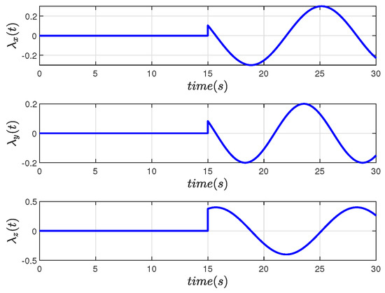
Figure 2.
Actuator Anomalies for Position Channel.
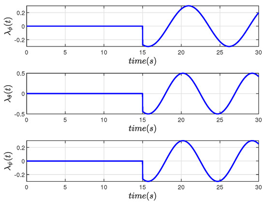
Figure 3.
Actuator Anomalies for Attitude Channel.
The simulation results of the proposed FTC scheme are shown in Figure 4, Figure 5, Figure 6 and Figure 7.
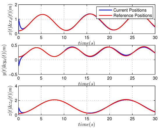
Figure 4.
UAV’s Position Tracking Performance.
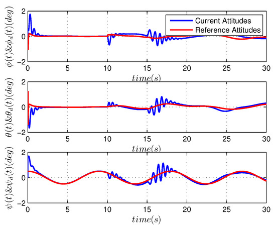
Figure 5.
UAV’s Attitude Tracking Performance.
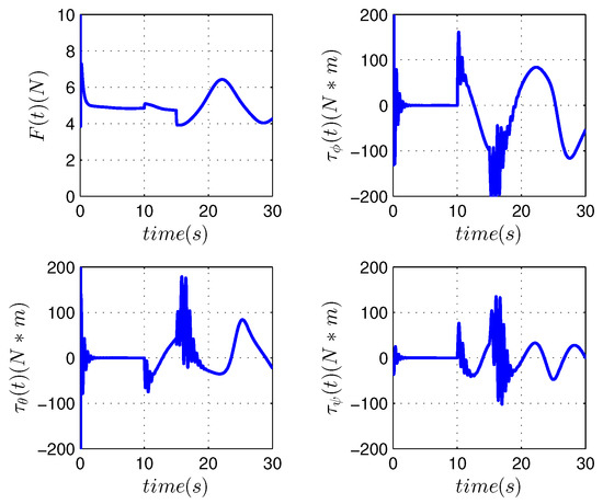
Figure 6.
UAV’s Control Inputs.
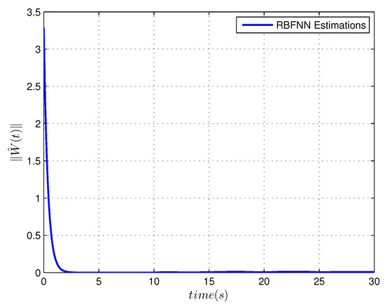
Figure 7.
RBFNN Weights of Position Control.
Figure 4 and Figure 5 show the UAV’s position and attitude tracking control performances. In Figure 4, it is shown that the current position can well follow the predefined trajectory even should actuator anomalies happen. In Figure 5, the current attitude can follow the desired attitude from the initial state quickly, and the tracking errors suddenly changes within when the actuator anomalies happen, which recovers to perfect tracking performance in about 4s. The robustness of the proposed FTC scheme can be tested and verified through inserting external disturbances of different amplitudes, which ensures the range of the variation and the response time within some reasonable values.
The control inputs, including the total thrust and torques, are illustrated in Figure 6. When the actuator anomalies happen, the thrust and torques produced by each motor change violently and then restore to their normal values. From Figure 7, the boundedness of RBFNN weights can be seen, which are coincident with (22).
5.2. Comparison and Analysis of the Results
For comparison purposes, an SM-based FTC scheme was implemented under identical circumstances. The simulation results are shown in Figure 8 and Figure 9.
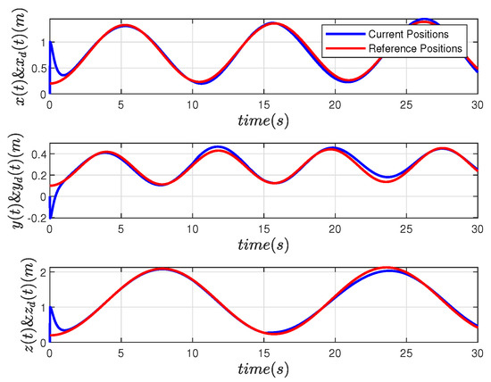
Figure 8.
UAV’s Position Tracking Performance: SM.
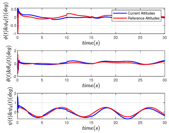
Figure 9.
UAV’s Attitude Tracking Performance: SM.
In order to quantitatively show the differences between the two controllers, the MAX offset and the root-mean-square (RMS) errors after the actuator anomalies happened were introduced and are listed in Table 1.

Table 1.
Analysis of Control Errors.
From Table 1, it can be seen that most MAX offsets and RMS errors of the proposed control scheme are smaller than that of the SM controller. Thus, the effectiveness and better performance of the proposed FTC strategy are verified.
6. Conclusions
With the development of the tri-rotor UAV, actuator anomalies have became increasingly frequent. To solve this problem, the authors of the present study aimed to propose a robust trajectory tracking control method to realize the robust tracking control of the tri-rotor UAV under abnormal actuator behavior together with external disturbances, as few existing works have taken this into consideration. The actuator anomalies were modeled as time-varying multiplicative parameters to further improve modeling accuracy. RBFNN was utilized to compensate for the actuator anomalies and external disturbances, and then the feedback linearization method was employed for the outer-loop position tracking control. The RISE-based controller was then designed to realize the inner-loop attitude tracking control with actuator anomalies and external disturbances. A Lyapunov-based analysis was used to prove the composite stability of the cascaded system. Numerical simulations and a comparison with the SM control method validated the superior performance and robustness of the proposed control strategy. Future work will focus on other kinds of neural networks to estimate the unknown actuator anomalies and external disturbances and other nonlinear FTC designs. Furthermore, building the UAV testbed and real-time experimental verifications are also under consideration.
Author Contributions
Conceptualization, W.M. and W.H.; methodology, W.H. and H.W.; software, P.W.; validation, M.H., W.M. and W.H.; formal analysis, M.H.; investigation, P.W.; resources, H.W.; data curation, H.W. and W.H.; writing—original draft preparation, W.M.; writing—review and editing, W.H.; visualization, H.W.; supervision, M.H.; project administration, W.M.; funding acquisition, W.H. All authors have read and agreed to the published version of the manuscript.
Funding
This research was funded by the National Natural Science Foundation of China under grant number 62103060, the Natural Science Foundation of Shandong Province under Grant numbers ZR2019PF021 and ZR2020MF142 and China University Innovation Fund under grant number 2021ZYA07001.
Institutional Review Board Statement
Not applicable.
Informed Consent Statement
Not applicable.
Data Availability Statement
Not applicable.
Conflicts of Interest
The authors declare no conflict of interest.
References
- Chen, F.; Jiang, R.; Zhang, K.; Jiang, B.; Tao, G. Robust backstepping sliding mode control and observer-based fault estimation for a quadrotor UAV. IEEE Trans. Ind. Electron. 2016, 63, 5044–5056. [Google Scholar] [CrossRef]
- Liu, H.; Xi, J.; Zhong, Y. Robust attitude stabilization for nonlinear quadrotor systems with uncertainties and delays. IEEE Trans. Ind. Electron. 2017, 64, 5585–5594. [Google Scholar] [CrossRef]
- Yoo, D.; Oh, H.; Won, D.; Tahk, M. Dynamic modeling and stabilization techniques for tri-rotor unmanned aerial vehicles. Int. J. Aeronaut. Space Sci. 2010, 11, 167–174. [Google Scholar] [CrossRef]
- Gu, X.; Xian, B.; Li, J. Model free adaptive control design for a tilt trirotor unmanned aerial vehicle with quaternion feedback: Theory and implementation. Int. J. Adapt. Control 2022, 36, 122–137. [Google Scholar] [CrossRef]
- Hao, W.; Ma, W.; Yuan, W.; Wang, H.; Du, Y. Modeling and nonlinear robust tracking control of a three-rotor UAV based on RISE method. IEEE Access 2021, 9, 38802–38809. [Google Scholar] [CrossRef]
- Liu, Z.; He, Y.; Yang, L.; Han, J. Control techniques of tilt rotor unmanned aerial vehicle systems: A review. Chin. J. Aeronaut. 2017, 30, 135–148. [Google Scholar] [CrossRef]
- Yu, L.; He, G.; Zhao, S.; Wang, X. Dynamic inversion-based sliding mode control of a tilt tri-rotor UAV. In Proceedings of the Asian Control Conference (ASCC), Kitakyushu, Japan, 9–12 June 2019; p. 18849170. [Google Scholar]
- Sun, N.; Yang, T.; Fang, Y.; Wu, Y.; Chen, H. Transportation control of double-pendulum cranes with a nonlinear quasi-PID scheme: Design and experiments. IEEE Trans. Syst. Man Cybern. Syst. 2019, 49, 1408–1418. [Google Scholar] [CrossRef]
- Xian, B.; Yang, S. Robust tracking control of a quadrotor unmanned aerial vehicle-suspended payload system. IEEE/ASME Trans. Mech. 2021, 26, 2653–2663. [Google Scholar] [CrossRef]
- Salazar-Cruz, S.; Kendoul, F.; Lozano, R.; Fantoni, I. Real-time stabilization of a small three-rotor aircraft. IEEE Trans. Aerosp. Electron. Syst. 2008, 44, 783–794. [Google Scholar] [CrossRef]
- Papachristos, C.; Alexis, K.; Tzes, A. Linear quadratic optimal position control for an unmanned tri-TiltRotor. In Proceedings of the International Conference Control, Decision and Information Technologies (CoDIT), Hammamet, Tunisia, 6–8 May 2013; pp. 708–713. [Google Scholar]
- Ali, Z.; Wang, D.; Masroor, S.; Loya, M. Attitude and altitude control of trirotor UAV by using adaptive hybrid controller. J. Control Sci. Eng. 2016, 2016, 6459891. [Google Scholar] [CrossRef]
- Yu, B.; Zhang, Y.; Qu, Y. Fault tolerant control using PID structured optimal technique against actuator faults in a quadrotor UAV. In Proceedings of the International Conference on Unmanned Aircraft Systems (ICUAS), Orlando, FL, USA, 27–30 May 2014; pp. 167–174. [Google Scholar]
- He, A.; Zhang, Y.; Zhao, H.; Wang, B.; Gao, Z. Adaptive fault-tolerant control of a hybrid VTOL UAV against actuator faults and model uncertainties under fixed-wing mode. Int. J. Aerospace Eng. 2022, 10, 8191154. [Google Scholar] [CrossRef]
- Zou, Y. Nonlinear robust adaptive hierarchical sliding mode control approach for quadrotors. Int. J. Robust Nonlin. 2016, 27, 925–941. [Google Scholar] [CrossRef]
- Guo, J.; Qi, J.; Wu, C. Robust fault diagnosis and fault-tolerant control for nonlinear quadrotor unmanned aerial vehicle system with unknown actuator faults. Int. J. Adv. Robot. Syst. 2021, 2, 1–14. [Google Scholar] [CrossRef]
- Zhang, Y.; Chamseddine, A.; Rabbath, C. Development of advanced FDD and FTC techniques with application to an unmanned quadrotor helicopter testbed. J. Frank. Inst. 2013, 350, 2396–2422. [Google Scholar] [CrossRef]
- Yu, Z.; Zhang, Y.; Jiang, B.; Fu, J.; Jin, Y. A review on fault-tolerant cooperative control of multiple unmanned aerial vehicles. Chin. J. Aeronaut. 2021, 35, 1–18. [Google Scholar] [CrossRef]
- Zhao, W.; Liu, H.; Lewis, F. Data-driven fault-tolerant control for attitude synchronization of nonlinear quadrotors. IEEE Trans. Autom. Control. 2021, 66, 5584–5591. [Google Scholar] [CrossRef]
- Nguyen, T.; Saussie, D.; Saydy, L. Design and experimental validation of robust self-scheduled fault-tolerant control laws for a multicopter UAV. IEEE/ASME Trans. Mech. 2021, 26, 2548–2557. [Google Scholar] [CrossRef]
- Zou, Y.; Xia, R. Robust fault-tolerant control for underactuated takeoff and landing UAVs. IEEE Trans. Aero. Elec. Sys. 2020, 56, 3545–3555. [Google Scholar] [CrossRef]
- Shen, Q.; Jiang, B.; Shi, P. Active fault-tolerant control against actuator fault and performance analysis of the effect of time delay due to fault diagnosis. Int. J. Contr. Autom. 2017, 15, 537–546. [Google Scholar] [CrossRef]
- Falcon, G.; Holzapfel, F. Adaptive fault tolerant control allocation for a hexacopter system. In Proceedings of the 2016 American Control Conference (ACC), Boston, MA, USA, 6–8 July 2016; pp. 6760–6766. [Google Scholar]
- Xian, B.; Hao, W. Nonlinear robust fault-tolerant control of the tilt trirotor UAV under rear servo’s stuck fault: Theory and experiments. IEEE Trans. Ind. Informat. 2019, 15, 2158–2166. [Google Scholar] [CrossRef]
- Hao, W.; Xian, B.; Xie, T. Fault tolerant position tracking control design for a tilt tri-rotor unmanned aerial vehicle. IEEE Trans. Ind. Electron. 2022, 69, 604–612. [Google Scholar] [CrossRef]
- Xian, B.; Diao, C.; Zhao, B.; Zhang, Y. Nonlinear robust output feedback tracking control of a quadrotor UAV using quaternion representation. Nonlinear Dynam. 2015, 79, 2735–2752. [Google Scholar] [CrossRef]
- Wen, G.; Hao, W.; Feng, W.; Gao, K. Optimized backstepping tracking control using reinforcement learning for quadrotor unmanned aerial vehicle system. IEEE Trans. Syst. Man Cy.-S. 2022, 52, 5004–5015. [Google Scholar] [CrossRef]
- Cai, Z.; de Queiroz, M.; Dawson, D. A sufficiently smooth projection operator. IEEE Trans. Autom. Control 2006, 51, 135–139. [Google Scholar] [CrossRef]
- Kendoul, F.; Yu, Z.; Nonami, K. Guidance and nonlinear control system for autonomous flight of minirotorcraft unmanned aerial vehicles. J. Field Robot. 2010, 27, 311–334. [Google Scholar] [CrossRef]
- Sontag, E. Smooth stabilization implies coprime factorization. IEEE Trans. Autom. Control 1988, 34, 435–443. [Google Scholar] [CrossRef]
- Zhao, B.; Xian, B.; Zhang, Y.; Zhang, X. Nonlinear robust adaptive tracking control of a quadrotor UAV via immersion and invariance methodology. IEEE Trans. Ind. Electron. 2015, 62, 2891–2902. [Google Scholar] [CrossRef]
- Xian, B.; Dawson, D.; de Queiroz, M.; Chen, J. Continuous asymptotic tracking control strategy for uncertain multi-input nonlinear systems. IEEE Trans. Autom. Control 2004, 49, 1206–1211. [Google Scholar] [CrossRef]
- Sepulchre, R.; Jankovic, M.; Kokotovic, P. Constructive Nonlinear Control; Springer: New York, NY, USA, 1997. [Google Scholar]
- Kendoul, F. Nonlinear hierarchical flight controller for unmanned rotorcraft: Design, stability, experiments. J. Guid. Control Dynam. 2009, 32, 1954–1958. [Google Scholar] [CrossRef]
Disclaimer/Publisher’s Note: The statements, opinions and data contained in all publications are solely those of the individual author(s) and contributor(s) and not of MDPI and/or the editor(s). MDPI and/or the editor(s) disclaim responsibility for any injury to people or property resulting from any ideas, methods, instructions or products referred to in the content. |
© 2023 by the authors. Licensee MDPI, Basel, Switzerland. This article is an open access article distributed under the terms and conditions of the Creative Commons Attribution (CC BY) license (https://creativecommons.org/licenses/by/4.0/).