Article

Reinforcement Learning-Based Control of Single-Track Two-Wheeled Robots in Narrow Terrain

1
Department of Automation, Tsinghua University, Beijing 100084, China
2
School of Mechatronics Engineering, Harbin Institute of Technology, Harbin 150006, China
*
Author to whom correspondence should be addressed.
Actuators 2023, 12(3), 109; https://doi.org/10.3390/act12030109
Submission received: 30 January 2023 / Revised: 24 February 2023 / Accepted: 25 February 2023 / Published: 28 February 2023
(This article belongs to the Special Issue Advanced Technologies and Applications in Robotics)

Abstract

:
The single-track two-wheeled (STTW) robot has the advantages of small size and flexibility, and it is suitable for traveling in narrow terrains of mountains and jungles. In this article, a reinforcement learning control method for STTW robots is proposed for driving fast in narrow terrain with limited visibility and line-of-sight occlusions. The proposed control scheme integrates path planning, trajectory tracking, and balancing control in a single framework. Based on this method, the state, action, and reward function are defined for narrow terrain passing tasks. At the same time, we design the actor network and the critic network structures and use the twin delayed deep deterministic policy gradient (TD3) to train these neural networks to construct a controller. Next, a simulation platform is formulated to test the performances of the proposed control method. The simulation results show that the obtained controller allows the STTW robot to effectively pass the training terrain, as well as the four test terrains. In addition, this article conducts a simulation comparison to prove the advantages of the integrated framework over traditional methods and the effectiveness of the reward function.

1. Introduction

A single-track two-wheeled (STTW) robot is an autonomous mobile robot with the structure of an unmanned bicycle or motorcycle. It is called an STTW robot due to the overlap of the driving trajectories of the front and rear wheels. It is characterized by a speed block, small size, simple structure, and strong off-road capability, with potential future applications. The STTW robot is an underactuated system, with static instability and dynamic stability. Therefore, over the years, some researchers have studied the balance control of STTW robots at normal driving speeds [1,2,3]. As the related research has progressed, scholars have explored the balance control of STTW robots in a high-speed state [4], low-speed state [5], zero-speed state [6,7,8], and in the situation of avoiding obstacles [9]. However, these previous works are not thorough regarding the problem of STTW robots driving in unstructured terrain.
Passing through narrow terrain is an advantage of STTW robots, and studying this task can exert the high adaptability of such robots. Narrow terrain is more common in mountainous and jungle terrain, which includes stones and trees, produces fog during the day, and lacks lights at night. These complex situations create low visibility and line-of-sight occlusions. In low visibility conditions, STTW robots can only detect limited geographical information, which cannot support global path planning, and line-of-sight occlusions mean that the robot cannot obtain comprehensive geographic information, so it needs to be more cautious and robust in making decisions. Therefore, this article studies the control of STTW robots in narrow terrain with limited visibility and line-of-sight occlusions. In narrow terrain passing tasks, the path planning, tracking control, and balancing control of STTW robots are highly coupled, which makes the control task more complicated. For instance, the path planned by STTW robot tracking needs to meet the kinematic and dynamic characteristics, and the balance of the robots needs to be considered in the process of trajectory tracking. Therefore, the STTW robot control method proposed in this paper integrates the local path planning, the trajectory tracking, and the balance control in a single framework, which enables this challenging coupled problem to be solved.
Compared to traditional path planning and control methods, using deep reinforcement learning to achieve narrow terrain passing tasks has certain advantages. First, the deep reinforcement learning can integrate path planning and control under a single framework. In this way, planning and control algorithms do not need to be designed separately. Second, this article uses a model-free reinforcement learning algorithm to solve the problem, which avoids building a dynamic model for the STTW robot. In addition, the reinforcement learning is more advantageous in the handling control problem with a sophisticated state space. Our solution for the STTW robot’s narrow terrain passing task can be summarized as shown in Figure 1.
The primary contributions of this article are as follows:
  • This article proposes a deep reinforcement learning-based STTW robot control method, which integrates local path planning, trajectory tracking, and balance control in a single framework.
  • The proposed control method is applied to realize STTW robot driving in narrow terrain with line-of-sight occlusions and limited visibility. To the best of our knowledge, this paper is the first to study STTW robots in such an environment.
  • The proposed method offers good generalization to terrain other than that used during training.
The rest of this paper is organized as follows. In Section 2, some related research activities are offered. Section 3 presents the design of the control method for STTW robots. Simulation settings are provided in Section 4. In Section 5, the training results and some comparative simulations are given. The final section provides the conclusion of this article.

2. Related Work

2.1. Reinforcement Learning

Reinforcement learning (RL) is a type of machine learning that learns the Markov decision process (MDP) of the optimal strategy by allowing the agent to continuously interact with the environment through a “trial and error” approach. Mnih et al. [10] used deep learning [11] combined with Q-learning [12] and proposed a deep Q-network (DQN). The DQN uses the experience replay mechanism [13] and target network technology to solve the problem of unstable training. However, Q-learning has the problem of overestimating the action-value function. Hasselt et al. [14] proposed a double DQN (DDQN) algorithm based on the DQN and double Q-learning algorithm to solve this problem. Combining the ideas of the deterministic policy gradient [15], the actor-critic (AC) [16,17,18] algorithm, and DQN, Lillicrap et al. proposed the deep deterministic policy gradient (DDPG) [19] to realize the robot control task in continuous action space. Many scholars have improved the DDPG [20,21,22], of which the most influential is the twin delayed deep deterministic policy gradient (TD3) [23]. To ensure that policy optimization is performed in a non-deteriorating direction, Schulman et al. proposed trust region policy optimization (TRPO) [24]. To address the fact that the optimization problem in TRPO is challenging to solve and has high computational complexity, the proximity policy optimization (PPO) method [25] uses pruning technology to approximate the TRPO’s objective function. Furthermore, Haarnoja et al. combined the AC and maximum entropy model to propose the soft actor-critic method (SAC) [26]. In recent years, many studies have also applied reinforcement learning to STTW robots [27,28], but these works do not involve the path planning and trajectory tracking of STTW robots.

2.2. STTW Robots

The STTW robots have a variety of solutions for maintaining balance. Sun et al. [3] proposed a fuzzy state space model of STTW robots with different velocities and designed a fuzzy controller optimized by an improved particle swarm optimization algorithm with two stages. Suryanarayanan et al. [4] present automated roll-rate control for high-speed STTW robots. Guo et al. [29] modeled the robot dynamics based on feature selection and RHONN and designed a controller to realize the balance control of uneven terrain. Furthermore, many scholars have added additional actuators to solve the underactuated problem of the robot system. The authors of [30] and [31] used the gyro effect of the control moment gyroscope (CMG) to keep the robot balanced. Seekhaoa et al. [32] achieved the balance control of the robot by applying a pendulum mass through a linear–quadratic regulator. Hwang et al. [33] added a pendulum balance to the robot and designed a fuzzy sliding-mode underactuated controller to maintain balance by improving the sliding-mode control [34]. In addition, the authors of [35] and [36] used reaction wheels to keep the robot balanced. However, none of these studies involved path planning.
The problem of obstacle avoidance and path planning for mobile robots has been extensively studied over the decades. The artificial potential field (APF) [37] guides the robot to the goal position by building a potential virtual field, and this method can adapt to low visibility environments. However, the APF has a significant weakness in that APF may be trapped in local optima or oscillate in narrow spaces. Rapidly exploring random trees star (RRT*) and probabilistic roadmap (PRM) are sample-based algorithms [38] that are probabilistically complete and highly efficient, especially if the constraints are complex. According to the unique characteristics of STTW robots, Zhao et al. [39] proposed a detection model to detect obstacles, including those with line-of-sight occlusion conditions, and a local path planning method to avoid detected obstacles by using four phases to re-plan the path. Although the above approaches for path planning involve line-of-sight occlusions or limited visibility, these studies do not use reinforcement learning.
In order to solve the trajectory tracking problem of STTW robots, Keo et al. [7] carried out the trajectory tracking control of STTW robots using the input-output linearization approach. This work is the first systematic study of the joint control of balance and trajectory tracking for an STTW robot with a pendulum. The authors of [40] presented a trajectory tracking and balance controller built on the attractive external-internal convertible property of the STTW robot dynamics. In [41], an STTW robot without additional actuators achieved trajectory tracking and control through model predictive control and proportion integral differential (PID). For the uncertainty of the road environment in trajectory tracking, He et al. [42] used the Gaussian process and disturbance cancellation to limit the tracking error to a small range, given by design.
This paper aims to design a control method that integrates path planning, trajectory tracking, and balance control, realizing the robot’s task in narrow terrain with low visibility and line-of-sight occlusions. The relationship between the contents of the references and the proposition of this paper is shown in Table 1. As can be seen from Table 1, the emphasis of the literature mentioned above is different, and there is no direct solution for narrow terrain passing tasks.

3. STTW Robots Control Method for Narrow Terrain

The STTW robot control method proposed in this article is developed for narrow terrain, with limited visibility and line-of-sight occlusions. STTW robot path planning needs terrain information for the terrain ahead, trajectory tracking needs the planned path and attitude information, and balance control also needs attitude information. The deep neural network can be used as the controller of the robot to process complex terrain information and attitude information, and then output the signals required by the robot’s actuator. In this way, local path planning, trajectory tracking, and balance control are integrated under a single framework. At the same time, reinforcement learning can train and optimize the neural network controller. Therefore, this article employs deep reinforcement learning as a control method to achieve the narrow terrain passing task. In this section, we define the state, action, and reward function. Second, the neural network structure inside the agent is designed. Finally, we design an algorithm to train the agent. Then, this agent can be used as the controller for the STTW robot and realize the task of passing through narrow terrain.

3.1. State

We define the state of the robot as s:
s = [ s A , s B ]
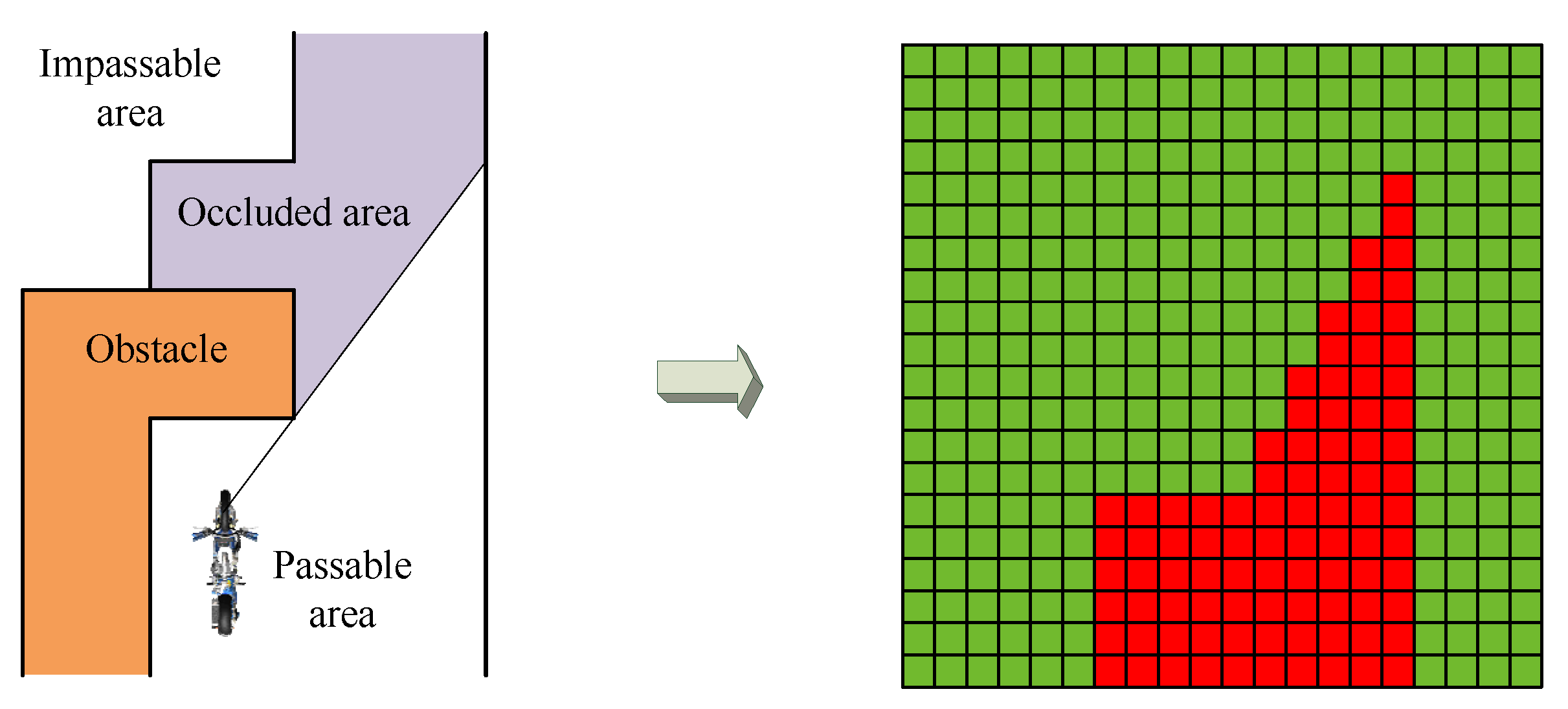
The first component, sA, is the information regarding the terrain ahead within D1 meters. The geographic information of the front can be obtained by lidar and by camera, then transformed into passable and non-passable areas by the perception system. The terrain information needs to be discretized. First, the geographic information located D1 meters in front of the STTW robot and D2 meters on the left and right are sampled. One point is sampled every D1/40 meter in the front, and one point is sampled every D2/20 meter in the lateral direction. The sampling point records the condition of passability at the location. The passable area is marked as 1, and the impassable area is marked as −1. Finally, these data can form a 41 × 41 matrix. This process is shown in Figure 2. (The primary purpose of Figure 2 is to illustrate the process, and the number of sampling points is not consistent with the number used in the method.)
The second component, sB, is a ten-dimensional vector representing the robot’s attitude and action information as follow:
s B   = [ a k 1 , v p , θ , θ ˙ , ψ Y , ψ R , ψ ˙ Y , ψ ˙ R , ψ ¨ Y , ψ ¨ R ]
where  a k 1  represents the action at the previous moment, and  v p  indicates the speed of the robot.  θ  and  θ ˙  represent the angle and angular velocity of the robot’s front wheel steering.  ψ Y ψ ˙ Y , and  ψ ¨ Y  represent the robot’s yaw angle, yaw angular velocity, and yaw angular acceleration, and  ψ R ψ ˙ R , and  ψ ¨ R  represent the robot’s roll angle, roll angular velocity, and roll angular acceleration. The system coordinates for the STTW robot are shown in Figure 3.

3.2. Action

In this paper, the task of passing through narrow terrain is assumed to be a fixed-speed driving task. The robot needs to maintain balance and steer through the steering, so the action a taken by the agent is the steering torque.  a = [ F s t ] F s t  represent the rotational torque needed by the robot’s steering motor.

3.3. Reward Shaping

To successfully pass through narrow terrain, we construct an efficient reward function:  r = C 1 C 2 , where C1 represents the reward obtained by the STTW robot during the driving process. (The longer the distance traveled, the higher the reward obtained.) C2 represents the penalty assigned when the robot falls into a canyon or hits an obstacle. The mathematical description of C1 and C2 depends on the training terrain parameters, which will be given in Section 4. This paper aims to allow the robot to pass through narrow terrain safely, so we do not seek the shortest path or smaller steering torque when designing the reward function.

3.4. Network Structure

The control method adopted in this article has two critic networks with the same structure and one actor network. The structures of the networks are shown in Figure 4. Figure 4a depicts the actor network, with two inputs: terrain information sA and robot attitude information sB. Since the terrain information is a 41 × 41 matrix, it is processed by the convolutional neural network and then plugged into fully connected layer 1. The networks designed in this paper use the cross-channel normalization layer to enhance the generalization ability of the controller. The layer uses each input element e to compute the normalized element e′, as follow:
e = e ( K c + α c · s c W c ) η
where Kc, αc, and η are the hyperparameters, and sc represents the sum of squares of the elements in the normalization. Wc is the window channel size.
The attitude information sB is directly plugged into fully connected layer 2, and then, together with the output vector from fully connected layer 1, the information is input into fully connected layer 3 through the ReLU layer. After several layers, the 2-dimensional actions are obtained. Compared with the actor network, the critic network must add an action input. The critic network’s output is also a one-dimensional action value that is used to evaluate the quality of the actor network’s output action value.

3.5. Training Algorithm

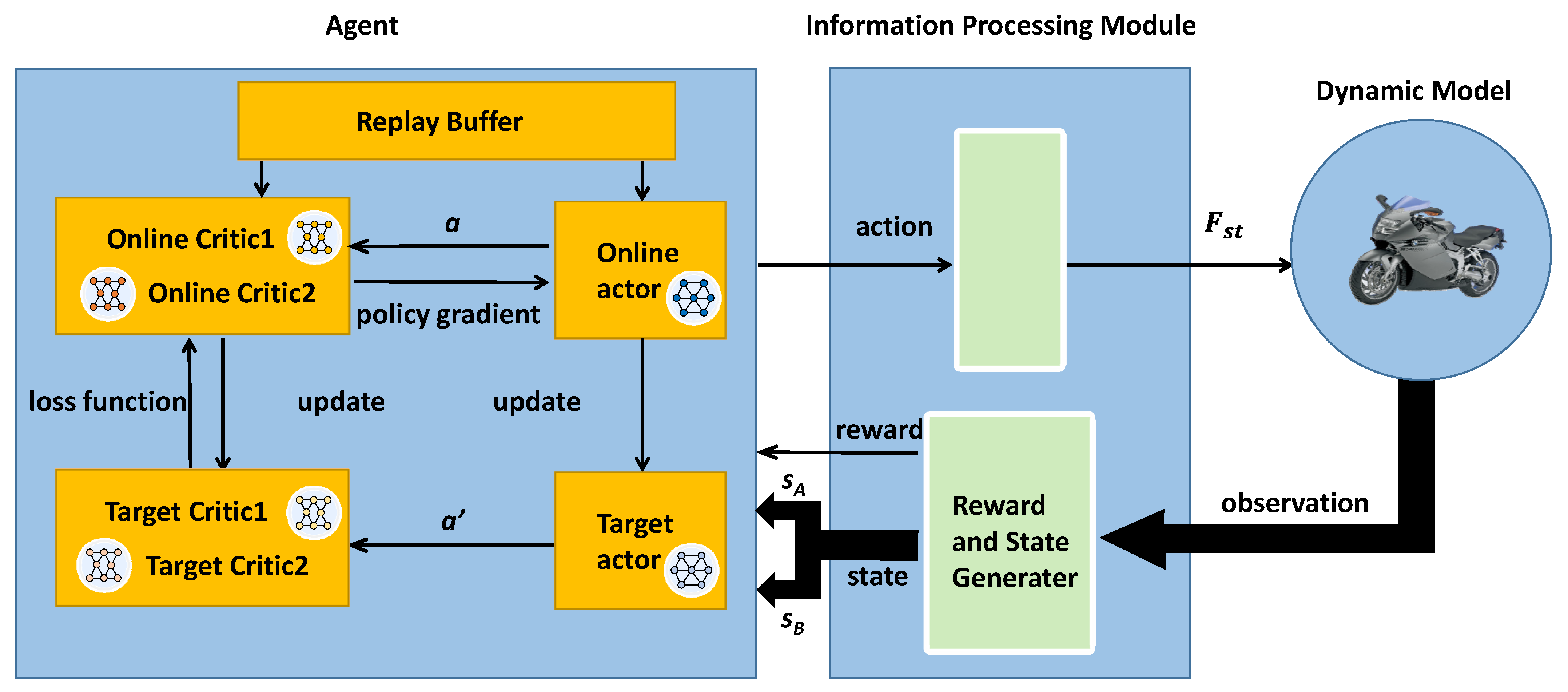
This article uses a reinforcement learning algorithm, TD3, as the training algorithm. The overall training framework is shown in Figure 5. The agent has six neural networks: critic network 1  Q 1 ( s , a ) , critic network 2  Q 2 ( s , a ) , actor network  μ ( s ) , target critic network 1  Q 1 ( s , a ) , target critic network 2  Q 2 ( s , a ) , and target actor network  μ ( s ) . During the training process, the actor network generates an action input for the information processing module. Then, the information processing module converts the action into the STTW robot’s steering torque and plugs it into the dynamic model. The dynamic model is solved according to the input, and then the solved robot position and attitude data are transmitted to the information processing module. The information processing module calculates the states sA, sB, and the reward value r, according to these data, and transmits them to the agent. The agent uses the data in the replay buffer to update the network. The training algorithm is described as follows:
Firstly, the replay buffer β is initialized. The critic network parameters  θ Q k  and actor network parameters  θ μ  are randomly initialized, and the target critic network and actor network are then initialized with the same parameter:  θ Q k = θ Q k  and  θ μ = θ μ , where k = 1 is the first critic network, and k = 2 is the second critic network.
For each training time step:
  • According to the current observation s, select action  a = μ ( s ) + N ,  where N is stochastic noise, using Gaussian noise with variance decay.
  • Execute action  a  to interact with the dynamic model and return the reward  r  and the next observation  s  to the agent.
  • Store the obtained data  ( s , a , r , s )  in the replay buffer β.
  • From the replay buffer, select a random mini-batch of K samples  ( s i , a i , r i , s i ) i = 1 , 2 , K .
  • The critic network  θ Q k  is updated by minimizing the loss L:
    L = 1 K i = 1 K ( y i Q k ( s i , a i | θ Q k ) ) 2
    where
    y i = { r i r i + γ min k ( Q k ( s i , c l i p ( μ ( s i | θ μ ) + ε , a min , a max ) | θ Q k ) ) If   s i   is   a   terminal   state else
    and  γ  is a discount factor that determines the priority for short-term rewards.  a min  and  a max  represent the action’s minimum and maximum values.  ε  is stochastic noise, using Gaussian noise with variance decay; and the clip function is used to clip the action based on  a min  and  a max , which keeps the target close to the original action.
  • Every 2 steps, update the actor network  θ μ  using the deterministic policy gradient to maximize the expected discounted reward J, as follows:
    θ μ J 1 K i = 1 K G a i G μ i
    where  G a i = a min k ( Q k ( s i , a | θ Q ) )
    • a = μ ( s i | θ μ )
    • and  G μ i = θ μ μ ( s i | θ μ )
  • Every 2 steps, target actor network  θ μ  and target critic network  θ Q k  are updated using a soft-updating technique with smoothing factor τ, as follows:
    θ μ τ θ μ + ( 1 τ ) θ μ
    θ Q τ θ Q + ( 1 τ ) θ Q

4. Simulation Settings

4.1. Simulation Platform

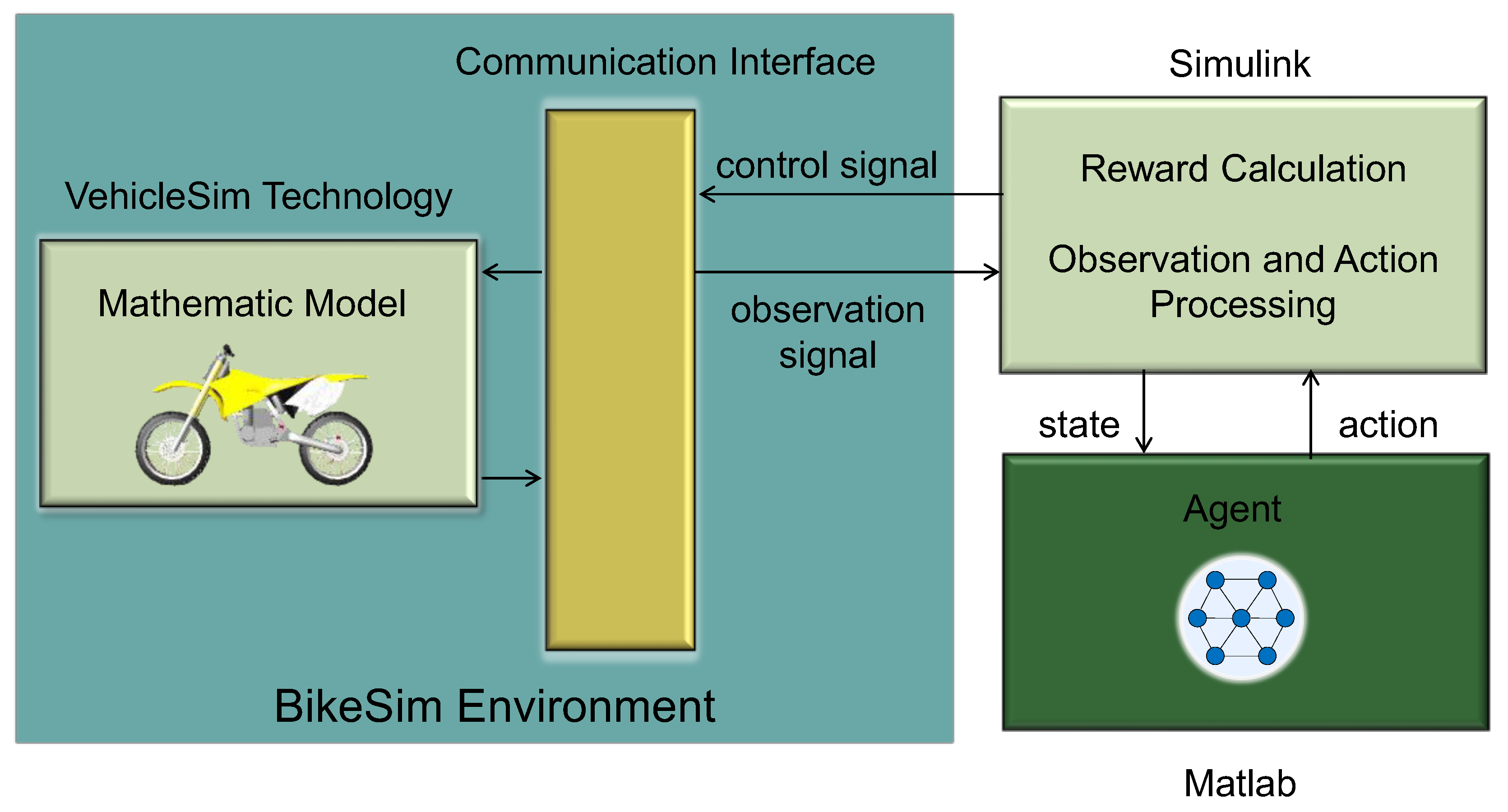
In this study, we used MATLAB/Simulink and BikeSim as the simulation platform, as shown in Figure 6. BikeSim [43] is a multi-body dynamics simulation software widely used in the dynamic researches of STTW vehicles [44,45]. BikeSim used VehicleSim (VS) technology to provide ordinary differential equations for a multibody dynamic model. Meanwhile, BikeSim and Simulink have a communication interface. Therefore, BikeSim can transmit the STTW robot’s (motorcycle’s) position and attitude information to Simulink, and Simulink processes these data and generates the state s, reward value r, and termination signal. Simulink then transmits the generated data to the agent, which is simulated in MATLAB. In addition, in MATLAB, the agent generates actions and transmits them to Simulink. Simulink converts the action into steering torque and transmits it to BikeSim. From the agent’s point of view, Simulink and BikeSim are equivalent to the reinforcement learning environment. From the STTW robot’s point of view, MATLAB/Simulink is equivalent to a controller.

4.2. Training Terrain Structure

The terrain structure map used for training is shown in Figure 7. The total length of the runway was 100 m, the width of the narrow section was 1 m, and the runway was 3 m above the ground. There was a platform of the runway 8 m long and 2 m wide at 15 and 35 m, and there was a platform of the runway 10 m long and 3 m wide at 55 m. There were two obstacles on both sides of the runway at 63 m, and the road width between the obstacles was 0.8 m.

4.3. Simulation Parameter Settings

Regarding the relevant parameters of reinforcement learning, the control frequency was 25 Hz. The maximum duration of each episode was 11 s, and the discount factor  γ  used in Equation (5) was 0.998. The noise variance of the output action and the noise variance decay rate were 0.35 and 10−6. The size of random experience mini-batch K used in Equations (4) and (6) was 250. The target network update smoothing factor τ used in Equations (7) and (8) was 10−3. The learning rate of the actor network was 10−4, and the learning rates of the critic networks were 10−3 and 1.5 × 10⁻³. To set the sampling points, D1 was set to 10 m, and D2 was set to 2.5 m. For the STTW robot’s parameter settings, the distance between the two wheels was 1.468 m, the tire width was 0.1 m, the radius of the front wheel was 0.333 m, and the rear wheel’s radius was 0.33 m. The front fork angle was 27.8 degrees, the mass was 211 kg, and the driving speed was set to 25 km/h. The robot can only perceive the terrain information 10 m ahead, meaning there were only 1.44 s during which the robot could react and adjust its attitude. Therefore, this high-speed driving task is relatively difficult. The reward function was set as follows:
r = C 1 C 2
where  C 1 = { 0 0.2 0.4 0.6 1.2 1.4 2 2.5 d 5 5 < d 10 10 < d 15 15 < d 23.5 23.5 < d 35 35 < d 43.5 43.5 < d 63.5 d 63.5  
  • and  C 2 = { 3 4 0 if   the   robot   falls   off   if   the   robot   collides   else
  • where d is the position of the robot in the X direction.

5. Results

5.1. Results after Training

After training, we constructed an STTW robot controller for narrow terrain. The trajectory of the STTW robot on the training terrain is shown in Figure 8a. When the STTW robot was 13.5 m in front of the runway, it drove in the middle of the road as much as possible and maintained its body balance. When the robot reached 13.5 m (point A), it observed that the terrain 10 m ahead may require it to turn left; therefore, it took the appropriate action of turning the front wheel to the left. As seen in Figure 8b, the front wheel began to deflect to the left at the 1.9th second. At the same time, it can be seen from Figure 8c that the body began to lean to the left. When the STTW robot had driven to 24 m (point B), the received information indicated a narrow road section with a width of one meter, so it began to adjust the angle of the front wheel. When it had driven to 31 m (point C), the robot considered that the front should turn right and adjusted the steering to deflect to the right. It can be seen from Figure 8c,d that at 4.6 s, the body leaned to the left, and the yaw angle began to gradually decrease. When the STTW robot drove to 58 m (point D), it perceived a narrower road of 0.8 m wide ahead. Therefore, it adjusted the steering angle to pass this road smoothly. Finally, the STTW robot again drove onto a narrow road with a width of 1 m and successfully completed the task of passing through all the narrow terrain.
In addition, we tested the ability of the STTW robot to achieve stable driving on straight-line terrain. The results after training are shown in Figure 9. It can be seen from the figure that the robot can maintain relatively stable straight-line driving in the case of limited sensor accuracy (0.25 m longitudinal accuracy and 0.125 m lateral accuracy).

5.2. Robustness Test

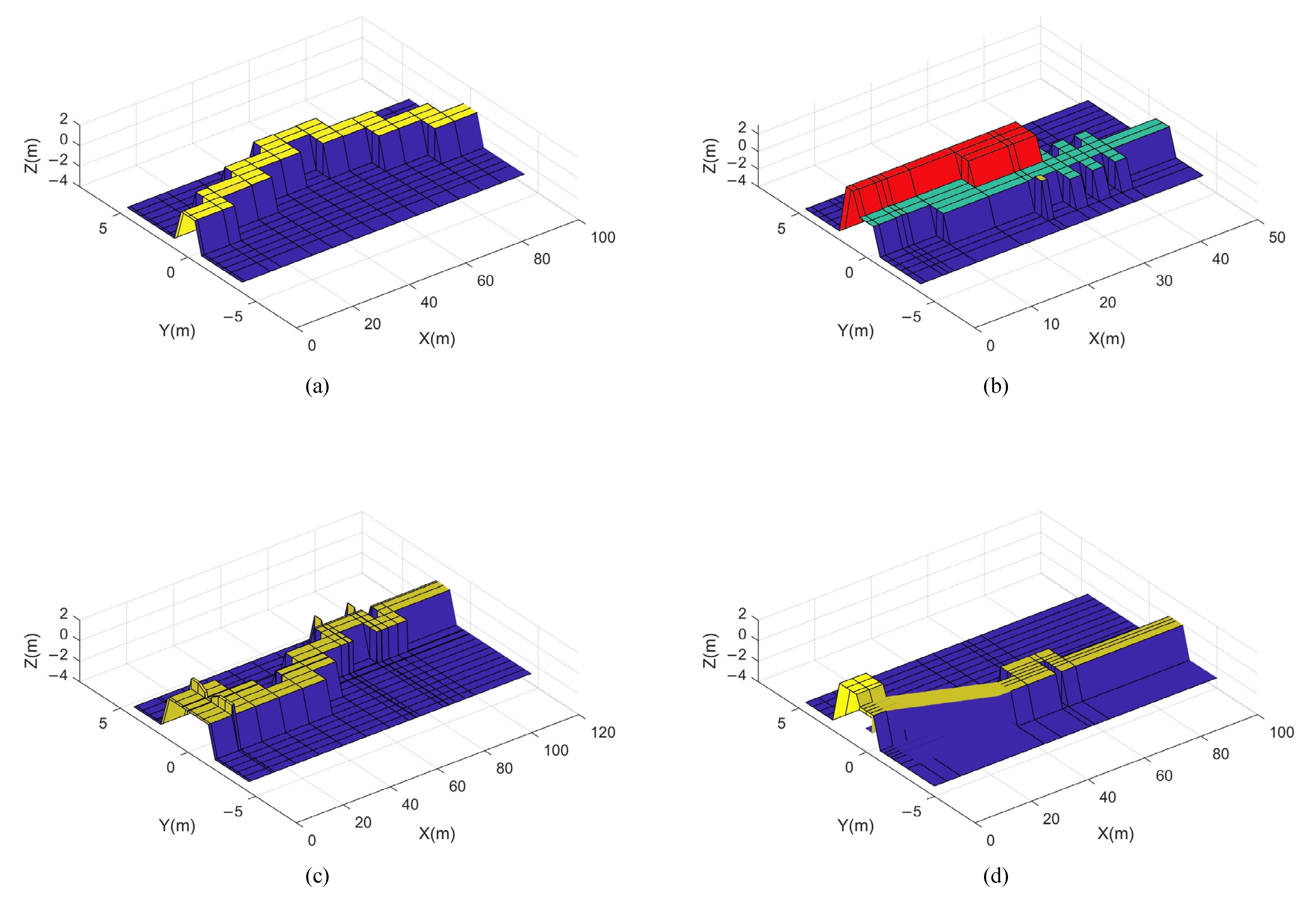
The trained controller described above was used for the STTW robot, which was tested on four additional terrains. The four test terrains are shown in Figure 10, and the execution time for each terrain is shown in Table A1. Even though the types of road conditions on the training terrains were relatively limited, the trained controllers still passed through narrower roads and more complex test terrain. On test terrain 1, there was a 5.7–11.3 degree inclination angle on the narrow terrain, and one of the platforms required that the STTW robot turn within 4 m. The STTW robot still passed over the road smoothly. On test terrain 2, an obstacle with a height of 2.5 m appeared at 18 m and blocked the robot’s sight. The obstacles that block the line-of-sight have been marked in red. When an obstacle that blocks the visibility of the robot appears, the passable areas behind obstacles are recognized as impassable areas and marked as −1 in the state sA matrix. The process is illustrated in Figure 11. At the same time, there is a raised road surface at 4 m. However, the robot was able to keep driving normally. On test terrain 3, there was considerable terrain that differed from the training terrain. In particular, there was a 0.4 m slit at 10 m, but the STTW robot successfully passed through the test terrain. On test terrain 4, we designed some narrow roads, with widths different from those in the training terrain, but they did not affect the STTW robot’s ability to pass through the terrain.
To verify the robustness of the control method proposed in this paper, we use the following three scenarios for testing:
(1)
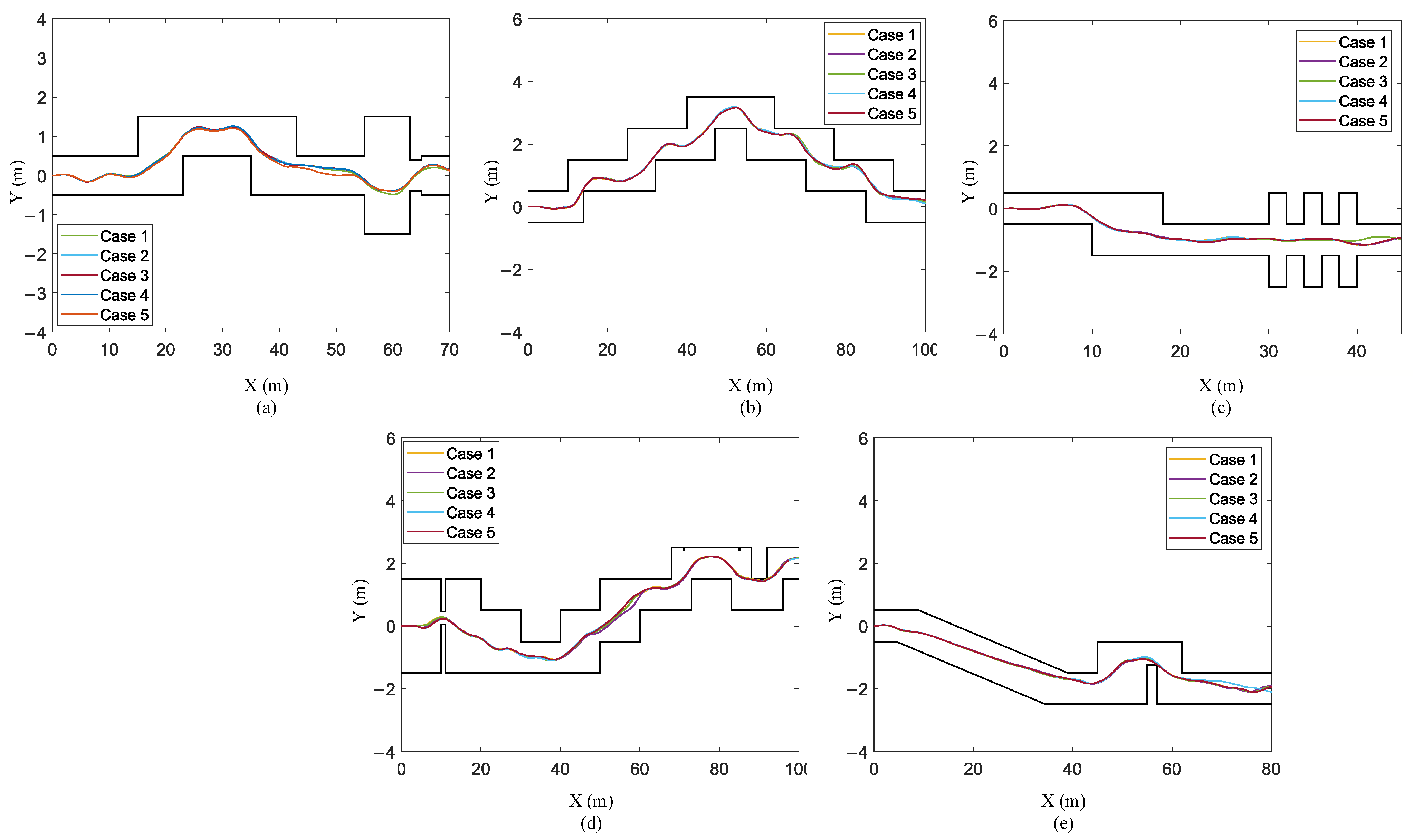
Scenario I: The actuator is disturbed. We add Gaussian noise with a mean of zero and a variance 0.01 to the action signal. The trajectories of the STTW robot on the training terrain and four test terrains are shown in Figure 12.
(2)
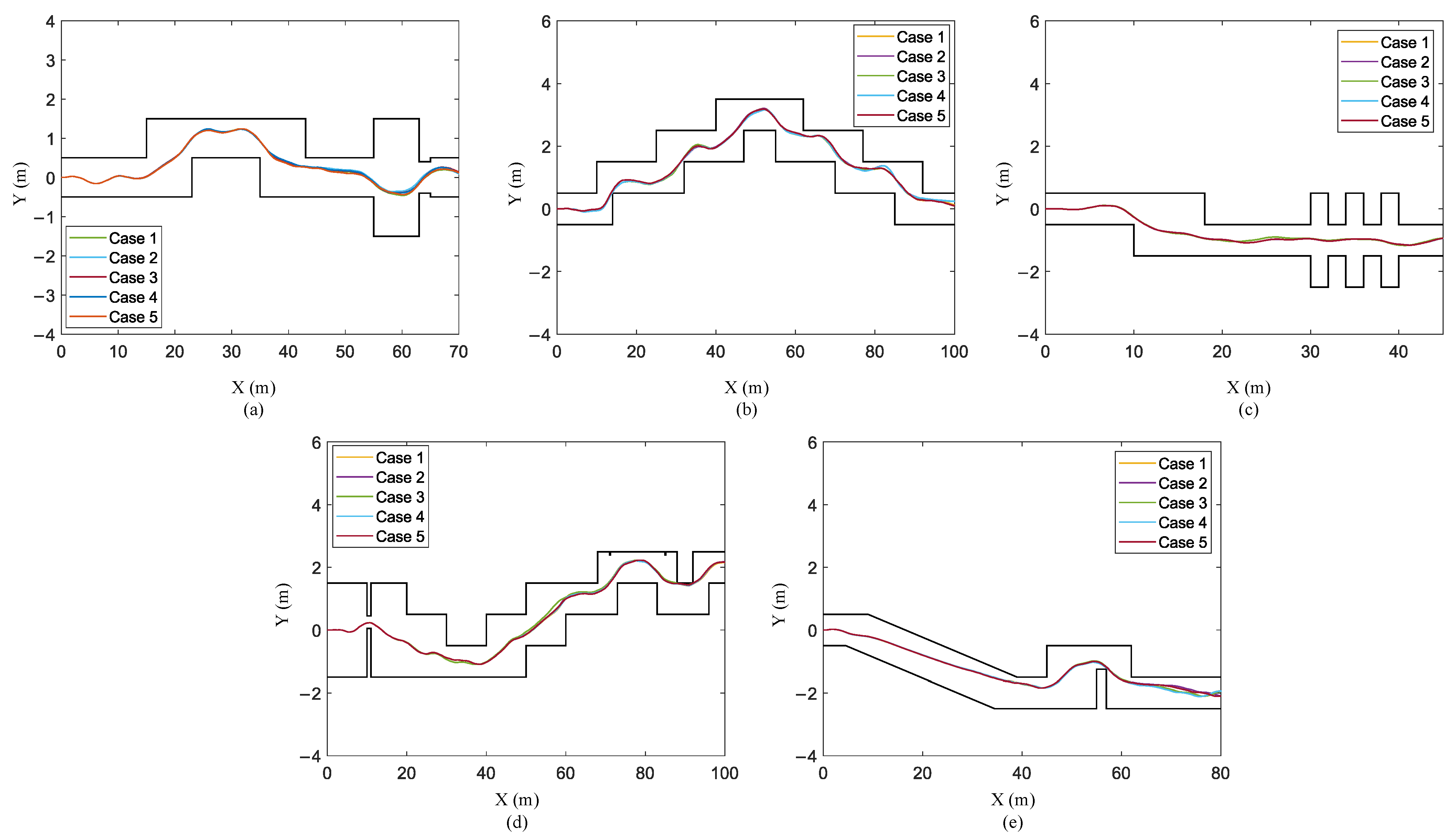
Scenario II: The main frame is disturbed by force. We added a disturbing force in the robot center, and the disturbing force obeys Gaussian noise with a mean of zero and a variance 100. We have verified it five times in training terrain and testing terrain, and the results show that the robot can overcome these disturbances and successfully pass through narrow terrain. The trajectory of the robot is shown in Figure 13.
(3)
Scenario III: The perception system has errors. Considering that the perception system is not completely reliable, we assume that there is a certain error in the obtained geographic information. In the state sA matrix, there is a 2.5% probability that the value of any row or column is set to 1 or −1. Likewise, we conducted five verifications in training terrain and testing terrain. The simulation results are shown in Figure 14. As can be seen from the figure, the robot successfully passed through these narrow terrains.

5.3. Comparison with Traditional Path Planning and Control Methods

The STTW robots pass through narrow terrain, which not only tests the ability of the control algorithm, but also the path planning ability. For the narrow terrain used in this paper, we used several traditional path planning and control methods to compare with the method in this paper. The path planning algorithms used are as follows.
  • The artificial potential field (APF) [37]. The artificial potential field method is used to design an artificial potential field  U  to guide the robot to move in an environment full of obstacles. In this method, the target point generates an attractive potential  U att  to the mobile robot, and the obstacles generate a repulsive potential  U rep  to the mobile robot. Finally, the motion of the mobile robot is controlled by seeking the resultant force as follows:
    U = U att + U rep
  • The path planning method for the intermediate step [46]. This method transforms terrain with obstacles into a simple polygon, and decomposes free space into polygons. According to the generated face graph, the method finds the sequence of polygons. Finally, this sequence is used for the planned path.
  • Variation of rapidly exploring random trees (RRT*) [38]. The original RRT algorithm uses an initial point as the root node and increases leaf nodes through random sampling. A path composed of tree nodes from the initial point to the target point can be found in the random tree. Based on the RRT algorithm, the RRT* algorithm adds a search for the adjacent nodes of the newly generated node and the process of rerouting.
In this section, the RRT* and the method in [46] were used for the global path planning of the training terrain and the four test terrains. Among them, test terrain 2 did not consider field occlusion.
Based on the planned path, we used pure pursuit as the STTW robot trajectory tracking method [47]. Lean angle  ϕ ref  is the lateral error  L t a r  multiplied by the path follower control gain  K r i d , as follows:
ϕ ref = L t a r × K r i d
The steering torque is calculated by the lean angle controller using the PID controller. The proportional gain was set to  K p = 140 0.6875 × v p , the integral gain was set to  K i = 250 + 1.875 × v p , and the derivative gain was set to  K d = 40 + 0.6 × v p v p  indicates the speed of the robot, and the unit is m/s. In order to prevent the robot from losing its balance, we set the maximum lean angle of the robot to 40 degrees and the maximum lean angle rate to 300 degrees per second.
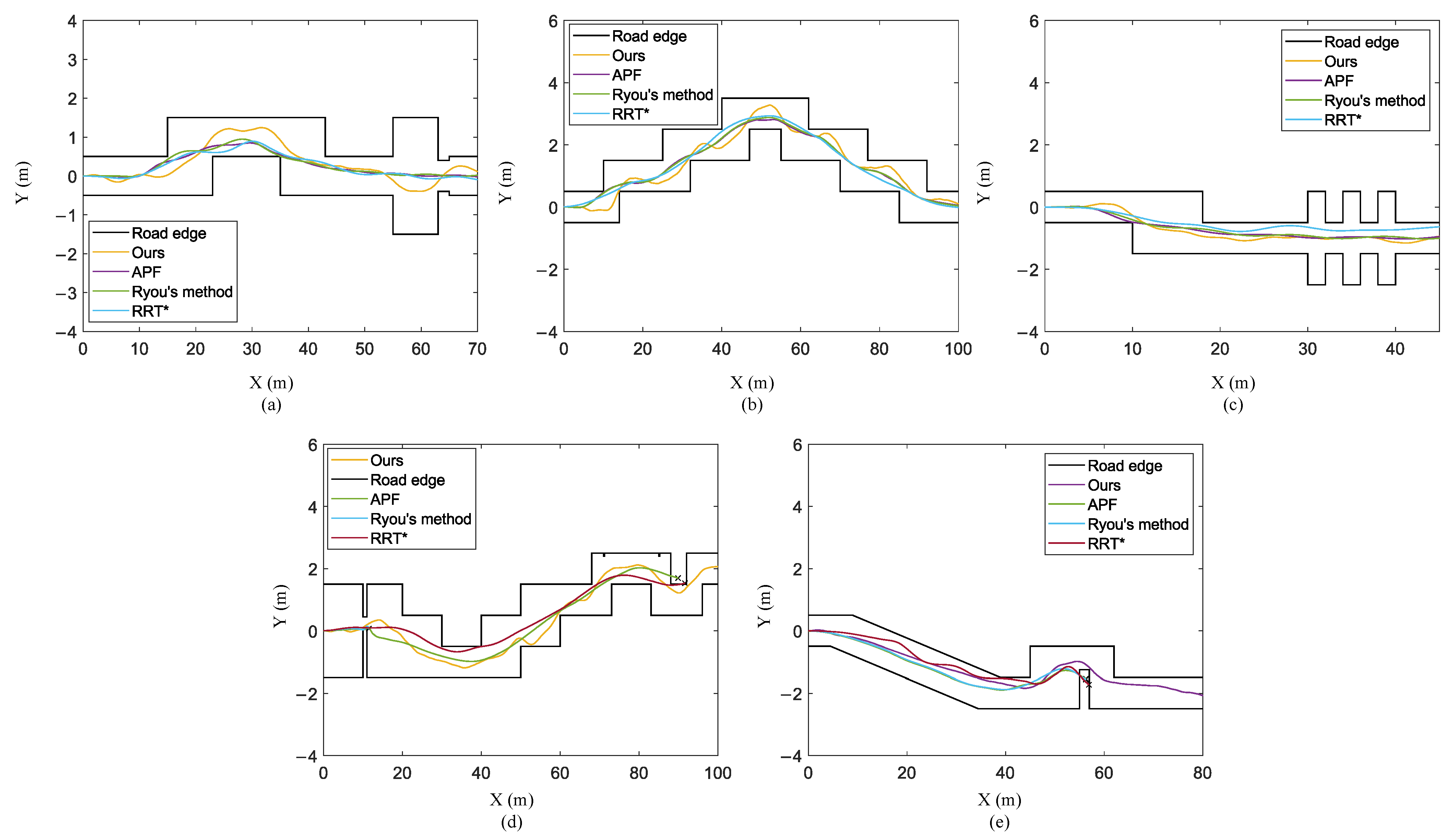
In the choice of the control gain  K r i d , we could not find a control gain that is suitable for all terrains and trajectory planning methods. Therefore, we used different control gains according to different situations. The control gain settings are shown in Table 2. However, in test terrain 3 and test terrain 4, we tried various control rates, but the STTW robot could not pass these terrains, so we used the control rate that allowed the STTW robot to travel as far as possible. The motion trajectory of the STTW robot using the above method is shown in Figure 15. In Figure 15, We denote the path planning method for the intermediate step [46] as “Ryou’s method”. Table 2 shows some terrains that cannot be passed using the traditional planning method, even considering global planning. The method proposed in this paper can only obtain terrain information 10 m in front of the robot and perform local path planning, but this method can still allow the robot to pass through some complex and narrow terrains. Although the trajectories of our method may not be perfect in some terrains, the objective of this paper is to pass the terrains. From this point of view, our method exhibits advantages in narrow terrain passing tasks.

5.4. Comparison between Different Reinforcement Learning Algorithms

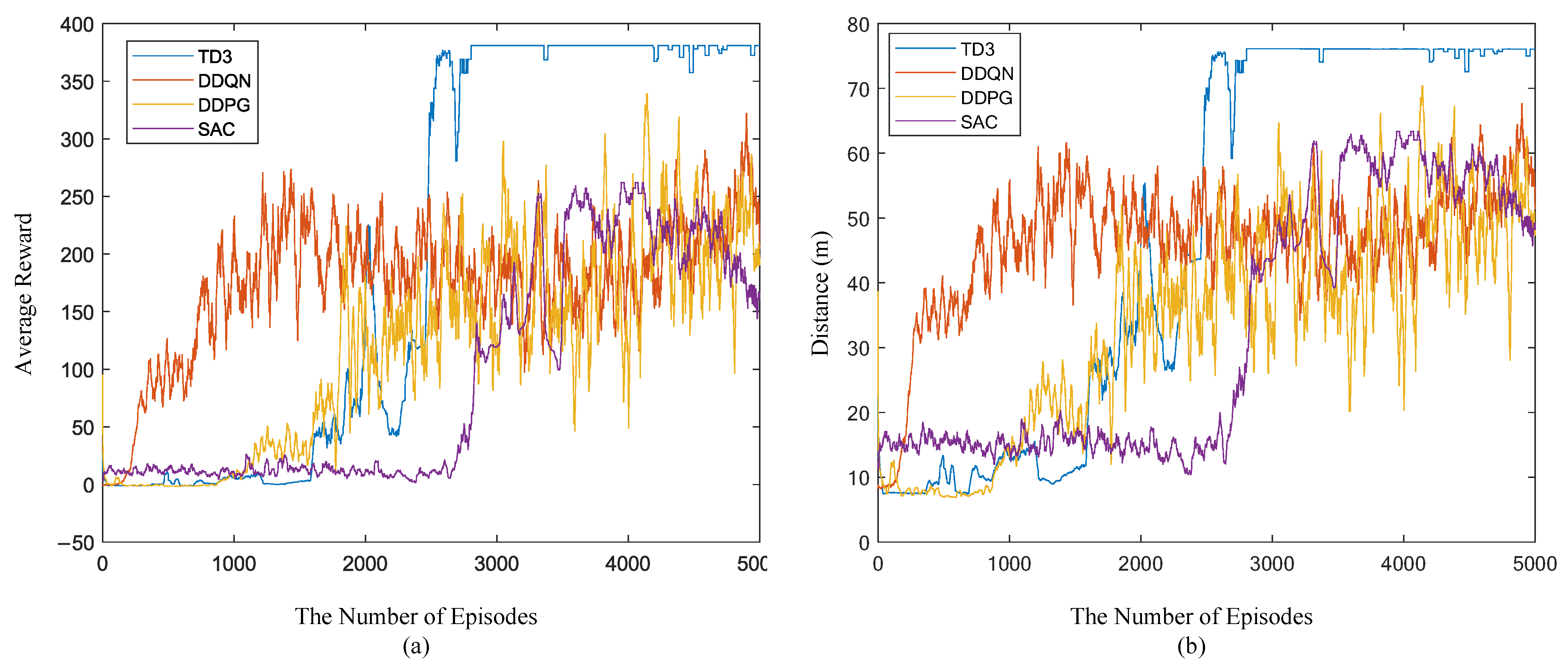
This paper proposes a reinforcement learning-based framework of STTW robot path planning, trajectory tracking, and balance control. The framework not only uses TD3 as the training algorithm for the agent, but also other reinforcement learning algorithms. For example, DDQN [14], DDPG [19], and SAC [26] can be used as training algorithms for our framework. The DDQN is a reinforcement learning algorithm based on the value function, which requires the action value output by the agent to be discrete. Therefore, we define the output of the DDQN as 11 actions that range from −10 N to 10 N, and we set an action every 2 N. The network used by the DDQN is consistent with the critic network in this article, and the actor and critic networks used by the DDPG algorithm are consistent with the network structure in our method. SAC is a reinforcement learning algorithm that computes an optimal policy that maximizes the policy’s long-term expected reward, as well as its entropy. Its critic networks are consistent with the networks used in this article, and its actor network adds the soft plus layer. The comparison results of the simulation are shown in Figure 16. As can be seen from Figure 16a, TD3 has the fastest training speed and is relatively stable after convergence. From Figure 16b, it can be seen that after TD3′s 2805th training episode, the robot can pass the entire runway.

5.5. Comparison between Different Reward Functions

This article proposes a reward function that allows STTW robots to complete narrow terrain passing tasks. To discuss the effect of this reward function, we conducted comparative training on different reward functions. The reward function for the comparison is as follows:
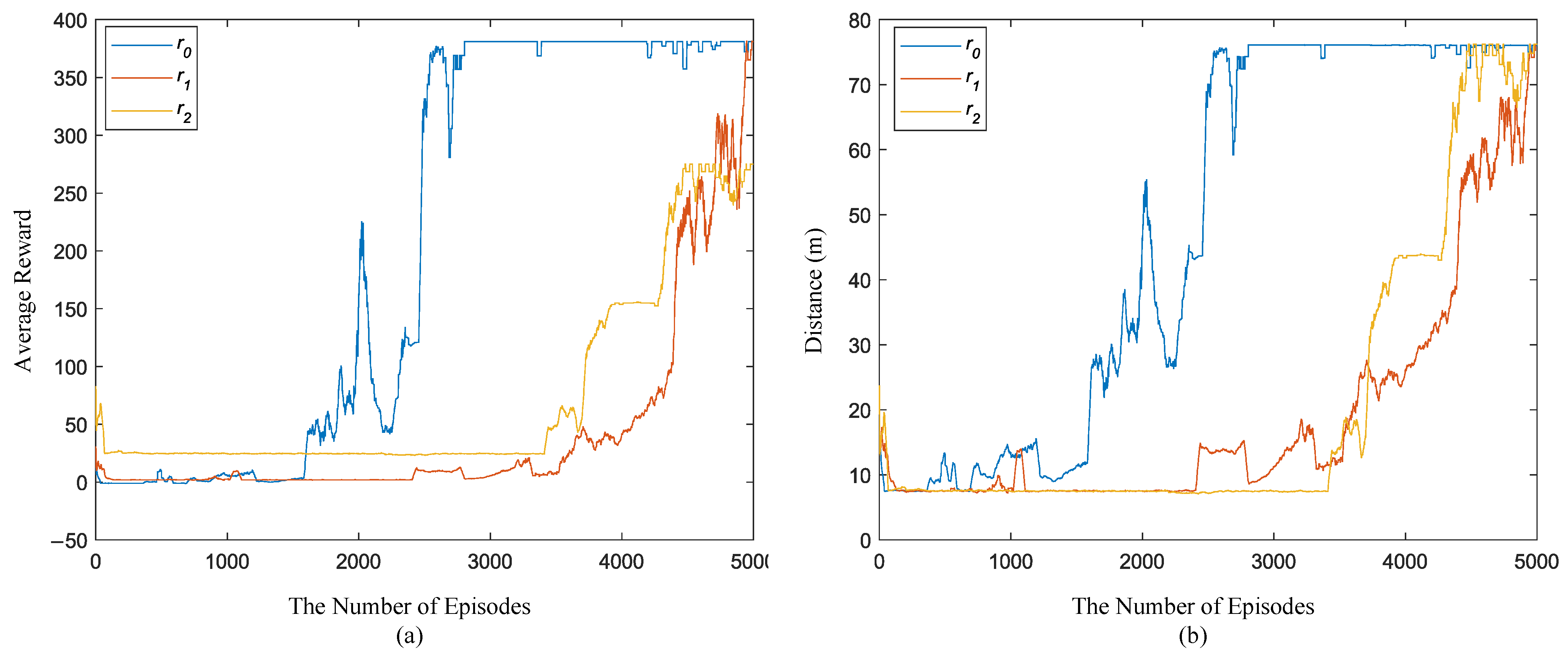
r 0 = C 1 C 2 ,
r 1 = C 1 ,
r 2 = 1 C 2 ,
where C1 and C2 are the same as those in Section 4.3. The comparison results are shown in Figure 17, where r0 represents the reward function used in Section 4. It can be seen from Figure 17a that this reward function converges faster than other reward value functions. It can be seen from Figure 17b that r1 and r2 completed the task of passing through narrow terrain at the end of training.

5.6. Comparison between Different Training Parameters

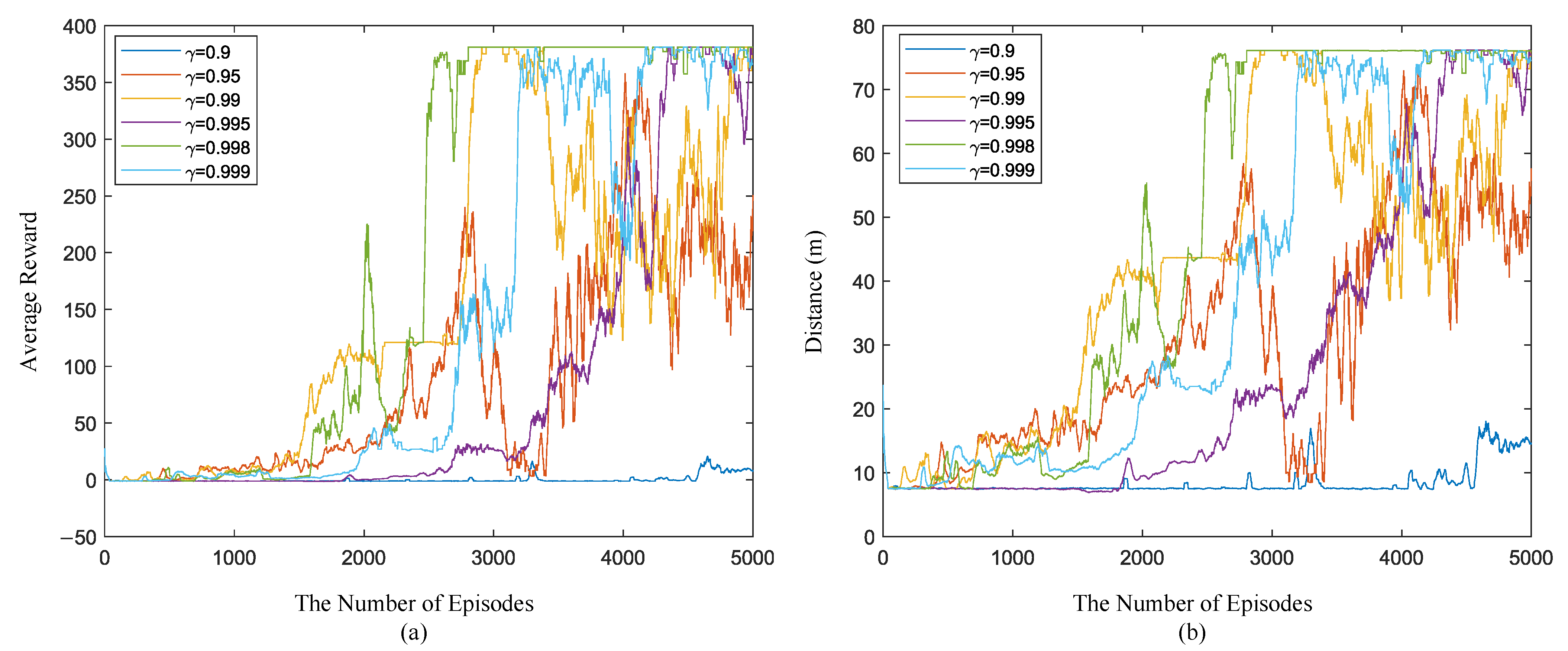
The discount factor γ is an important parameter in reinforcement learning. In our research, different γs were compared, and the comparison results are shown in Figure 18. When γ was set to 0.995, 0.998, and 0.999, the reward function could converge, but when γ was 0.998, the reward function was more stable after convergence.

6. Conclusions

In this article, we proposed an STTW robot control method to adapt to narrow terrain with limited visibility and line-of-sight occlusions. This control method integrates STTW robot path planning, trajectory tracking, and balance control in one framework. First, we defined the state and action according to the framework of reinforcement learning and designed a reward function that is effective for narrow terrain tasks. We also conducted comparative training to verify the effectiveness of the reward function. Second, according to the defined state, we designed the reward function, the actor network structure, and the critic networks structure. Then, we used the TD3 algorithm to train these neural networks and constructed a controller for the STTW robot. The comparative training results show that using TD3 results in a faster training speed than other reinforcement learning algorithms. Finally, we tested the trained controller and verified that it can perform well when tasked with passing through different narrow terrains. This paper compares the proposed method with traditional APF, RRT*, and the method in [46], and the results show that the proposed method can adapt to more types of terrain. Our results cast a new light on control methods for STTW robots.
STTW robots should be explored in future research. Firstly, the control method proposed in this article can be applied on a wider scale, especially to more complex narrow terrain. In addition, it can also be applied to the STTW robot ramp jump task. Secondly, future research could improve the physical prototype for the STTW robot and combine the reinforcement learning control method proposed in this article with transfer learning to enhance the STTW robot’s performance.

Author Contributions

Conceptualization, Q.Z. and Z.C.; methodology, Q.Z.; software, Q.Z. and Y.T.; validation, Q.Z., Y.T. and Y.D.; formal analysis, Q.Z.; writing—original draft preparation, Q.Z.; writing—review and editing, Y.D., Z.C. and X.Z.; supervision, B.L.; project administration, Z.C.; funding acquisition, Z.C. All authors have read and agreed to the published version of the manuscript.

Funding

This work was supported in part by National Natural Science Foundation of China (No. 62073183).

Institutional Review Board Statement

Not applicable.

Informed Consent Statement

Not applicable.

Data Availability Statement

The data presented in this study are available on request from the first author.

Conflicts of Interest

The authors declare no conflict of interest.

Appendix A

Table A1. Execution time for the evaluation process.
TerrainCompletedSimulation TimeExecution Time
Training Terrain11 s17.26 s
Test Terrain 120 s44.99 s
Test Terrain 213 s26.71 s
Test Terrain 316 s36.29 s
Test Terrain 415 s29.38 s

References

  1. Astrom, K.J.; Klein, R.E.; Lennartsson, A. Bicycle dynamics and control: Adapted bicycles for education and research. IEEE Control. Syst. Mag. 2005, 25, 26–47. [Google Scholar]
  2. Tanaka, Y.; Murakami, T. A study on straight-line tracking and posture control in electric bicycle. IEEE Trans. Ind. Electron. 2009, 56, 159–168. [Google Scholar] [CrossRef]
  3. Sun, Y.; Zhao, H.; Chen, Z.; Zheng, X.; Zhao, M.; Liang, B. Fuzzy model-based multi-objective dynamic programming with modified particle swarm optimization approach for the balance control of bicycle robot. IET Control. Theory Appl. 2022, 16, 7–19. [Google Scholar] [CrossRef]
  4. Suryanarayanan, S.; Tomizuka, M.; Weaver, M. System dynamics and control of bicycles at high speeds. In Proceedings of the 2002 American Control Conference, Anchorage, AK, USA, 8–10 May 2002. [Google Scholar]
  5. Yu, Y.; Zhao, M. Steering control for autonomously balancing bicycle at low speed. In Proceedings of the 2018 IEEE International Conference on Robotics and Biomimetics (ROBIO), Kuala Lumpur, Malaysia, 12–15 December 2018. [Google Scholar]
  6. Zhang, Y.; Li, J.; Yi, J.; Song, D. Balance control and analysis of stationary riderless motorcycles. In Proceedings of the 2011 IEEE International Conference on Robotics and Automation, Shanghai, China, 9–13 May 2011. [Google Scholar]
  7. Keo, L.; Yamakita, M. Control of an autonomous electric bicycle with both steering and balancer controls. Adv. Robot. 2011, 25, 1–22. [Google Scholar] [CrossRef]
  8. Yetkin, H.; Kalouche, S.; Vernier, M.; Colvin, G.; Redmill, K.; Ozguner, U. Gyroscopic stabilization of an unmanned bicycle. In Proceedings of the 2014 American Control Conference, Portland, OR, USA, 4–6 June 2014. [Google Scholar]
  9. Stasinopoulos, S.; Zhao, M.; Zhong, Y. Human behavior inspired obstacle avoidance & road surface quality detection for autonomous bicycles. In Proceedings of the 2015 IEEE International Conference on Robotics and Biomimetics (ROBIO), Zhuhai, China, 6–9 December 2015. [Google Scholar]
  10. Mnih, V.; Kavukcuoglu, K.; Silver, D.; Rusu, A.A.; Veness, J.; Bellemare, M.G.; Graves, A.; Riedmiller, M.; Fidjeland, A.K.; Ostrovski, G. Human-level control through deep reinforcement learning. Nature 2015, 518, 529–533. [Google Scholar] [CrossRef]
  11. Goodfellow, I.; Bengio, Y.; Courville, A. Deep Learning; MIT Press: Cambridge, MA, USA, 2016. [Google Scholar]
  12. Watkins, C.J.; Dayan, P. Q-learning. Mach. Learn. 1992, 8, 279–292. [Google Scholar] [CrossRef]
  13. Lin, L.-J. Self-improving reactive agents based on reinforcement learning, planning and teaching. Mach. Learn. 1992, 8, 293–321. [Google Scholar] [CrossRef]
  14. Van Hasselt, H.; Guez, A.; Silver, D. Deep reinforcement learning with double q-learning. In Proceedings of the AAAI Conference on Artificial Intelligence, Phoenix, AZ, USA, 12–17 February 2016. [Google Scholar]
  15. Silver, D.; Lever, G.; Heess, N.; Degris, T.; Wierstra, D.; Riedmiller, M. Deterministic policy gradient algorithms. In Proceedings of the International Conference on Machine Learning, Beijing, China, 21–26 June 2014. [Google Scholar]
  16. Peters, J.; Schaal, S. Natural actor-critic. Neurocomputing 2008, 71, 1180–1190. [Google Scholar] [CrossRef]
  17. Bhatnagar, S.; Sutton, R.S.; Ghavamzadeh, M.; Lee, M. Incremental Natural-Gradient Actor-Critic Algorithms. In Proceedings of the 21st Annual Conference on Neural Information Processing Systems, Vancouver, Canada, 3–6 December 2007. [Google Scholar]
  18. Degris, T.; White, M.; Sutton, R. Off-Policy Actor-Critic. In Proceedings of the International Conference on Machine Learning, Edinburgh, Scotland, 26 June–1 July 2012. [Google Scholar]
  19. Lillicrap, T.P.; Hunt, J.J.; Pritzel, A.; Heess, N.; Erez, T.; Tassa, Y.; Silver, D.; Wierstra, D. Continuous control with deep reinforcement learning. In Proceedings of the International Conference on Learning Representations (ICLR), San Juan, Puerto Rico, 2–4 May 2016. [Google Scholar]
  20. Barth-Maron, G.; Hoffman, M.W.; Budden, D.; Dabney, W.; Horgan, D.; Dhruva, T.; Muldal, A.; Heess, N.; Lillicrap, T. Distributed Distributional Deterministic Policy Gradients. In Proceedings of the 2018 International Conference on Learning Representations, Vancouver, BC, Canada, 30 April–3 May 2018. [Google Scholar]
  21. Vecerik, M.; Sushkov, O.; Barker, D.; Rothörl, T.; Hester, T.; Scholz, J. A practical approach to insertion with variable socket position using deep reinforcement learning. In Proceedings of the 2019 International Conference on Robotics and Automation (ICRA), Montreal, QC, Canada, 20–24 May 2019. [Google Scholar]
  22. Hausknecht, M.; Stone, P. Deep reinforcement learning in parameterized action space. In Proceedings of the 4th International Conference on Learning Representations (ICLR), San Juan, Puerto Rico, 2–4 May 2016. [Google Scholar]
  23. Fujimoto, S.; Hoof, H.; Meger, D. Addressing function approximation error in actor-critic methods. In Proceedings of the 35th International Conference on Machine Learning, Stockholm, Sweden, 10–15 July 2018. [Google Scholar]
  24. Schulman, J.; Levine, S.; Abbeel, P.; Jordan, M.; Moritz, P. Trust region policy optimization. In Proceedings of the 32nd International Conference on Machine Learning, Lille, France, 6–11 June 2015. [Google Scholar]
  25. Vanvuchelen, N.; Gijsbrechts, J.; Boute, R. Use of proximal policy optimization for the joint replenishment problem. Comput. Ind. 2020, 119, 103239. [Google Scholar] [CrossRef]
  26. Haarnoja, T.; Zhou, A.; Abbeel, P.; Levine, S. Soft actor-critic: Off-policy maximum entropy deep reinforcement learning with a stochastic actor. In Proceedings of the 35th International Conference on Machine Learning, Stockholm, Sweden, 10–15 July 2018. [Google Scholar]
  27. Choi, S.; Le, T.P.; Nguyen, Q.D.; Layek, M.A.; Lee, S.; Chung, T. Toward self-driving bicycles using state-of-the-art deep reinforcement learning algorithms. Symmetry 2019, 11, 290. [Google Scholar] [CrossRef] [Green Version]
  28. Zhu, X.; Deng, Y.; Zheng, X.; Zheng, Q.; Liang, B.; Liu, Y. Online Reinforcement-Learning-Based Adaptive Terminal Sliding Mode Control for Disturbed Bicycle Robots on a Curved Pavement. Electronics 2022, 11, 3495. [Google Scholar] [CrossRef]
  29. Guo, L.; Chen, Z.; Song, Y. Semi-empirical dynamics modeling of a bicycle robot based on feature selection and RHONN. Neurocomputing 2022, 511, 448–461. [Google Scholar] [CrossRef]
  30. Beznos, A.; Formal’Sky, A.; Gurfinkel, E.; Jicharev, D.; Lensky, A.; Savitsky, K.; Tchesalin, L. Control of autonomous motion of two-wheel bicycle with gyroscopic stabilisation. In Proceedings of the 1998 IEEE International Conference on Robotics and Automation, Leuven, Belgium, 20–20 May 1998. [Google Scholar]
  31. Wang, P.; Yi, J.; Liu, T. Stability and control of a rider–bicycle system: Analysis and experiments. IEEE Trans. Autom. Sci. Eng. 2019, 17, 348–360. [Google Scholar] [CrossRef]
  32. Seekhao, P.; Tungpimolrut, K.; Parnichkun, M. Development and control of a bicycle robot based on steering and pendulum balancing. Mechatronics 2020, 69, 102386. [Google Scholar] [CrossRef]
  33. Hwang, C.-L.; Wu, H.-M.; Shih, C.-L. Fuzzy sliding-mode underactuated control for autonomous dynamic balance of an electrical bicycle. IEEE Trans. Control. Syst. Technol. 2009, 17, 658–670. [Google Scholar] [CrossRef]
  34. Mu, J.; Yan, X.-G.; Spurgeon, S.K.; Mao, Z. Generalized regular form based SMC for nonlinear systems with application to a WMR. IEEE Trans. Ind. Electron. 2017, 64, 6714–6723. [Google Scholar] [CrossRef] [Green Version]
  35. Kim, Y.; Kim, H.; Lee, J. Stable control of the bicycle robot on a curved path by using a reaction wheel. J. Mech. Sci. Technol. 2015, 29, 2219–2226. [Google Scholar] [CrossRef]
  36. Chen, L.; Liu, J.; Wang, H.; Hu, Y.; Zheng, X.; Ye, M.; Zhang, J. Robust control of reaction wheel bicycle robot via adaptive integral terminal sliding mode. Nonlinear Dyn. 2021, 104, 2291–2302. [Google Scholar] [CrossRef]
  37. Elbanhawi, M.; Simic, M. Sampling-based robot motion planning: A review. IEEE Access 2014, 2, 56–77. [Google Scholar] [CrossRef]
  38. Karaman, S.; Frazzoli, E. Sampling-based algorithms for optimal motion planning. Int. J. Robot. Res. 2011, 30, 846–894. [Google Scholar] [CrossRef] [Green Version]
  39. Zhao, M.; Stasinopoulos, S.; Yu, Y. Obstacle detection and avoidance for autonomous bicycles. In Proceedings of the 2017 13th IEEE Conference on Automation Science and Engineering (CASE), Xi’an, China, 20–23 August 2017. [Google Scholar]
  40. Wang, P.; Yi, J.; Liu, T.; Zhang, Y. Trajectory tracking and balance control of an autonomous bikebot. In Proceedings of the 2017 IEEE International Conference on Robotics and Automation (ICRA), Singapore, 29 May–3 June 2017. [Google Scholar]
  41. Persson, N.; Ekström, M.C.; Ekström, M.; Papadopoulos, A.V. Trajectory tracking and stabilisation of a riderless bicycle. In Proceedings of the 2021 IEEE International Intelligent Transportation Systems Conference (ITSC), Indianapolis, IN, USA, 19–22 September 2021. [Google Scholar]
  42. He, K.; Deng, Y.; Wang, G.; Sun, X.; Sun, Y.; Chen, Z. Learning-Based Trajectory Tracking and Balance Control for Bicycle Robots With a Pendulum: A Gaussian Process Approach. IEEE/ASME Trans. Mechatron. 2022, 27, 634–644. [Google Scholar] [CrossRef]
  43. Lee, T.-C.; Polak, J.W.; Bell, M.G. BikeSim User Manual Version 1.0; Working paper; Centre for Transport Studies: London, UK, 2008. [Google Scholar]
  44. Dabladji, M.E.-H.; Ichalal, D.; Arioui, H.; Mammar, S. Unknown-input observer design for motorcycle lateral dynamics: Ts approach. Control. Eng. Pract. 2016, 54, 12–26. [Google Scholar] [CrossRef] [Green Version]
  45. Damon, P.-M.; Ichalal, D.; Arioui, H. Steering and lateral motorcycle dynamics estimation: Validation of Luenberger LPV observer approach. IEEE Trans. Intell. Veh. 2019, 4, 277–286. [Google Scholar] [CrossRef] [Green Version]
  46. Ryou, G.; Tal, E.; Karaman, S. Multi-fidelity black-box optimization for time-optimal quadrotor maneuvers. Int. J. Robot. Res. 2021, 40, 1352–1369. [Google Scholar] [CrossRef]
  47. Sharp, R.; Evangelou, S.; Limebeer, D.J. Advances in the modelling of motorcycle dynamics. Multibody Syst. Dyn. 2004, 12, 251–283. [Google Scholar] [CrossRef] [Green Version]
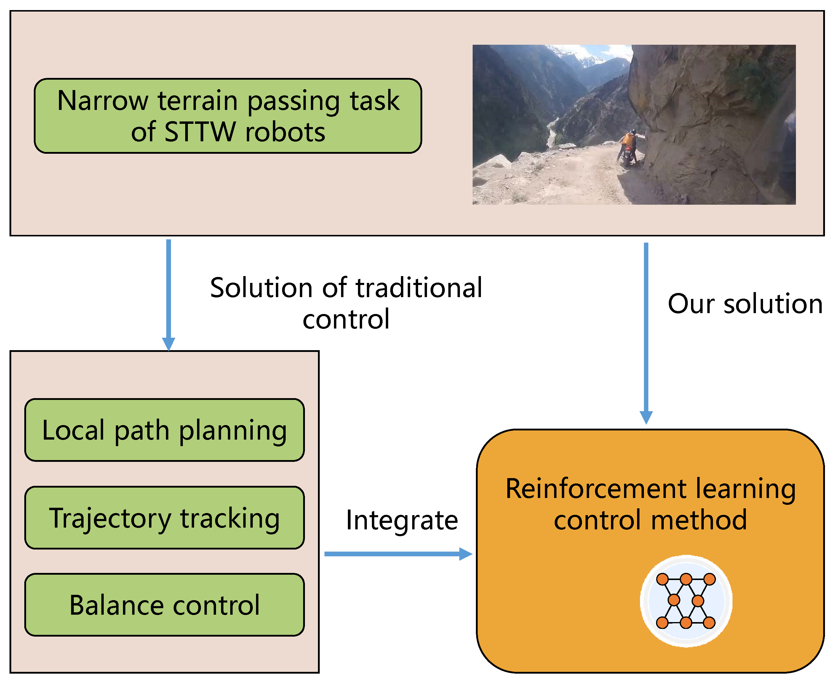
Figure 1. Solution for the narrow terrain passing task of the STTW robots.
Actuators 12 00109 g001
Figure 2. State sA settings.
Actuators 12 00109 g002
Figure 3. System coordinates.
Actuators 12 00109 g003
Figure 4. Network structure: (a) actor network; (b) critic network.
Actuators 12 00109 g004
Figure 5. The framework of the STTW robots reinforcement learning control method.
Actuators 12 00109 g005
Figure 6. Simulation platform.
Actuators 12 00109 g006
Figure 7. Terrain structure.
Actuators 12 00109 g007
Figure 8. Results of STTW robot driving on narrow terrain: (a) front wheel trajectory; (b) steering angle; (c) roll angle; (d) yaw angle; (e) steering torque.
Actuators 12 00109 g008
Figure 9. Results of STTW robot driving on straight-line terrain: (a) front wheel trajectory; (b) steering torque.
Actuators 12 00109 g009
Figure 10. Test terrain used for validation: (a) test terrain 1; (b) test terrain 2; (c) test terrain 3; (d) test terrain 4.
Actuators 12 00109 g010
Figure 11. The process of line-of-sight occlusions in state sA.
Actuators 12 00109 g011
Figure 12. Trajectories of the STTW robot in test scenario I: (a) training terrain; (b) test terrain 1; (c) test terrain 2; (d) test terrain 3; (e) test terrain 4.
Actuators 12 00109 g012
Figure 13. Trajectories of the STTW robot in test scenario II: (a) training terrain; (b) test terrain 1; (c) test terrain 2; (d) test terrain 3; (e) test terrain 4.
Actuators 12 00109 g013
Figure 14. Trajectories of the STTW robot in test scenario III: (a) training terrain; (b) test terrain 1; (c) test terrain 2; (d) test terrain 3; (e) test terrain 4.
Actuators 12 00109 g014
Figure 15. Trajectories using traditional method: (a) training terrain; (b) test terrain 1; (c) test terrain 2; (d) test terrain 3; (e) test terrain 4.
Actuators 12 00109 g015
Figure 16. Comparison between different reinforcement learning control methods: (a) average reward of the last 30 episodes in the training process; (b) average maximum distance of the last 30 episodes.
Actuators 12 00109 g016
Figure 17. Comparison between different reward functions: (a) average reward of the last 30 episodes in the training process; (b) average maximum distance of the last 30 episodes.
Actuators 12 00109 g017
Figure 18. Comparison between different training parameters: (a) average reward of the last 30 episodes in the training process; (b) average maximum distance of the last 30 episodes.
Actuators 12 00109 g018
Table 1. Relationship between the contents of the references and the proposition of this paper.
ContentLiterature
Refs. [1,3,4,5,6,8,27,31,32,33,36]Refs. [2,7,30,35,40,41,42]Refs. [37,38]Refs. [9,39]Refs. [28,29]
Path planning×××
Trajectory tracking×××
Balance control×
Consider narrow roads?××××
Consider uneven roads?××××
Consider low visibility?×××××
Consider line-of-sight occlusions?××××
Table 2. Comparison with traditional planning and control methods.
TerrainOur MethodAPFThe Method in [46]RRT*
Completed K r i d Completed K r i d Completed K r i d Completed
Training Terrain999
Test Terrain 165.55.5
Test Terrain 2999
Test Terrain 32.5×4.5×5×
Test Terrain 47×7×7×
Disclaimer/Publisher’s Note: The statements, opinions and data contained in all publications are solely those of the individual author(s) and contributor(s) and not of MDPI and/or the editor(s). MDPI and/or the editor(s) disclaim responsibility for any injury to people or property resulting from any ideas, methods, instructions or products referred to in the content.