Bearing Fault Diagnosis Method Based on Adversarial Transfer Learning for Imbalanced Samples of Portal Crane Drive Motor

Abstract

Due to their unique structural design, portal cranes have been extensively utilized in bulk cargo and container terminals. The bearing fault of their drive motors is a critical issue that significantly impacts their operational efficiency. Moreover, the problem of imbalanced fault samples has a more pronounced influence on the application of novel fault diagnosis methods. To address this, the paper presents a new method called bidirectional gated recurrent domain adversarial transfer learning (BRDATL), specifically designed for imbalanced samples from portal cranes’ drive motor bearings. Initially, a bidirectional gated recurrent unit (Bi-GRU) is used as a feature extractor within the network to comprehensively extract features from both source and target domains. Building on this, a new Correlation Maximum Mean Discrepancy (CAMMD) method, integrating both Correlation Alignment (CORAL) and Maximum Mean Discrepancy (MMD), is proposed to guide the feature generator in providing domain-invariant features. Considering the real-time data characteristics of portal crane drive motor bearings, we adjusted the CWRU and XJTU-SY bearing datasets and conducted comparative experiments. The experimental results show that the accuracy of the proposed method is up to 99.5%, which is obviously higher than other methods. The presented fault diagnosis model provides a practical and theoretical framework for diagnosing faults in portal cranes’ field operation environments.

1. Introduction

Due to their unique structure, gantry cranes have been extensively utilized in the loading and unloading of bulk cargo and container terminals. With the automation and unmanned operation of wharves, there is an urgent need for condition detection and fault diagnosis of door cranes. Consequently, the fault diagnosis of door engines has garnered significant attention from numerous scholars. As a primary piece of equipment, the drive motor of a door crane operates under high loads and various working conditions for extended periods. Its rolling bearings are critical components that are susceptible to damage due to complex working conditions, continuous overload work, and changing operational circumstances [1]. Therefore, monitoring the health status of rolling bearings is exceptionally crucial.

The state of the portal crane drive motor’s bearing in the operational process is subject to continuous variability, leading to a sample imbalance problem in fault data. The issue of unbalanced fault data sampling in portal crane drive motor bearings is a prevalent challenge in the fault diagnosis of port mainstream equipment and holds universal applicability. The solution to this problem carries extensive reference value for fault diagnosis in port equipment. Simultaneously, due to the intricate working conditions, varying metal structures, and performance characteristics, as well as the differing installation accuracies of drive motor bearings for portal cranes, the fault diagnosis process possesses its own distinctiveness. Therefore, it becomes imperative to conduct specialized research on the problem of unbalanced data sampling related to bearing failures in portal crane drive motors, which encompasses both universality and particularity. With the progression of artificial intelligence technology, intelligent algorithms like deep learning have begun to find application in fault diagnosis, yielding promising results [2,3]. However, these diagnostic methods assume that both the training and testing data conform to the same distribution, a condition that could potentially be nonideal in diagnosing portal crane motor bearings.

Hence, the proposal to incorporate domain adaptation, specifically adversarial transfer learning [4], into cross-domain fault diagnosis has been put forth to transfer the fault diagnosis knowledge to the target machine for improved results. However, data-driven fault diagnosis methods based on data will be primarily influenced by different distributions of the training set and test set. Large-scale equipment in an industrial context will exhibit substantial differences in historical data due to changing working conditions. Thus, leveraging these discrepancies in historical data, we can efficiently build a cross-domain fault diagnosis model across varying operational conditions.

While these datasets encompass variations from different failure levels, environments, and working conditions, the machines and signal acquisition systems generating the data might be identical. However, the likelihood of equipment failure, such as that of a portal crane, in their daily working conditions could be much higher, making it near-impossible to encounter all failure situations and resulting in minimal data collection. To overcome this data collection challenge, alternative methods to obtain failure data can be employed, such as accumulating or producing historical failure data from analogous machines, conducting laboratory simulations, or constructing mathematical simulation models. These data still encapsulate information about the failures inherent to that type of machine or system, making them more suited for training fault diagnosis models and better aligned with the needs of data-driven fault diagnosis.

According to the actual needs of the portal crane drive motor bearing fault diagnosis, consider the fault sample imbalance as the core problem and the complexity and uncertainty of fault diagnosis based on sample imbalance. In this paper, we choose for the first time to take the sample data imbalance of portal crane drive motor bearings as the background, utilize the public dataset, and make relevant adjustments. This paper chooses to construct the bidirectional gated recurrent domain adversarial transfer learning (BRDATL) fault diagnosis model with a bidirectional gated recurrent unit (Bi-GRU) as the feature extractor for this study.

In this study, we employ an adversarial transfer learning-based fault diagnosis model for portal crane drive motor bearings, with the primary contributions as follows.

(1)

The BRDATL fault diagnosis framework is proposed for the first time, focusing on the unbalanced fault samples of portal crane drive motor bearings. This issue represents an urgent practical problem in door motor fault diagnosis and also holds significant academic importance in the field of detection technology. While some scholars have previously suggested a fault diagnosis model based on adversarial transfer learning, no research has been conducted specifically on diagnosing faults in door motor drive motor bearings.

(2)

Additionally, a new domain distance measurement method called the maximum mean difference method (CAMMD) is introduced in the domain classifier to account for variations in domain distribution under different working conditions. In this study, we adjust the ratio of fault data to normal data from Case Western Reserve University (CWRU) and Xi’an Jiaotong University-Sum Young Tech (XJTU-SY) bearing datasets according to the working condition of portal crane drive motor bearings. A comparative experiment is then conducted with seven existing adversarial transfer learning models. Results demonstrate that, compared to these existing methods, BRDATL exhibits superior diagnostic performance. From a practical application standpoint, our proposed BRDATL framework shows exceptional potential for more challenging and complex cross-domain fault diagnosis as well as addressing domain imbalance issues through simulation experiments using open datasets. These findings provide a viable theoretical foundation for subsequent experiments conducted within real-world operational environments involving portal cranes.

The remainder of this paper is structured as follows: Section 2 outlines the relevant literature, while Section 3 delves into the fundamental theoretical knowledge. Section 4 focuses on the methodology proposed in this paper; Section 5 conducts the related experiments; and Section 4 concludes with the outlook.

2. Literature Review

In this section, we survey existing studies pertinent to our paper. The relevant research can be broadly classified into four stages: investigations into traditional fault diagnosis methods, studies on conventional deep learning diagnostic methods, research into transfer learning-based fault diagnostic methods, and studies focusing on transfer learning fault diagnostic methods rooted in different equipment or simulation data.

2.1. Traditional Fault Diagnosis Methods

Traditional machine fault diagnosis methods are broadly classified into failure physics and data-driven models. The application of the failure physics model is limited in cases where environmental factors significantly influence the operational signals of machinery, such as the portal crane. Hence, data-driven models, which focus on changes in vibration signals during bearing operation, become more relevant. Several data-driven models have been proposed to assess the health status of bearings, including support vector machines (SVM) [5], relevance vector machines (RVM) [6], support vector regression (SVR) [7], and autoencoders (AE) [8]. Recently, hybrid approaches combining model-based and data-driven methods have gained attention. For instance, Zhou et al. [9] successfully integrated variable modal decomposition (VMD) with SVM for rolling bearing fault diagnosis. Similarly, Wang et al. [10] incorporated empirical modal decomposition (EMD) with SVR, further enhancing the model with a complementary partial noise-assisted method (CPNAM) to tackle the modal mixing problem. This innovation led to better recognition of early bearing fault signals. Li et al. [11] introduced a fault diagnosis model that combines the Harrow Hassidim Lloyd (HHL) algorithm from quantum computing with the LS-SVM algorithm from machine learning, culminating in a quantum least squares support vector machine (QSVM). Nonetheless, the effectiveness of these models is largely dependent on the performance of the regression estimators.

2.2. Traditional Deep Learning Diagnostic Methods

Deep neural networks have seen widespread use in fault diagnosis due to their strong feature extraction capabilities. Several researchers have effectively combined these methods. Liu et al. [12] harnessed the spatial processing ability of CNNs and the time series processing capability of gated recurrent units (GRU). Instead of manually extracting features, CNN was employed to adaptively extract practical features, while GRU was used to further learn the features processed by the CNN, realizing fault diagnosis. Chen et al. [13] developed an intricate model that combined a multi-scale CNN, an LSTM neural network, and a deep residual learning model for diagnosing rolling bearing faults. This model blended a comprehensive multi-scale CNN-LSTM module with a deep residual module. In a similar vein, Kumar et al. [14] utilized the complete ensemble empirical mode decomposition with adaptive noise (CEEMDAN) technique to generate enhanced signals. They then employed a hybrid model of LSTM and GRU for fault diagnosis. Guo et al. [15] suggested an end-to-end fault diagnosis technique that utilizes attentional CNN and bidirectional LSTM (BiLSTM) networks. Nonetheless, all these methods hinge on the premise that the training and testing data adhere to the same distribution. This assumption can lead to issues such as accuracy imbalance, decision boundary imbalance, and overfitting when performing fault diagnosis based on imbalanced samples.

2.3. Diagnostics Based on Transfer Learning

Domain adaptive neural networks (DaNN) [16] employ an unsupervised feature alignment method grounded in MMD. In a similar vein, a deep adaptation network (DAN) [17] uses a multi-kernel MMD (MK-MMD) to gauge the distributional differences between two domains. Ganin et al. [18] incorporated adversarial learning into transfer learning to build a domain adversarial neural network (DANN). Zhang et al. [19] developed a fault diagnosis method based on transfer learning, testing it on bearing diagnosis data with varying fault diameters and under different loads. However, the early stages of faults typically lack distinct signals, resulting in limited training data for early fault diagnosis, particularly within the realm of deep learning models. To counter this, Chen et al. [20] proposed a transfer learning method using CNN to enhance feature learning from limited fault data, leading to improved diagnostic results.

Nevertheless, the techniques above should focus more on reducing adaptive edge distribution and the conditional distribution bias between them, which restricts their real-world classification performance. Li et al. [21] proposed a fault diagnosis technique utilizing a domain-adaptive CNN based on central moment discrepancy (CMD). This method extracts features with similar distributions from two domains and diagnoses faults in unlabeled data. However, it overlooks the different feature distributions arising from varying degrees of faults within the same data domain.

By capitalizing on variations in historical data, effective models can be constructed for cross-domain fault diagnosis under diverse operational conditions. Cheng et al. [22] enhanced the adversarial transfer method with Wasserstein distance to improve diagnostic model performance under targeted operating conditions by reusing data from different speeds and loads. Zou et al. [23] suggested a deep convolutional Wasserstein adversarial network (DCWAN)-based fault transfer diagnostic model. This model remedies the lack of pre-adaptation of feature distribution difference metrics between different operating conditions by expanding the feature boundaries in the source domain with variance constraints. Tong et al. [24] refined pseudo-test labels using MMD and domain invariant clustering (DIC) after fast Fourier transform (FFT) processing, effectively identifying bearing faults under different operating conditions. However, these studies did not account for differences in machine operating conditions. Zhao et al. [25] used bi-directional gated recurrent units (Bi-GRU) and manifold embedded distribution alignment (MEDA) for capturing historical feature data. The auxiliary samples generated by Bi-GRU align with the distribution of unlabeled samples in the target domain. Similarly, Wang et al. [26] presented a new subdomain adaptive transfer learning network (SATLN) model to integrate subdomain and domain adaptation. They base their model on for-labeling learning corrections while reducing marginal and conditional distribution biases. While these studies account for differences from varying fault levels, environments, and operating conditions, realizing such differences remains challenging when identical machines and signal acquisition systems generate the data.

2.4. Diagnostics Based on Transfer Learning from Different Devices or Simulation Data

Utilizing fault data from other sources can provide more sample data for domain-adaptive learning and more comprehensively reflect the fault situation, thus improving fault diagnosis models’ performance and robustness. Based on the above ideas, some scholars have researched cross-domain fault diagnosis from datasets generated from different machines or data sources. Zhang et al. [27] presented a novel framework to address the issue of distinct bearing fault data in different oil wells. They considered the bearings from two oil wells as the source and target domains and computed the transformation matrix to shift these data into a shared low-dimensional subspace, wherein the source data incorporating all kinds of fault samples and the target data missing some fault types are represented by a joint dictionary matrix. They then proceeded with an extensive series of experiments. Han et al. [28], taking into account the comprehensive scenarios of multiple operating conditions and machines, centered their main approach around pairing source and target data under the same machine conditions. They then executed domain adaptation separately to mitigate the absence of target data, diminish distribution differences, and prevent negative transfer. As for the simulation data generation, Dong et al. [29] utilized the dynamic model of bearings to generate a large number of diverse simulation data, and then, based on the convolutional neural network (CNN) and parameter passing strategy, the diagnostic knowledge acquired from the simulation data were applied to the actual scenario. The method could acquire more transferable features, decrease the disparity in feature distribution, and considerably enhance fault recognition performance.

For the public laboratory simulation data sets, representative types include the CWRU bearing data set and the XJTU-SY bearing data set, among others. Ji et al. [30] proposed a two-stage algorithm for bearing fault diagnosis and conducted experiments on both the CWRU bearing data set and their own data sets. Under identical training data sets, this algorithm significantly enhances the diagnostic performance of deep Convolutional Neural Networks (DCNN) under time-domain variable velocity conditions. Zuo et al. [31] introduced a multi-layer spiking neural network (SNN) method for bearing fault diagnosis and validated its effectiveness using datasets from CWRU, MFPT, and Paderborn University. Yu et al. [32] presented a novel subclass Reconfiguration Network (SCRN) model for rotating machinery fault diagnosis and evaluated it on three public datasets: CWRU, 2009 PHM, and MFPT. The results consistently demonstrated that the proposed method outperforms existing state-of-the-art techniques in terms of diagnostic performance. Ding et al. [33] proposed an intelligent edge diagnosis method based on parameter transplantation in convolutional neural networks (CNN). Verification using the CWRU dataset revealed an average prediction accuracy of 94.4% on the test set with this approach. Ma et al. [34] developed a new multi-step dynamic slow feature analysis (MS-DSFA) algorithm and verified its universality using the XJTU-SY bearing dataset as evidence. Xu et al. [35] constructed a hybrid deep learning model based on CNNs and gcForest, evaluating its performance using experimental bearing data provided by CWRU and XJTU-SY. Maurya et al. [36] devised an intelligent health monitoring management scheme for rotating machinery, which was validated with aero-engine as well as XJTU-SY bearing datasets. According to the researchers, publicly available data sets collected from laboratory machines can be used to evaluate fault diagnosis algorithms.

Despite the feasibility of these data-driven methods for bearing fault diagnosis, they still face several challenges:

(1)

The probability of portal crane failure in daily production environments varies with working conditions, operating times, and operating ages. Therefore, troubleshooting the bearings of the drive motor of a portal crane based on a single situation has limitations.

(2)

Different operating conditions can induce variations in the distribution of vibration signals from the portal crane drive motor bearings. This can yield poor results when models trained under one operating condition are used to troubleshoot another.

(3)

Most methods assume an identical distribution between the training and test sets. However, portal crane drive motor bearings generate fewer fault data during operation, with most of the sample data derived under normal conditions. Thus, these methods often need to pay more attention to sample distribution differences.

Aiming at the above problems, this paper considers the working conditions of the portal crane drive motor. It reclassifies and sets up the bearing dataset disclosed by CWRU and XJTU-SY, so that the data are closer to the data generated by the bearings of the portal crane drive motor when it is working. Thus, the experiments are closer to the actual industrial environment. We also propose a novel BRDATL framework and conduct comparative experiments with seven other existing adversarial transfer learning models. This approach validates the efficacy of our adapted method in simulation experiments, providing a viable diagnostic ideal for subsequent experiments in the portal crane’s operational environment.

3. Theory Background

3.1. Bi-GRU Network for Feature Extraction

RNN is a deep learning model that learns recursively along the sequence evolution direction using sequence data as input. In the hidden layers of RNNS, neurons are interconnected. This feature allows data from all layers to be shared between neural nodes. Therefore, RNN has good performance in the analysis of time data. However, RNN updates network parameters using a backpropagation algorithm. In training, gradient disappearance or gradient explosion will occur if the extended sequence model needs to be processed. LSTM is an improved network of RNN that is used for long-term prediction and solves the above problems well. GRU is superior to LSTM in computational performance, and the two are similar in structure, so this paper chooses GRU as the component unit of the feature extractor.

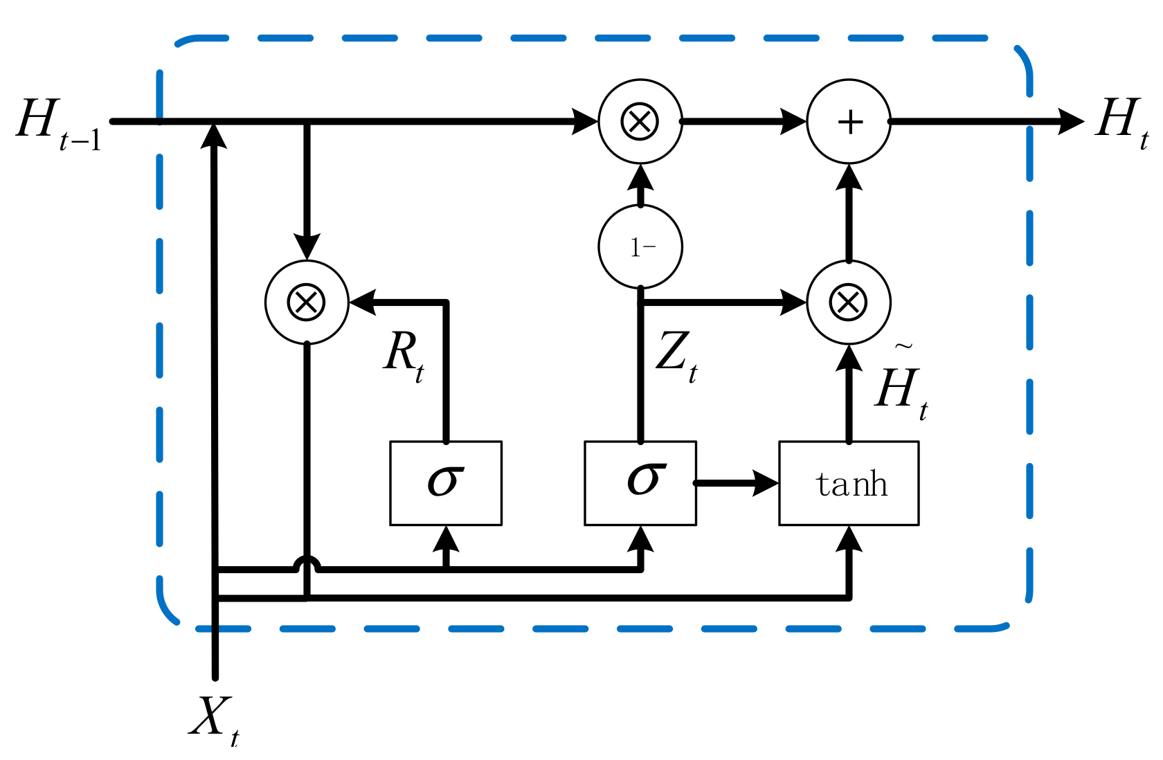
The GRU network mainly consists of a reset gate and an update gate, as shown in Figure 1. The key function of the reset gate is as follows: when it is near 1, the candidate hidden state information results from the multilayer perceptron consisting of both the input and the preceding state information. However, when the reset gate is near 0, the candidate hidden state is derived solely from the multilayer perceptron composed of the current inputs. The central role of the update gate is that when it is near 1, the model tends to retain only the previous state, disregarding the information from the inputs. Conversely, when the update gate is close to 0, the new hidden state tends to match the candidate hidden state.

The primary advantages of the GRU include its reset gate’s ability to capture short-term dependencies in the sequence effectively, thereby avoiding the vanishing gradient problem. Additionally, the update gate helps seize long-term dependencies within the sequence.

According to the above description, the reset gate for the current time step can be expressed as:

$${\mathbb{R}}_t=\sigma (X_t{\omega }_{xr}+{\stackrel{\rightharpoonup }{\rho }}_{t-1}{\omega }_{hr}+{\xi }_r)$$

(1)

where $X_t$ is the sample input at the current time, ${\stackrel{\rightharpoonup }{\rho }}_{t-1}$ denotes the current hidden state, ${\omega }_{xr}$, ${\omega }_{hr}$ are the weight parameters of the reset gate, and ${\xi }_r$ is the bias parameter of the reset gate.

Then, the update gate for the current timestep can be expressed as:

$$Z_t=\sigma (X_t{\omega }_{xz}+{\stackrel{\rightharpoonup }{\rho }}_{t-1}{\omega }_{hz}+{\xi }_z)$$

(2)

where ${\omega }_{xz}$, ${\omega }_{hz}$ are the weight parameters of the update gate and ${\xi }_z$ is the bias parameter of the update gate.

Integrating the reset gate ${\mathbb{R}}_t$ with the regular hidden state update mechanism yields the candidate hidden state $\widetilde{{\stackrel{\rightharpoonup }{\rho }}_t}$ at the time step $t$:

$$\widetilde{{\stackrel{\rightharpoonup }{\rho }}_t}=\tanh [X_t{\omega }_{xh}+({\mathbb{R}}_t\otimes {\stackrel{\rightharpoonup }{\rho }}_{t-1}){\omega }_{hh}+{\xi }_h]$$

(3)

where ${\omega }_{xh}$, ${\omega }_{hh}$ are weight parameters and ${\xi }_h$ is a bias parameter.

Finally, the new hidden state ${\stackrel{\rightharpoonup }{\rho }}_t$ can be derived for the time step $t$:

$${\stackrel{\rightharpoonup }{\rho }}_t=Z_d\otimes {\stackrel{\rightharpoonup }{\rho }}_t{}_{-1}+(1-Z_d)\otimes \widetilde{{\stackrel{\rightharpoonup }{\rho }}_t}$$

(4)

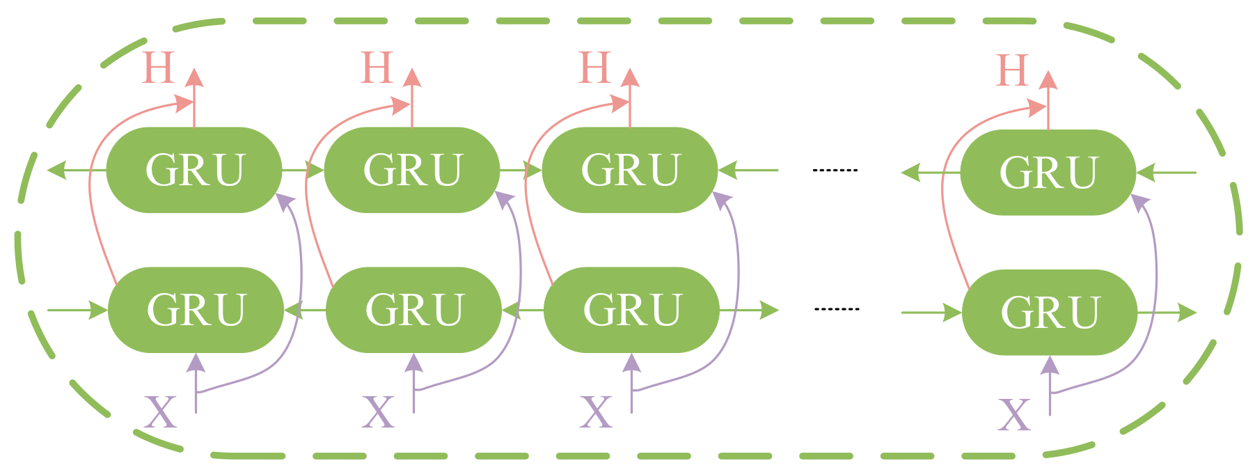
In this paper, we consider using Bi-GRU as the feature extractor for the model. Bi-GRU consists of two GRUs, forward and reverse, which can extract the feature information of the past and the future at the same time. The output of the Bi-GRU is determined by the hidden states of the two GRUs. The structure of the Bi-GRU is shown in Figure 2. Similarly, we can derive the output of reverse GRU as ${\stackrel{\leftharpoonup }{\rho }}_t$ and finally, we can derive the output of Bi-GRU as ${\stackrel{\rightharpoonup }{\rho }}_t+{\stackrel{\leftharpoonup }{\rho }}_t$.

3.2. BRDATL

GAN is a new model proposed by Goodfellow [37]. During adversarial training, two models compete: the generator and the discriminator. Generator G aims to deceive discriminator D to maximize the classification error. Discriminator D measures the distance between the actual PR and the generated PZ.

In the domain adaptation challenge, a domain is generally defined as comprising a feature space X and a marginal probability distribution P(X). It typically includes a source domain and a target domain. Compared to GAN, the domain adaptation problem eliminates the process of sample generation, treating the data in the target domain as generated samples directly. Traditional domain adaptation problems usually opt for fixed features, but the adversarial transfer network concentrates on determining which features can be transferred between different domains effectively. 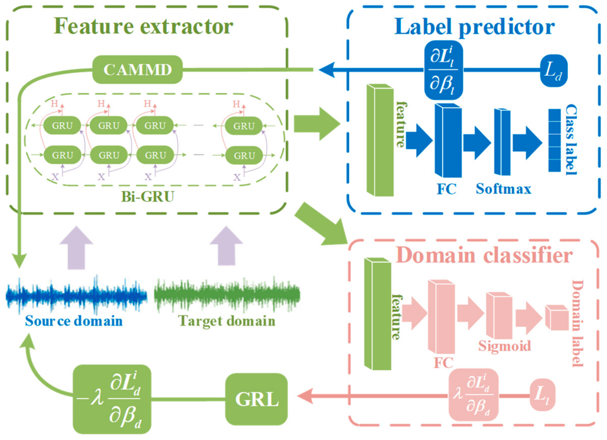Figure 3 shows the network diagram of BRDATL in this paper.

The feature extractor is in the green part of Figure 3. This approach maps and blends samples from the source domain with those from the target domain, causing the domain classifier to be unable to discern the origin of the data. It extracts the necessary features for the subsequent network to perform the task, enabling the label predictor to distinguish the class of data from the source domain. Aiming at the special working conditions of the door crane, this paper introduces the Bi-GRU mentioned in 3.1 as the feature extractor of the network, which can better extract the historical state information of the door crane when the working conditions change.

Then, the feature extractor ${\Phi }_f$ can be defined as:

$${\Phi }_f(X)=F_{B\mathrm{i}GRU}\left(X\right)$$

(5)

where $X$ is the actual input vector, which includes source domain samples $X_S$ and target domain sample $X_T$ data.

To generalize the model to real data ${\Phi }_f(;{\beta }_f)$ it can be used as a feature extractor for a $B$ dimensional neural network, and ${\beta }_f$ is the set of weights and bias parameters for the network.

The label predictor ${\Phi }_l$ is the blue part in Figure 3. Its primary role is to map the input data to the corresponding category labels according to the high-level features learned by the feature extractor, and the label predictor is responsible for accomplishing the classification task. Like the feature extractor, the label predictor ${\Phi }_l$ can be defined as:

$$\begin{array}{l}{\Phi }_l({\Phi }_f(x);{\omega }_l,{\xi }_l)=soft\max ({\omega }_l{\Phi }_f(x)+{\xi }_l)\\ ={\displaystyle \sum _{i=1}^c\left[\raisebox{1ex}{$\exp ({\omega }_l{\Phi }_f(x)+{\xi }_l)$}\!\left/ \!\raisebox{-1ex}{${\displaystyle \sum _{j=1}^c\exp ({\omega }_l{\Phi }_f(x)+{\xi }_l)}$}\right.\right]}\end{array}$$

(6)

where ${\omega }_l$ and ${\xi }_l$ are the weight parameter and bias parameter of the label predictor with sizes $c\times B$ and $c$, respectively.

The domain classifier ${\Phi }_d$ is in the red part of Figure 3 and classifies data in feature space, attempting to discern the origin of the data as accurately as possible. It takes the features extracted by the feature extractor as input and endeavors to classify these features into their respective domains. By training the domain classifier, we can make the features generated by the feature extractor insensitive to domain information, thus making the model more generalized to the target domain. The domain classifier ${\Phi }_d$ can be represented as:

$$\begin{array}{l}{\Phi }_d({\Phi }_f(x);{\omega }_d,{\xi }_d)=sigmoid({\omega }_d^T{\Phi }_f(x)+{\xi }_d)\\ =\frac{1}{1+\exp [-({\omega }_d^T{\Phi }_f(x)+{\xi }_d)]}\end{array}$$

(7)

where ${\omega }_d$ and ${\xi }_d$ are the weight parameter and bias parameter of the label predictor with sizes $c\times B$ and $c$, respectively.

3.3. Challenges of Class Imbalance

Many scholars have studied the class imbalance problem, and the critical aspect of solving this problem lies in solving the problem of the large gap between various intelligent learning algorithms and the desired positive performance on a dataset with an unbalanced distribution of fault categories. In traditional algorithms, it is generally assumed that each fault category of each data sample contributes equally to the decision analysis, and an attempt is made to solve this problem by training classifiers with cross-entropy loss. However, in this case, the overfitting problem will result since the dominant category completely dominates the classifier’s training.

There are two main directions for the solution to the class imbalance problem. One is to resample the minor classes or generate pseudo-samples of a few samples before training. The other is to relax the above assumptions by using cost-sensitive reweighting during training. However, each of these methods has its advantages and disadvantages. Method 1 will perform repeated preprocessing on the same samples, which will reduce the training speed of the network and make the model overfit, thus failing to achieve the desired accuracy. In contrast, class-balanced learning through cost-sensitive reweighting method 2 aims to redistribute the weights of the samples based on a given data distribution and provide all classes with equal opportunities to impact the loss function during training. With the reweighting strategy, the learned classifier’s decision boundary can remain balanced between large and small classes.

4. Method Mentioned

4.1. Fault Diagnosis Process for BRDATL

The most important thing for the fault diagnosis of industrial equipment is to find fault anomalies in time. Moreover, take corresponding measures before the failure or take timely reactions when the failure occurs to prevent equipment failures from causing more significant losses.

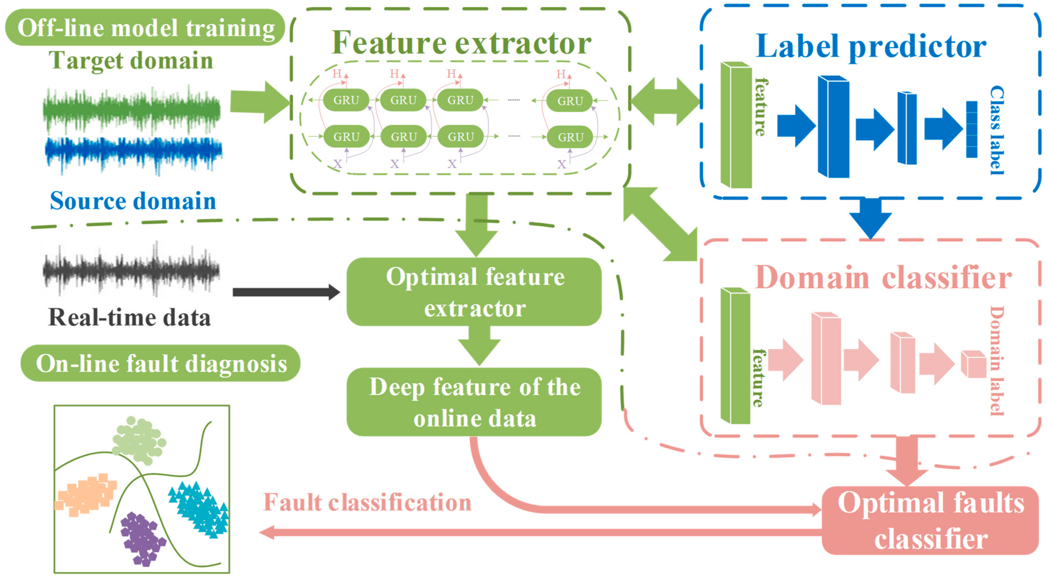
The BRDATL-based fault diagnosis proposed in this paper is mainly divided into two parts: offline training of the diagnostic model and online state detection. As shown in Figure 4, in the off-line part of the model training, the feature extractor Bi-GRU is first applied to the input signal feature extraction $F_{B\mathrm{i}GRU}\left(X\right)$, to obtain the depth of the signal feature, the feature is passed into the label predictor domain classifier. The domain classifier is responsible for creating an adversarial environment to determine whether the signal comes from the source domain or the target domain $F_{B\mathrm{i}GRU}\left(X\right)$, and this process is conducted through CAMMD. Then, the parameters of the feature extractor are updated through the gradient reverse layer GRL, so that the domain classifier cannot distinguish whether the parameters extracted by the feature extractor are from the source domain or the target domain. At the same time, the domain classifier is trained so that it can judge which domain the feature comes from and obtain the best feature extractor in this adversarial environment. The label predictor finally predicts the type of fault through $F_{B\mathrm{i}GRU}\left(X\right)$, updates the hyperparameters through cross-validation with the feature extractor, and finally becomes a more accurate fault classifier. Next is the online fault diagnosis process, where the real-time data are passed to the optimal fault classifier after the optimal feature extractor extracts the deep features, and the fault results are derived from the fault classifier in real-time.

4.2. Distance Measurement Based on CAMMD

In the domain adaptation problem, the distance between the source domain and the target domain is an important criterion, and some metrics have been proposed on the distance between the two domains. However, almost no method has absolute superiority. CORAL is an unsupervised feature alignment metric that calculates the second-order statistical difference between the source and target domains. It learns a nonlinear transformation that aligns layer activation correlations in a deep neural network. Similarly, MMD is extensively used in transfer learning. It can measure unsupervised feature alignment, drawing the features from the source and target domains closer together. Based on the above, a distance assessment method, CAMMD, is proposed for the first time. On the basis of CORAL alignment characteristics, MMD is used to further adapt.

First, consider a distributional difference metric to quantify the differences with other views to minimize the differences in the generated features between the two domains. For CORAL, make the following definitions:

$$M_S=\frac{1}{n_s-1}\left(X_s^T{X}_s-\frac{1}{n_s}{({\xi }_1^T{X}_s)}^T({\xi }_1^T{X}_s)\right)$$

(8)

$$M_T=\frac{1}{n_T-1}\left(X_T^T{X}_T-\frac{1}{n_T}{({\xi }_1^T{X}_T)}^T({\xi }_1^T{X}_T)\right)$$

(9)

where $n_s$ and $n_T$ are the number of samples, $M_S$ and $M_T$ are the feature covariance matrices. ${\xi }_1^{}$ is a column vector, which are all elements 1.

This leads to the definition of CORAL as:

$$F_{CORAL}\left(X_S,X_T\right)=\frac{1}{4d^2}\parallel M_s-M_T{\parallel }_F^2$$

(10)

where $\parallel •{\parallel }_F^2$ is the square matrix Frobenius paradigm.

In this study, MMD is also selected to further evaluate the disparity between the two domains, for which we provide the following definition:

$$F_{MMD}\left({\chi }_S,{\chi }_T\right)=\parallel \frac{1}{n_S}{\displaystyle \sum _{i=1}^{n_S}\varphi ({\left({\chi }_S\right)}_i)}-\frac{1}{n_T}{\displaystyle \sum _{j=1}^{n_T}\varphi ({\left({\chi }_T\right)}_j)}{\parallel }_H^2$$

(11)

where ${\chi }_S$, ${\chi }_T$ and are the features extracted by the feature extractor for the source and target domains, $\varphi (•)$ denotes the function mapped to the Hilbert space, and $\parallel •{\parallel }_H^2$ denotes the reproduction of the Hilbert space.

Hence, we can define CAMMD as follows:

$$F_{CAMMD}=F_{CORAL}\left(X_S,X_T\right)+F_{MMD}\left({\chi }_S,{\chi }_T\right)$$

(12)

Based on the above two metrics, the loss function $L_f$ of the feature extractor can be composed by CAMMD as follows:

$$L_f=F_{CAMMD}$$

(13)

4.3. Loss Function Optimization

For a source sample $\left(x_i,y_i\right)$, the loss of the label predictor in the source domain $L_l^S$ can be expressed as:

The loss of the label predictor in the target domain $L_l^T$ can be expressed as:

$$L_l^S=-\frac{1}{n}{\displaystyle \sum _{i=1}^n{L}_l({\Phi }_l({\Phi }_f(x_i)),y_i)}=-\frac{1}{n}{\displaystyle \sum _{i=1}^n\log [{\Phi }_l{({\Phi }_f(x_i))}_{y_i}]}$$

(14)

$$L_l^T=-\frac{1}{N-n}{\displaystyle \sum _{i=n+1}^N[{\Phi }_l{({\Phi }_f(x_i))}_{y_i}]\log [{\Phi }_l{({\Phi }_f(x_i))}_{y_i}]}$$

(15)

Similarly, ${\Phi }_l(;{\beta }_l)$ it can be used to compute the output of the label predictor for the whole network and ${\beta }_l$ is the set of weights and bias parameters for the output layer of the label predictor. Then, the first $i$ samples $\left(x_i,y_i\right)$, $L_l$ can be re-expressed as:

$$\begin{array}{l}{L}_l^{}=L_l^S+L_l^T\\ =-\frac{1}{n}{\displaystyle \sum _{i=1}^n\log [{\Phi }_l{({\Phi }_f(x_i;{\beta }_f);{\beta }_l)}_{y_i}]}\\ -\frac{1}{N-n}{\displaystyle \sum _{i=n+1}^N[{\Phi }_l{({\Phi }_f(x_i;{\beta }_f);{\beta }_l)}_{y_i}]}\\ \times {\displaystyle \sum _{i=n+1}^N\log [{\Phi }_l{({\Phi }_f(x_i;{\beta }_f);{\beta }_l)}_{y_i}]}\end{array}$$

(16)

The training process of adversarial networks is made more accessible due to the GRL introduced. The principle can be summarized as follows: In the BRDATL backpropagation process, the domain classifier predicts the domain class labels of the current sample, after which it backpropagates the error between its predictions and the actual domain class labels layer by layer. At each layer, the domain classifier computes the gradient based on the returned error. When the error reaches the gradient reversal layer, the output of the gradient inversion layer is multiplied by $-\lambda$, and this error is subsequently passed to the feature extractor. This allows the feature extractor to be trained with the exact opposite goal of the domain classifier, resulting in an adversarial effect. Thus, we can define GRL as follows:

$$G_{RL}(\Phi (x,\beta ),\lambda )=\Phi (x,\beta )$$

(17)

$$\frac{\partial }{\partial x}{G}_{RL}(\Phi (x,\beta ),\lambda )=-\lambda \frac{\partial }{\partial x}\Phi (x,\beta )$$

(18)

The domain classifier output can be expressed as follows:

$$d(x_i;{\beta }_d)={\Phi }_d(G_{RL}({\Phi }_f(x),\lambda );{\beta }_d)$$

(19)

Then, for the first $i$ samples $\left(x_i,z_i\right)$, $L_d$ can be re-expressed as:

$$\begin{array}{l}{L}_d^i=L_d(d(x_i;{\beta }_d),z_i)\\ =-\frac{1}{n}{\displaystyle \sum _{i=1}^n{z}_i\log [d(x_i;{\beta }_d)]}\\ -\frac{1}{N-n}{\displaystyle \sum _{i=n+1}^N(1-z_i)\log [1-d(x_i;{\beta }_d)]}\end{array}$$

(20)

In this paper, two constraint parameters $\mu$ and $\nu$ are introduced, respectively, to limit local optimization behavior and prevent training bias in label predictors and domain classifiers. Finally, the total loss of adversarial transfer training can be obtained as follows:

$$\begin{array}{l}L=L_f-L_D\\ =L_f-L_l^S-\mu L_l^T-\nu L_d^i\end{array}$$

(21)

Domain adaptation is integrated into the high-level feature learning process in training. Particularly, the feature extractor sequentially learns high-level features from two domains. Meanwhile, the classifier observes the difference between the continuously updated features. It utilizes adversarial training to minimize the difference between the two features by the backpropagation algorithm, and then the feature extractor learns the domain-invariant features. The BRDATL is summarized in Algorithm 1.

Algorithm 1 BRDATL for Fault Diagnosis in this study

Input: the original signal $S={(x_i,y_i)}_{i=1}^N$ from $X_S$ and $X_T$, number of batch sizes Batch-size, number of epochs Epochs, global equilibrium parameter [$\mu$, $\nu$], learning rate l, hyperparameters of loss calibration $\lambda$.

Output: the best feature extractor ${\Phi }_l$ and the best label predictor ${\Phi }_f$.

1. For epoch = 1 to Epochs:

2.  For batch = 1 to Batch-size:

3.    The sample $S={(x_i,y_i)}_{i=1}^N$ from $X_S$ and $X_T$     With the minimum batch size

4.    Forward propagation $S={(x_i,y_i)}_{i=1}^N$

5.    Calculate the classification loss $S={(x_i,y_i)}_{i=1}^N$ from $X_S$

6.     Calculate the sample size n of the relevant class

7.    Calibrate the loss and obtain $L_f$ by $\lambda$ and n

8.   Obtain $L_l$ and $L_d$ by inputting pseudo-labels to ${\Phi }_l$ and ${\Phi }_d$

9.    Calculate the total loss:       $L=L_f-L_l^S-\mu L_l^T-\nu L_d^i$

10.    Backward propagation $\lambda$ and GRL for ${\Phi }_d$

11.   Update ${\Phi }_f$, ${\Phi }_l$ and ${\Phi }_d$ by optimizer with learning rate l

12.  End

13. End

5. Experiments and Results

In this section, based on the rolling bearing vibration data collected by the rolling bearing fault simulation platform of the Electrical Engineering Laboratory of Case Western Reserve University (CWRU), the validity of the BRDATL proposed in this paper for the bearing fault diagnosis of the door drive motor is verified by adjusting the set sample number and mimicking the data that the door drive motor may produce in the actual industrial environment.

5.1. Experimental Platform

This experiment was conducted in PyCharm 2022.1.3 software on the win10 platform. The Pytorch framework was used for better results; GPU environment training was used; the GPU model is an RTX 3060 Laptop with 6 GB of memory and CUDA version 12.0; in addition, the CPU is an Intel i7-12700H, and the RAM size of the computer is 32 GB.

5.2. Introduction to the Dataset

(1)

CWRU-bearing dataset

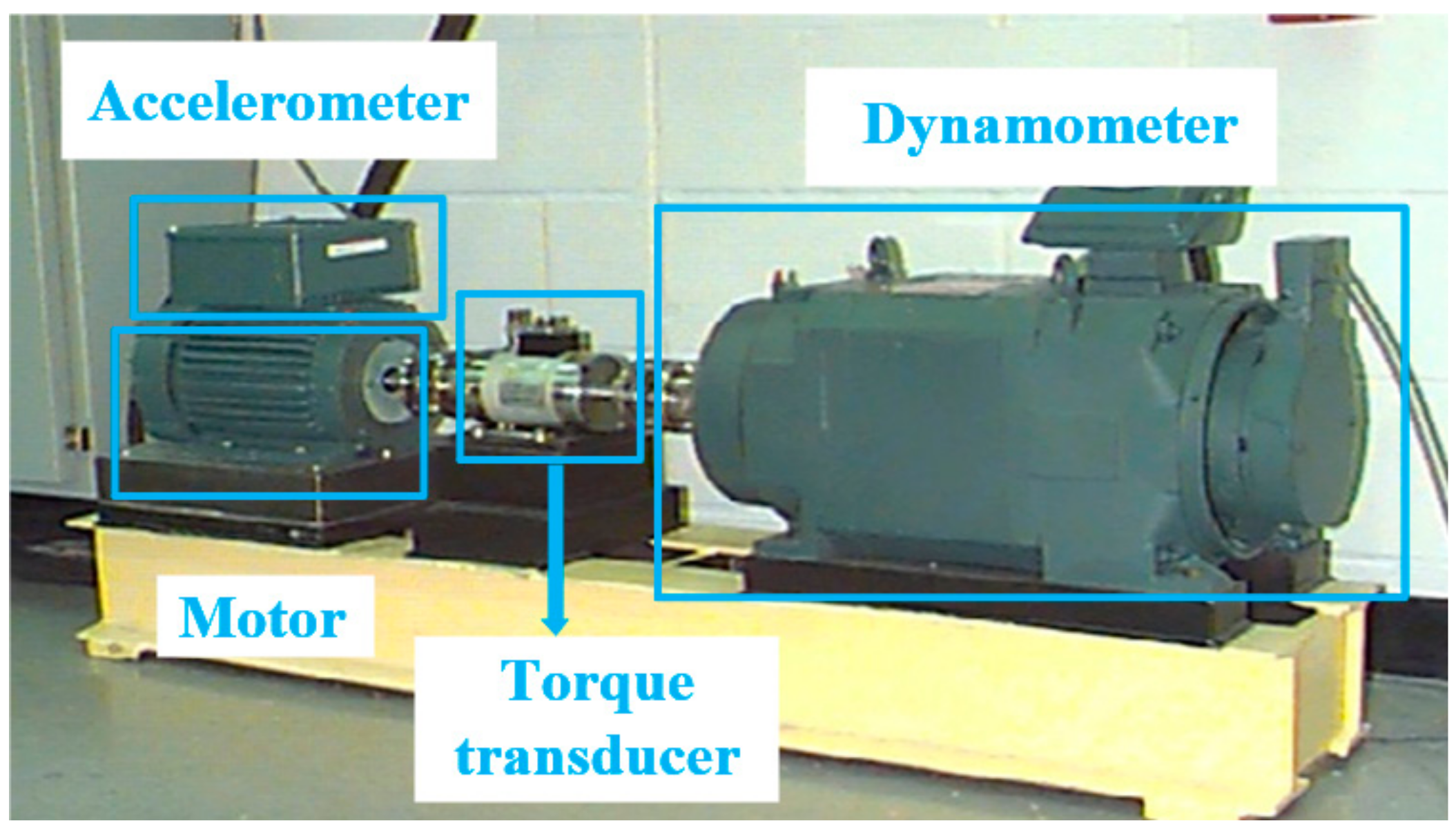
The primary experimental data used in this paper were gathered from the rolling bearing failure simulation platform at the CWRU Electrical Engineering Laboratory, which records vibration data from rolling bearings. As depicted in Figure 5, the test rig includes a two-horsepower motor, torque transducer, force gauge, and control electronics. The test bearing supports the motor shaft. For the experiments, the authors chose four different states as categories: normal, inner ring failure, outer ring failure, and ball failure. The raw dataset was divided in the following way: the fault data were categorized according to the normal state, the drive end at 12 kHz, the 48 kHz sampling frequency, and the fan end at 12 kHz sampling frequency, respectively. Each category contains inner ring, outer ring, and ball failure data at different failure depths and different horsepowers.

In order to meet the needs of fault diagnosis of portal crane drive motors under different working conditions and to comply with the requirements of the BRDATL network, we set four kinds of portal crane drive motors with different horsepower (ML0, ML1, ML2, and ML3) as the source domain and target domain data, respectively. The specific settings are as follows: ML0 is set as D1, ML1 is set as D2, ML2 is set as D3, and ML3 is set as D4. The detailed details of each horsepower data point are shown in

Table 1. Bearing Data Set Settings of CWRU.

Label	Health Condition	Source Domain	Training Target Domain	Test Target Domain
Nor	Normal	1000	500	500
I07	0.007 inner	100	50	50
O07	0.007 outer	100	50	50
B07	0.007 ball	100	50	50
I14	0.014 inner	100	50	50
O14	0.014 outer	100	50	50
B14	0.014 ball	100	50	50
I21	0.021 inner	100	50	50
O21	0.021 outer	100	50	50
B21	0.021 ball	100	50	50

. We set the ratio of data samples between the normal state and each fault state to 10:1, and every sample has 2560 data points. Through this setting, we can obtain representative data in the adversarial migration experiment of domain adaptation to each domain and help with the fault diagnosis research of the door drive motor.

(2)

XJTU-SY bearing dataset

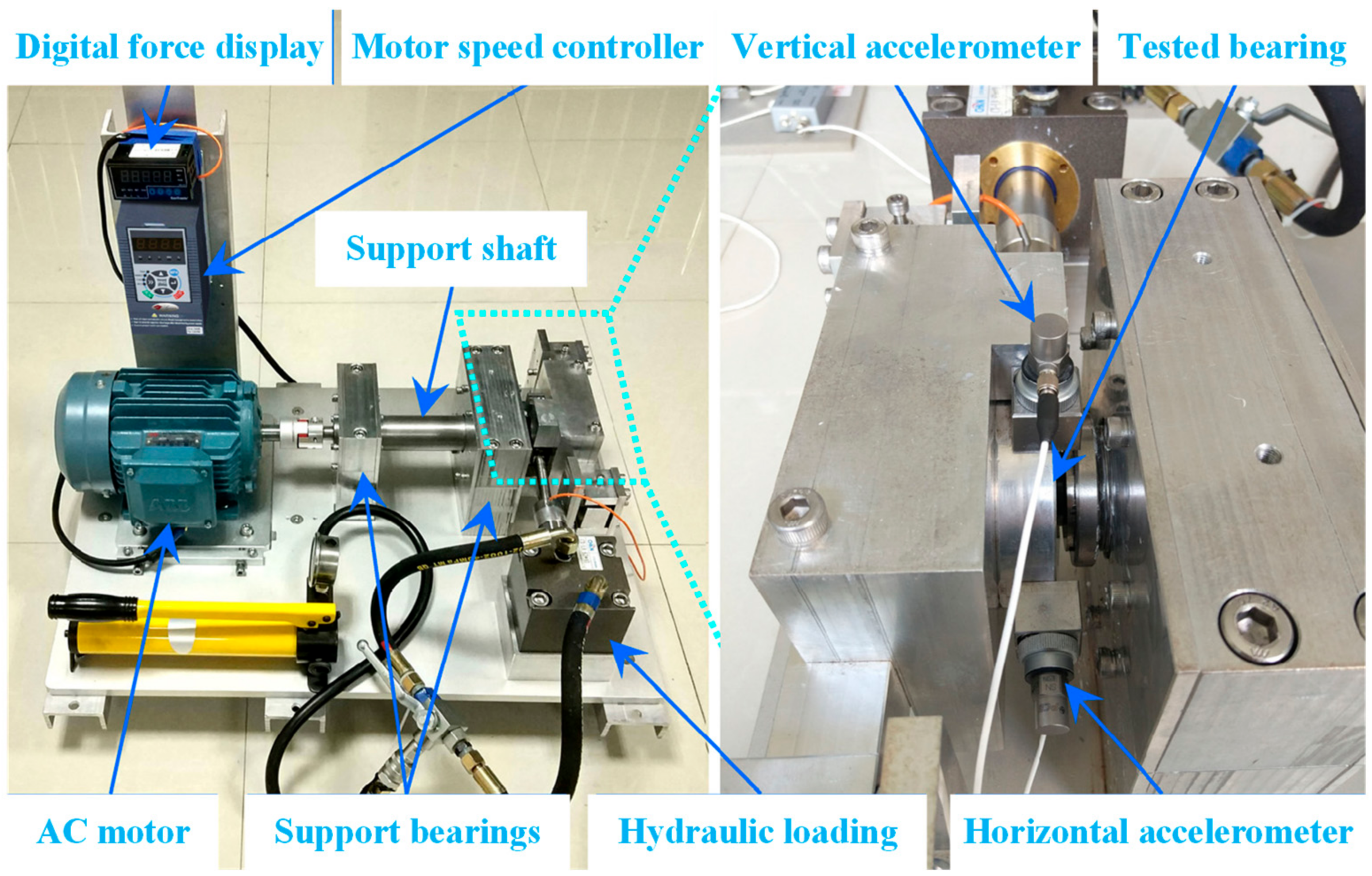
Considering that the CWRU bearing data set is the fault data obtained in the ideal environment, when verifying the BRDATL model proposed in this paper, there will be some limitations if only the CWRU data set is used. Therefore, this paper considers using the XJTU-SY bearing data set for further experimental verification. The XJTU-SY dataset contains the complete operation-to-failure data of 15 rolling bearings, which were obtained through many accelerated degradation experiments. The experimental platform is shown in Figure 6. A total of three working conditions were designed in the test, and there were five bearings under each condition.

Therefore, in order to meet the experimental requirements, this paper divides the data set into D5, D6, and D7 according to the working conditions. The detailed data for each working condition is shown in

Table 2. Bearing Data Set Settings of XJTU-SY.

Label	Health Condition	Source Domain	Training Target Domain	Test Target Domain
Nor	normal	500	300	300
IR	inner race	50	30	30
OR	outer race	50	30	30
CF	cage fault	50	30	30

, which includes the fault data at 2100 rpm, 2250 rpm, and 2400 rpm, respectively. Among them, each sample has 2048 data points.

5.3. Experimental Setup

The BRDATL network in this paper consists of a feature extractor, a label predictor, and a domain classifier with the structure shown in

Table 3. Network Architecture Components.

Input$x$
Feature Extractor${\Phi }_f$
GRU(forward)
GRU(reversed)
Dense	Flatten, Full Connected, Sigmoid, Dropout
Features$f(x)$
Label Predictor${\Phi }_l$		Domain Classifier${\Phi }_d$
Dense	Flatten, Full Connected Softmax	Dense	(ReLu, Dropout)*2 Flatten
		Dense	Full Connected, ReLu Full Connected, Softmax
Class		Domain

.

5.4. Comparative Experimental Analysis

To validate the superiority of the proposed BRDATL, other deep learning methods based on transfer learning are utilized for experimental comparison. All the other methods are composed of a feature extractor and a label predictor, as follows:

(1)

DAN: a base model where a multi-kernel variant (MK-MMD) of Maximum Mean Difference (MMD) is embedded into two fully connected layers (FC) for learning domain-invariant features.

(2)

DANN: a base model that enables adversarial domain classifiers to learn differential classifiers in the target domain.

(3)

DaNN: a dual-layer artificial neural network with an embedded MMD to match the source and target domains.

(4)

Deep Convolutional Adversarial Learning Networks (DCTLN) [38]: a base model where diagnostic knowledge is delivered by MMD using a domain classifier and domain adaptation module.

(5)

Domain Adversarial Transfer Network (DATN) [39]: a base model for domain adaptation using supervised training of task pairs for extraction and adversarial training of specific features.

(6)

Unsupervised Deep Transfer Learning (UDTL) [40]: a base model for feature learning and fault diagnosis based on unsupervised training on unbalanced datasets.

(7)

Deep Convolutional Domain Adversarial Transfer Learning (DCDATL) [41]: A new deep convolutional residual feature extractor is constructed to extract high-level features and improve the model accuracy after feature transfer.

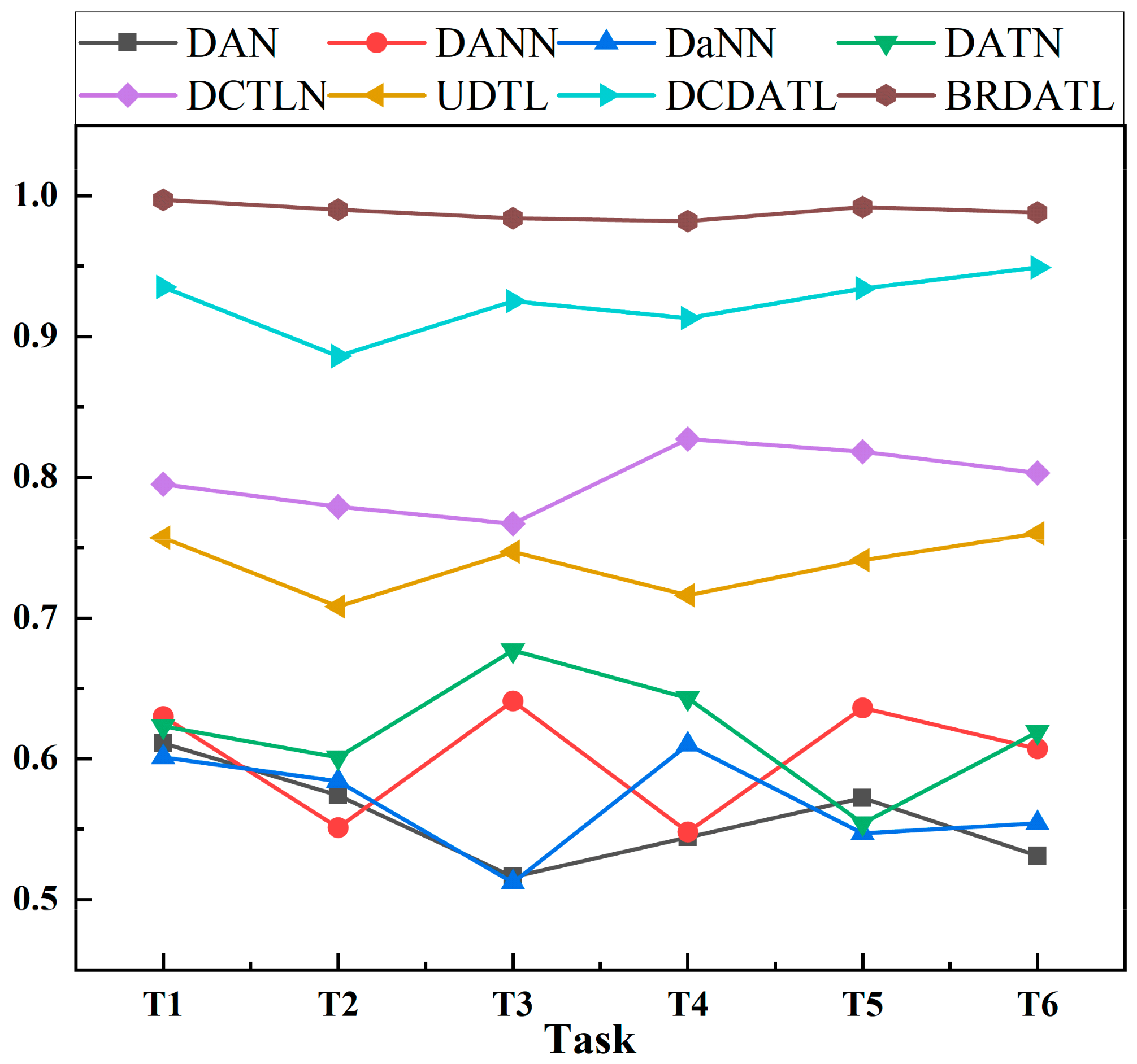
In order to reflect the performance of the model proposed in this paper in the inter-domain migration, the four data sets D1, D2, D3, and D4 were set as the source domain and the target domain for experiments to verify the accuracy of each model on the data set. In the command, D1-D2 indicates that D1 is used as the source domain, D2 is used as the target domain, and so on. The accuracy of all models in each experiment is shown in

Table 4. Diagnostic accuracy of different methods based on the CWRU bearing dataset.

Experment	DAN	DANN	DaNN	DATN	DCTLN	UDTL	DCDATL	BRDATL
D1-D2	0.526	0.526	0.536	0.538	0.78	0.761	0.897	0.994
D1-D3	0.526	0.526	0.526	0. 526	0.692	0.773	0.901	0.981
D1-D4	0.526	0.526	0.526	0.526	0.735	0.741	0.874	0.972
D2-D1	0.526	0.526	0.526	0.526	0.734	0.786	0.853	0.988
D2-D3	0.526	0.526	0.643	0.613	0.673	0.699	0.861	0.990
D2-D4	0.526	0.526	0.606	0.552	0.824	0.696	0.880	0.984
D3-D1	0.526	0.526	0.561	0.613	0.756	0.821	0.845	0.977
D3-D2	0.526	0.526	0.526	0.526	0.773	0.775	0.910	0.964
D3-D4	0.526	0.526	0.526	0.526	0.812	0.694	0.869	0.988
D4-D1	0.526	0.526	0.526	0.526	0.757	0.796	0.872	0.984
D4-D2	0.526	0.526	0.526	0.526	0.794	0.745	0.885	0.971
D4-D3	0.526	0.526	0.526	0.598	0.781	0.697	0.891	0.992

and Figure 7.

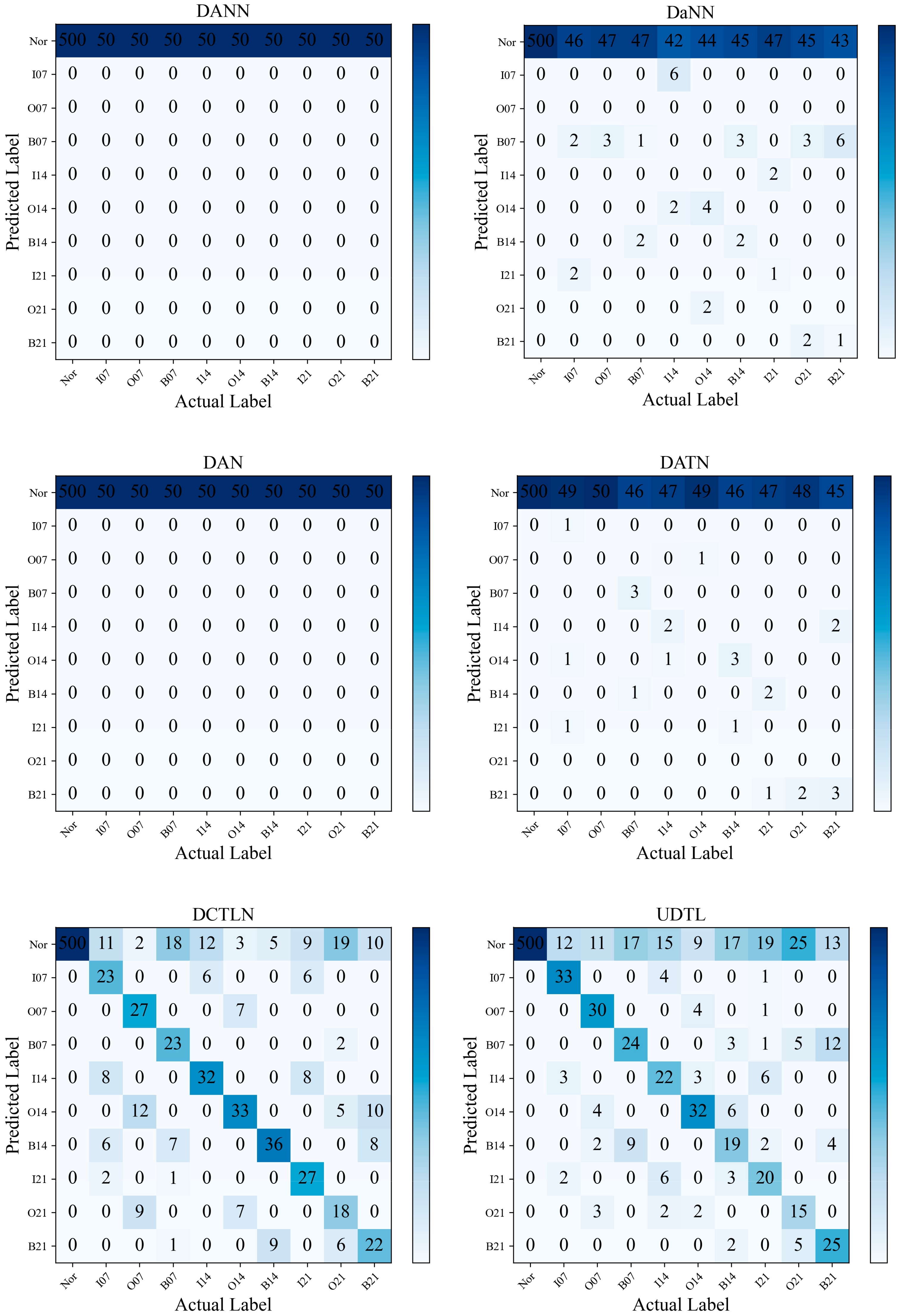
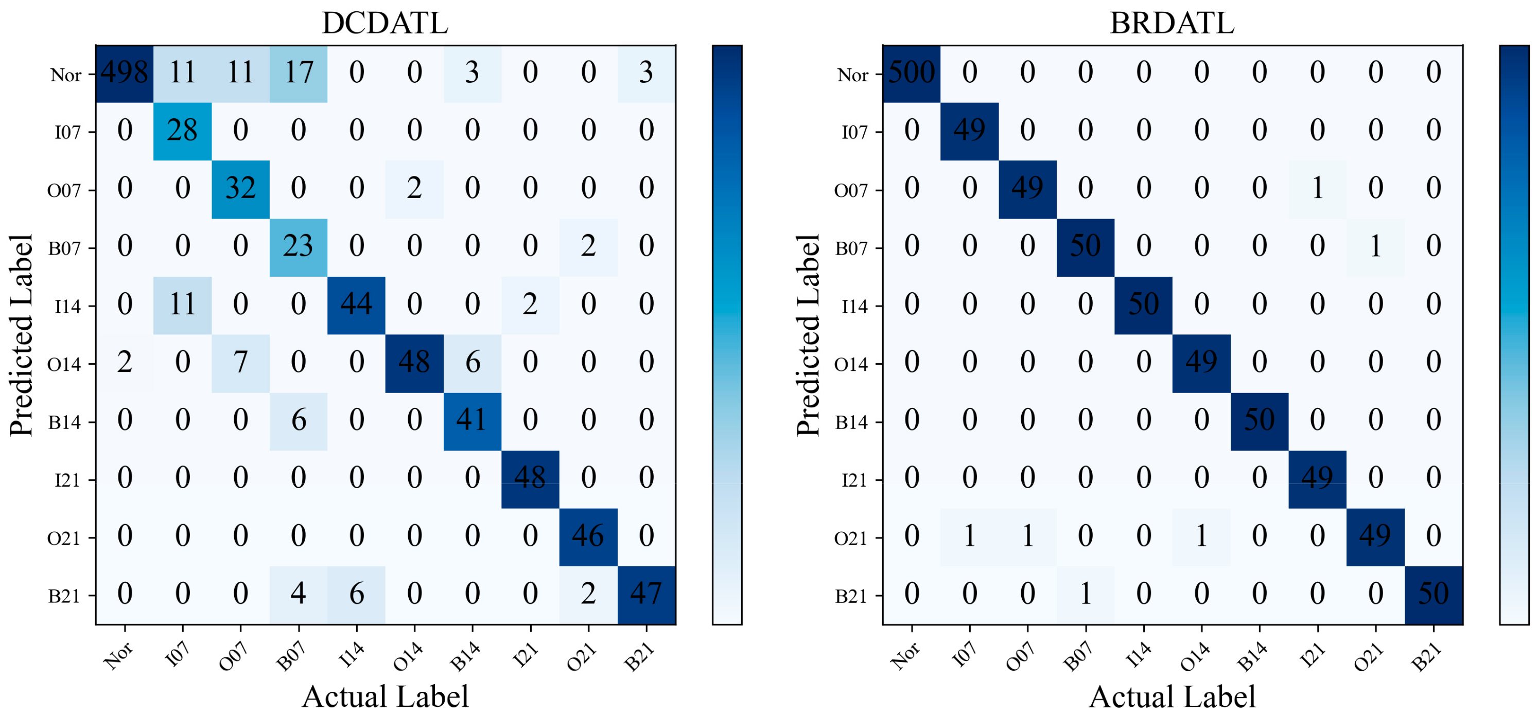
When D1 is the source domain and D2 is the target domain for the experiment based on the CWRU bearing dataset, the prediction accuracy of each model is shown in the confusion matrix in Figure 8. It can be seen that on DAN, DANN, DATN, and DaNN, almost all faults are recognized as normal states, which may be due to the “labeling bias” of the training data caused by the data imbalance, which results in the decision boundary of the labeled classifier not traversing the feature space of the secondary classes. UDTL and DATLN have better recognition accuracy than the above four methods, but their performance could be better for fault diagnosis. Whereas DCDATL has better recognition in the latter six classes, it has poor recognition with a fault depth of 0.007, whereas the BRDATL proposed in this paper recognizes almost all faults correctly.

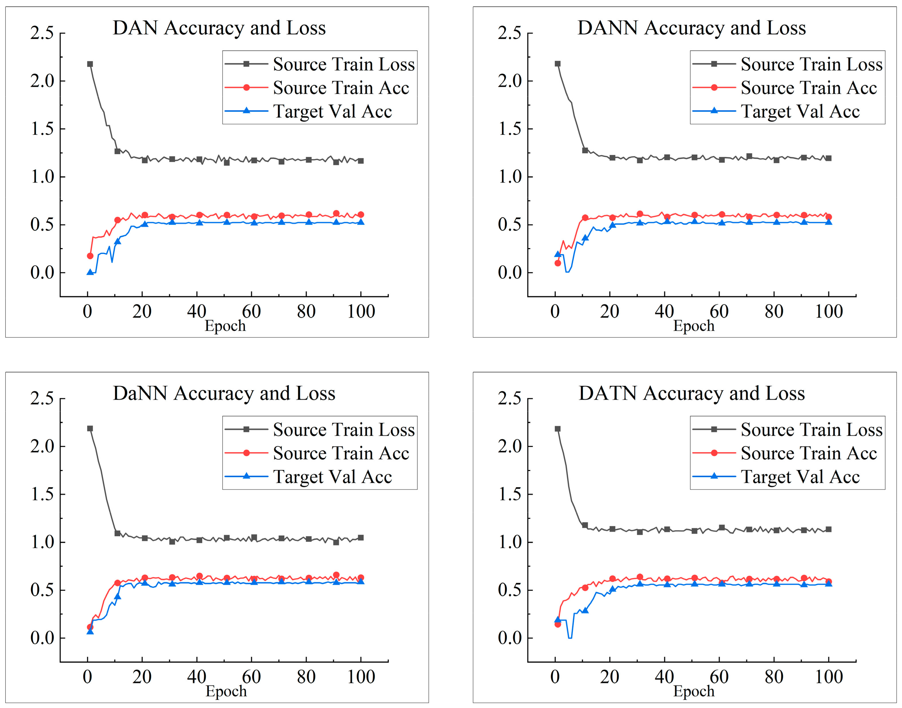
Figure 9 illustrates the training loss, training accuracy, and validation accuracy iterations of each model on tasks D1-D2. The four models DAN, DANN, DaNN, and DATN fluctuate a lot during training, and the training loss stays above 1, and the training accuracy and validation accuracy are around 50%. For the remaining four models, the models almost reach a stable convergence state when trained about 20 times, and the model validation accuracy of BRDATL can reach 99%. At the same time, as the model converges, the loss function begins to converge to 0. From the demonstrated results in Figure 8, it can be seen that although the three models UDTL, DATLN, and DCDATL have some diagnostic effect in the case of data imbalance, there is still a particular gap compared to the BRDATL proposed in this paper, which has a positive performance in data imbalance fault diagnosis.

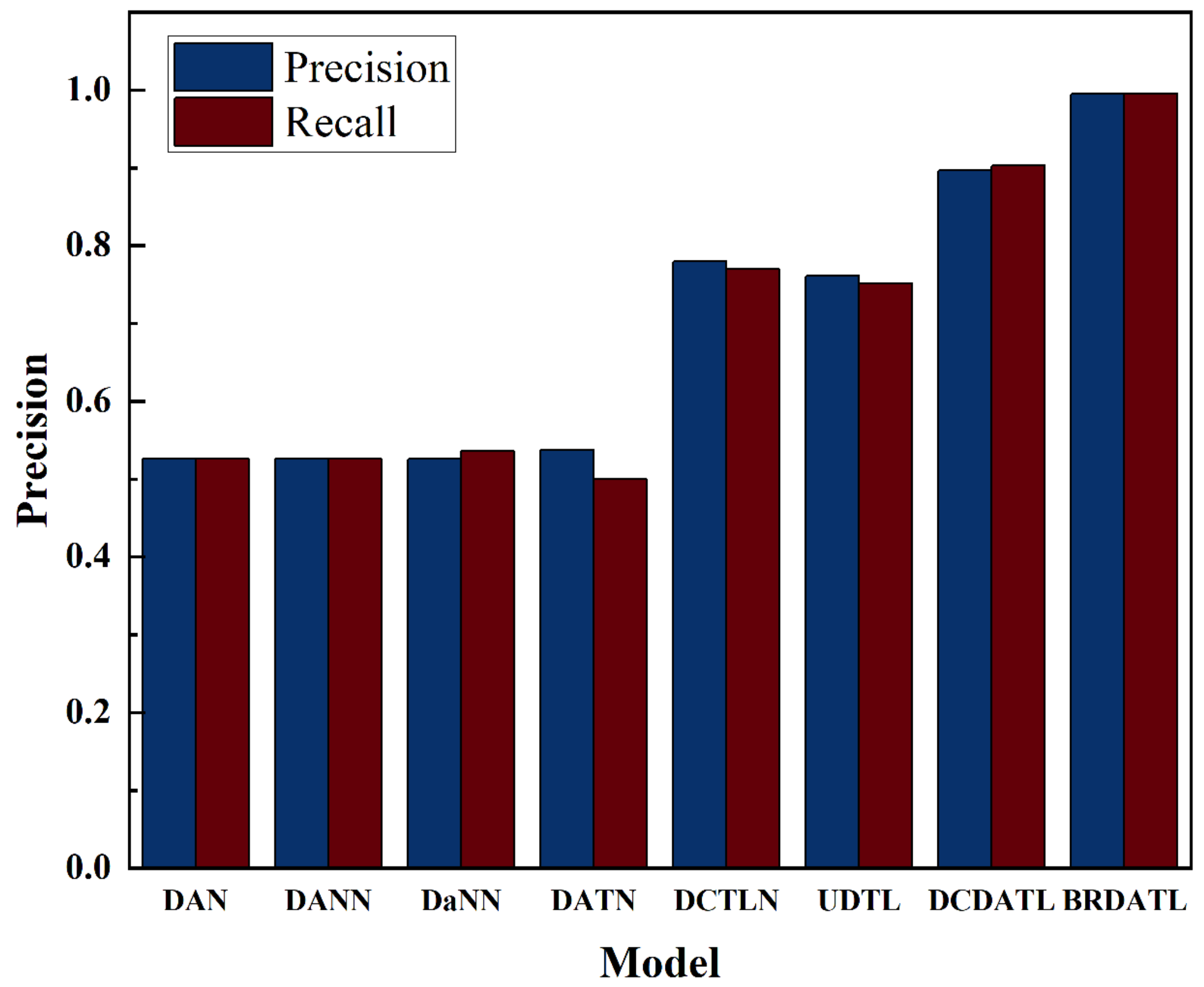
To further assess and compare the performance of each model, precision, recall, and F1 scores on each class are also used to analyze the performance of the models on the dataset set in this paper. They are defined as follows:

$$Precision=\frac{TrueP}{(TrueP+FauseP)}$$

(22)

$$Recall=\frac{TrueP}{(TrueP+FauseN)}$$

(23)

$$F_1-score=\frac{2\times TrueP}{(2TrueP+FauseP+FauseN)}$$

(24)

where $TrueP$ denotes the count of samples accurately classified as positive samples, $FauseP$ denotes the number of the count of samples inaccurately classified as positive samples, and $FauseN$ denotes the count of samples inaccurately classified as negative samples.

As shown in

Table 5. Precision, Recall, and F1 score of each model in each class.

Model	Precision	Recall	F1 Score
			Nor	I07	O07	B07	I15	O15	B15	I21	O21	B21
DAN	0.526	0.526	0.690	0	0	0	0	0	0	0	0	0
DANN	0.526	0.526	0.690	0	0	0	0	0	0	0	0	0
DaNN	0.526	0.536	0.711	0	0	0.029	0	0.153	0.075	0.038	0	0.038
DATN	0.538	0.50	0.701	0.038	0	0.152	0.073	0	0	0	0.039	0.109
DCTLN	0.78	0.77	0.918	0.551	0.653	0.613	0.653	0.6	0.673	0.675	0.529	0.5
UDTL	0.761	0.752	0.878	0.756	0.706	0.552	0.525	0.696	0.522	0.595	0.515	0.691
DCDATL	0.897	0.903	0.959	0.735	0.761	0.613	0.822	0.821	0.855	0.950	0.920	0.862
BRDATL	0.995	0.995	1	0.990	0.98	0.98	1	0.99	1	0.99	0.96	0.99

and Figure 10, DAN and DANN perform poorly in the F1 score due to the imbalance between the number of samples of different categories in the training dataset, i.e., the number of samples of the normal state is much greater than that of the other categories, thus leading to a poor F1 score, and DaNN and DATN perform poorly even though they recognize some of the states of some of the categories. The three parameters show that DCTLN and UDTL perform poorly on the F1 score, although both are above 75% in precision and recall. Moreover, although DCDATL performs superiorly to the above six models in the three evaluation indexes, there is still a gap with the BRDATL proposed in this paper.

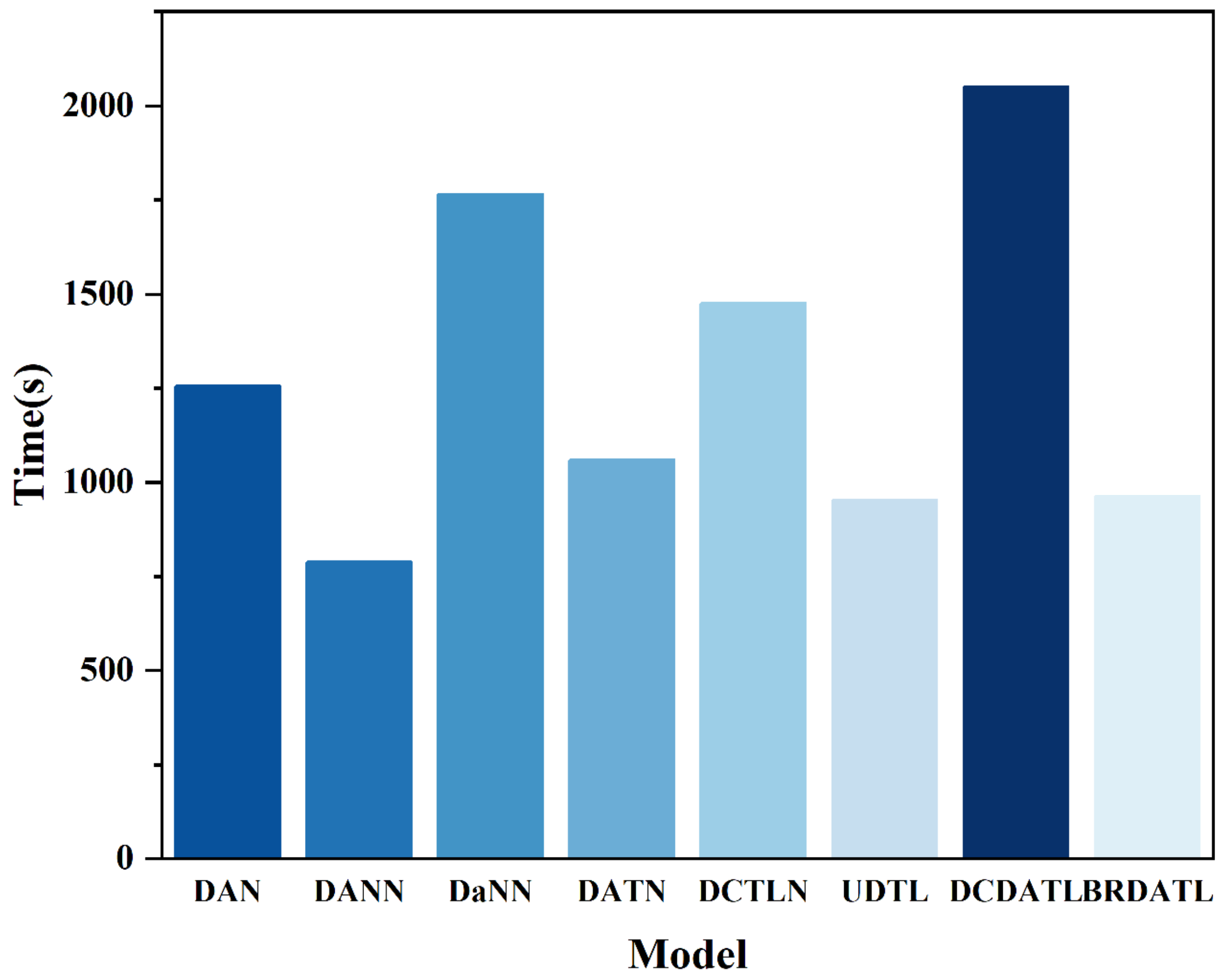
The training elapsed time as well as the core structure of the BRDATL proposed in this paper and other comparative experiments are shown in

Table 6. Training time for each model.

Model	Time (s)	Recall
DAN	1257	MK-MDD
DANN	789	Domain adversarial + GRL
DaNN	1765	MMD + Two-layer network
DATN	1061	Domain adversarial + Supervised training
DCTLN	1477	Multiple domain adaptation
UDTL	952	Domain adversarial + Unsupervised training
DCDATL	2051	Deep CNN + Domain adversarial
BRDATL	963	Bi-GRU + Domain adversarial

and Figure 11. It can be seen that although the BRDATL has positive results in terms of diagnostic accuracy, the training elapsed time is only the third least achieved due to the incorporation of the Bi-GRU for feature extraction.

5.5. Ablation Experiments

This section performs ablation experiments on the BRDATL model mentioned in this paper. The BRDATL model contains a feature extractor, label predictor, domain classifier, and loss optimization modules. The role of the ablation experiment is to remove some modules from the model to verify the effect of these modules on the model. We chose to remove the feature extractor, domain classifier, and loss optimization modules, respectively, to evaluate the effect of these modules on the performance of the model. In addition, this time, we choose to experiment on the D1-D3 task, and all other parameters remain unchanged when experimenting.

(1)

Remove-EF: Remove the feature extractor. The function of the feature extractor is to extract the features of the source and target domains, and it achieves feature alignment between these domains by considering the disparity between the feature distributions. It allows for observing the model’s troubleshooting ability on the source and target domain samples.

(2)

Remove-DC: Remove Domain Classifier. A domain classifier is used to distinguish between source and target domain features and then optimize the feature extractor to learn domain-invariant features by backpropagation. It allows for observing the model’s ability to handle domain differences.

(3)

Remove-LO: Remove the loss optimization module, which is used to automatically optimize each module’s loss function to better constrain the feature representation between the source and target domains. Try to remove the loss optimization module to observe the performance of the original model.

The results of the ablation experiments are shown in Figure 12. All the models were repeated 10 times, respectively, and the average accuracy domain mean square error of each module is shown in

Table 7. Average Accuracy and Mean Square Error of the Four Methods.

	Remove-EF	Remove-DC	Remove-LO	BRDATL
Average Accuracy	15.92%	53.61%	81.78%	98.51%
Mean Squared Error	72.59%	21.9%	3.51%	0.03%

and Figure 13. From the results, it can be seen that, compared to BRDATL, the removal of the other three modules results in a significant degradation of the model’s performance. Remove-EF and Remove-DC exhibit catastrophic performance, especially with diagnostic accuracies dropping to 15.92% and 53.61% and mean-square errors of 72.59% and 21.9%, respectively, where the mean square error quantifies the divergence between the observed and actual values; hence, a smaller value is preferable. Moreover, although Remove-LO performs well in accuracy, it cannot meet the needs of fault diagnosis. From the above, experimental removal of the feature extractor causes the model to be completely unable to learn effective feature representations, which leads to drastic performance degradation.

Hence, the role of Bi-GRU in the feature extraction of the whole model is very critical. Visual analysis can show that the learned feature representations of the model become chaotic, and it can be seen that in the ablation experiments, the features become indistinguishable after removing the feature extractor. Removing the domain classifier causes the feature extractor to lose the constraints of adversarial training, and the feature representations cannot be effectively aligned between the source and target domains, which reduces the domain adaptation performance of the model. Removing the loss optimization module causes the feature representations to be unconstrained between the source and target domains. The domain differences in the feature representations cannot be effectively reduced, thus affecting the domain adaptation performance of the model. Each module plays a vital role in domain adaptation training, and their combination enables the model to accomplish feature alignment between the source and target domains with positive domain adaptation performance.

5.6. Contrast Experiment

Based on the above experiments based on the CWRU bearing data set, in order to further verify the accuracy of the BRDATL model proposed in this paper, this section will conduct experiments on the modified XJTU-SY data set. After completing all the experiments, the results are shown in

Table 8. The diagnostic accuracy of different methods in this experiment is based on the XJTU-SY bearing dataset.

Task	Target Fault	Exprement	DAN	DANN	DaNN	DATN	DCTLN	UDTL	DCDATL	BRDATL
T1	OR,CF	D5-D6	0.611	0.630	0.601	0.623	0.795	0.757	0.935	0.997
T2	OR	D5-D7	0.574	0.551	0.584	0.601	0.779	0.708	0.886	0.990
T3	OR,CF	D6-D5	0.516	0.641	0.512	0.677	0.767	0.747	0.925	0.984
T4	IR,OR	D6-D7	0.544	0.548	0.610	0.643	0.827	0.716	0.913	0.982
T5	OR	D7-D5	0.572	0.636	0.547	0.554	0.818	0.741	0.934	0.992
T6	IR,OR	D7-D6	0.531	0.607	0.554	0.619	0.803	0.760	0.949	0.988

and Figure 14. Because D5 lacks inner ring fault data and D7 lacks cage fault data, the target faults identified by each task are different.

In addition, the t-SNE method can effectively map the high-order feature dimension to the low-order feature dimension to realize the visualization of features. Therefore, the performance of the BRDATL model on this data set can be clearly observed through the t-SNE diagram. As shown in Figure 15, it can be clearly seen that when BRDATL is tested in 6 tasks, in T1 and T3 tasks, due to the lack of inner ring fault data in D5, the recognition of inner ring fault samples is abnormal. In T4 and T6 tasks, due to the lack of cage fault data in D7, the cage fault identification is wrong. Finally, in the T2 and T5 tasks, due to the lack of samples of D5 and D7, the cage fault and inner ring fault are identified as abnormal. However, in the case of complete data, the boundary of the t-SNE diagram is obvious, and the type of fault can be well judged.

6. Conclusions

In this paper, a fault diagnosis method (BRDATL) based on transfer learning is proposed to solve the problem of unbalanced bearing samples of door drive motors. Based on the deep feature extraction capability of Bi-GRU in historical information, this paper proposes to use this network as a feature extractor against transfer learning to improve it. In order to improve the adaptive ability of the model and solve the problem of distribution differences between different domains under different working conditions, a new correlation maximum mean difference (CAMMD) is proposed to measure the distribution differences between domains. To verify the fault diagnosis performance of the model under the special working conditions of the door engine, the CWRU and XJTU-SY public datasets are first reclassified by different horsepower. Then, the samples of normal and fault states are set to 10:1 for simulation experiments and compared with the other seven models that have been proposed. The diagnostic accuracy of BRDATL in D1-D2 tasks is 99.4%, and the overall diagnostic accuracy is above 96.4%. In addition, BRDATL has precision and recall of 99.5%. In comparison experiments based on the XJTU-SY public data set, the accuracy of all diagnostic tasks was above 98.2%, and that of the T1 task reached 99.7%, which was significantly higher than other methods. The final experimental results show that the inclusion of Bi-GRU and the two unsupervised alignment methods are the reasons for the better performance of BRDATL compared to the other models, with better stability and accuracy in cross-domain diagnostic tasks with sample imbalance. This helps to solve the problem of “labeling bias” in the training data caused by the imbalance between the number of standard state samples and the number of fault samples and provides a feasible theoretical basis for the next step of bearing fault diagnosis of portal crane drive motors in natural industrial environments.

However, simulation experiments with unbalanced samples of faulty portal crane drive motor bearings were conducted only on labeled publicly available datasets, and the data generated from portal crane drive motors in natural industrial environments are characterized by instability and the absence of fault labels. The method proposed in this paper may have some limitations in fault diagnosis of unlabeled data, and there is a lack of similar data for comparison experiments. Future research is still needed to explore the possibility of implementing semi-supervised transfer learning in cross-domain fault diagnosis with insufficiently labeled and unbalanced source data. The problem of domain adaptation with data imbalance between different machines also needs to be addressed in real industrial scenarios to improve the accuracy and reliability of fault diagnosis. This will help to improve the diagnostic accuracy and liability for motor bearing faults, which are essential in real industrial applications, and promote the development of critical areas such as fault prediction and preventive maintenance.

References

- Wen, P.; Zhao, S.; Chen, S.; Li, Y. A Generalized Remaining Useful Life Prediction Method for Complex Systems Based on Composite Health Indicator. Reliab. Eng. Syst. Saf. 2021, 205, 107241. [Google Scholar] [CrossRef]
- Liu, R.; Yang, B.; Zio, E.; Chen, X. Artificial Intelligence for Fault Diagnosis of Rotating Machinery: A Review. Mech. Syst. Signal Process. 2018, 108, 33–47. [Google Scholar] [CrossRef]
- Lei, Y.; Yang, B.; Jiang, X.; Jia, F.; Li, N.; Nandi, A.K. Applications of Machine Learning to Machine Fault Diagnosis: A Review and Roadmap. Mech. Syst. Signal Process. 2020, 138, 106587. [Google Scholar] [CrossRef]
- Li, X.; Zhang, W.; Ding, Q.; Li, X. Diagnosing Rotating Machines With Weakly Supervised Data Using Deep Transfer Learning. IEEE Trans. Ind. Inf. 2020, 16, 1688–1697. [Google Scholar] [CrossRef]
- Wu, H.; Ma, X.; Wen, C. Multilevel Fine Fault Diagnosis Method for Motors Based on Feature Extraction of Fractional Fourier Transform. Sensors 2022, 22, 1310. [Google Scholar] [CrossRef] [PubMed]
- Yan, X.; Liu, Y.; Jia, M. A Fault Diagnosis Approach for Rolling Bearing Integrated SGMD, IMSDE and Multiclass Relevance Vector Machine. Sensors 2020, 20, 4352. [Google Scholar] [CrossRef]
- You, W.; Shen, C.; Guo, X.; Jiang, X.; Shi, J.; Zhu, Z. A Hybrid Technique Based on Convolutional Neural Network and Support Vector Regression for Intelligent Diagnosis of Rotating Machinery. Adv. Mech. Eng. 2017, 9, 168781401770414. [Google Scholar] [CrossRef]
- Ren, L.; Sun, Y.; Cui, J.; Zhang, L. Bearing Remaining Useful Life Prediction Based on Deep Autoencoder and Deep Neural Networks. J. Manuf. Syst. 2018, 48, 71–77. [Google Scholar] [CrossRef]
- Zhou, J.; Xiao, M.; Niu, Y.; Ji, G. Rolling Bearing Fault Diagnosis Based on WGWOA-VMD-SVM. Sensors 2022, 22, 6281. [Google Scholar] [CrossRef]
- Wang, L.; Liu, Z. An Improved Local Characteristic-Scale Decomposition to Restrict End Effects, Mode Mixing and Its Application to Extract Incipient Bearing Fault Signal. Mech. Syst. Signal Process. 2021, 156, 107657. [Google Scholar] [CrossRef]
- Li, Y.; Song, L.; Sun, Q.; Xu, H.; Li, X.; Fang, Z.; Yao, W. Rolling Bearing Fault Diagnosis Based on Quantum LS-SVM. EPJ Quantum Technol. 2022, 9, 18. [Google Scholar] [CrossRef]
- Zhiwei, L. Bearing Fault Diagnosis of End-to-End Model Design Based on 1DCNN-GRU Network. Discret. Dyn. Nat. Soc. 2022, 2022, 7167821. [Google Scholar] [CrossRef]
- Chen, H.; Meng, W.; Li, Y.; Xiong, Q. An Anti-Noise Fault Diagnosis Approach for Rolling Bearings Based on Multiscale CNN-LSTM and a Deep Residual Learning Model. Meas. Sci. Technol. 2023, 34, 045013. [Google Scholar] [CrossRef]
- Kumar, A.; Parey, A.; Kankar, P.K. A New Hybrid LSTM-GRU Model for Fault Diagnosis of Polymer Gears Using Vibration Signals. J. Vib. Eng. Technol. 2023, 1–13. [Google Scholar] [CrossRef]
- Guo, Y.; Mao, J.; Zhao, M. Rolling Bearing Fault Diagnosis Method Based on Attention CNN and BiLSTM Network. Neural Process. Lett. 2023, 55, 3377–3410. [Google Scholar] [CrossRef]
- Ghifary, M.; Kleijn, W.B.; Zhang, M. Domain Adaptive Neural Networks for Object Recognition. In Proceedings of the PRICAI 2014: Trends in Artificial Intelligence, Gold Coast, QLD, Australia, 1–5 December 2014; Pham, D.-N., Park, S.-B., Eds.; Springer International Publishing: Cham, Switzerland, 2014; pp. 898–904. [Google Scholar]
- Long, M.; Cao, Y.; Wang, J.; Jordan, M. Learning Transferable Features with Deep Adaptation Networks. In Proceedings of the 32nd International Conference on Machine Learning, Lille, France, 7–9 July 2015; Bach, F., Blei, D., Eds.; PMLR: Lille, France, 2015; Volume 37, pp. 97–105. [Google Scholar]
- Ganin, Y.; Lempitsky, V. Unsupervised Domain Adaptation by Backpropagation. In Proceedings of the 32nd International Conference on Machine Learning, Lille, France, 7–9 July 2015; Bach, F., Blei, D., Eds.; PMLR: Lille, France, 2015; Volume 37, pp. 1180–1189. [Google Scholar]
- Zhang, R.; Tao, H.; Wu, L.; Guan, Y. Transfer Learning With Neural Networks for Bearing Fault Diagnosis in Changing Working Conditions. IEEE Access 2017, 5, 14347–14357. [Google Scholar] [CrossRef]
- Chen, D.; Yang, S.; Zhou, F. Incipient Fault Diagnosis Based on DNN with Transfer Learning. In Proceedings of the 2018 International Conference on Control, Automation and Information Sciences (ICCAIS), Hangzhou, China, 24–27 October 2018; IEEE: Hangzhou, China, 2018; pp. 303–308. [Google Scholar]
- Li, X.; Hu, Y.; Zheng, J.; Li, M.; Ma, W. Central Moment Discrepancy Based Domain Adaptation for Intelligent Bearing Fault Diagnosis. Neurocomputing 2021, 429, 12–24. [Google Scholar] [CrossRef]
- Cheng, C.; Zhou, B.; Ma, G.; Wu, D.; Yuan, Y. Wasserstein Distance Based Deep Adversarial Transfer Learning for Intelligent Fault Diagnosis with Unlabeled or Insufficient Labeled Data. Neurocomputing 2020, 409, 35–45. [Google Scholar] [CrossRef]
- Zou, Y.; Liu, Y.; Deng, J.; Jiang, Y.; Zhang, W. A Novel Transfer Learning Method for Bearing Fault Diagnosis under Different Working Conditions. Measurement 2021, 171, 108767. [Google Scholar] [CrossRef]
- Tong, Z.; Li, W.; Zhang, B.; Jiang, F.; Zhou, G. Bearing Fault Diagnosis Under Variable Working Conditions Based on Domain Adaptation Using Feature Transfer Learning. IEEE Access 2018, 6, 76187–76197. [Google Scholar] [CrossRef]
- Zhao, K.; Jiang, H.; Wu, Z.; Lu, T. A Novel Transfer Learning Fault Diagnosis Method Based on Manifold Embedded Distribution Alignment with a Little Labeled Data. J. Intell. Manuf. 2022, 33, 151–165. [Google Scholar] [CrossRef]
- Wang, Z.; He, X.; Yang, B.; Li, N. Subdomain Adaptation Transfer Learning Network for Fault Diagnosis of Roller Bearings. IEEE Trans. Ind. Electron. 2022, 69, 8430–8439. [Google Scholar] [CrossRef]
- Zhang, A.; Gao, X. Supervised Dictionary-Based Transfer Subspace Learning and Applications for Fault Diagnosis of Sucker Rod Pumping Systems. Neurocomputing 2019, 338, 293–306. [Google Scholar] [CrossRef]
- Han, T.; Liu, C.; Wu, R.; Jiang, D. Deep Transfer Learning with Limited Data for Machinery Fault Diagnosis. Appl. Soft Comput. 2021, 103, 107150. [Google Scholar] [CrossRef]
- Dong, Y.; Li, Y.; Zheng, H.; Wang, R.; Xu, M. A New Dynamic Model and Transfer Learning Based Intelligent Fault Diagnosis Framework for Rolling Element Bearings Race Faults: Solving the Small Sample Problem. ISA Trans. 2022, 121, 327–348. [Google Scholar] [CrossRef]
- Ji, M.; Peng, G.; He, J.; Liu, S.; Chen, Z.; Li, S. A Two-Stage, Intelligent Bearing-Fault-Diagnosis Method Using Order-Tracking and a One-Dimensional Convolutional Neural Network with Variable Speeds. Sensors 2021, 21, 675. [Google Scholar] [CrossRef]
- Zuo, L.; Xu, F.; Zhang, C.; Xiahou, T.; Liu, Y. A Multi-Layer Spiking Neural Network-Based Approach to Bearing Fault Diagnosis. Reliab. Eng. Syst. Saf. 2022, 225, 108561. [Google Scholar] [CrossRef]
- Yu, H.; Wang, K.; Li, Y.; He, M. Deep Subclass Reconstruction Network for Fault Diagnosis of Rotating Machinery under Various Operating Conditions. Appl. Soft Comput. 2021, 112, 107755. [Google Scholar] [CrossRef]
- Ding, X.; Wang, H.; Cao, Z.; Liu, X.; Liu, Y.; Huang, Z. An Edge Intelligent Method for Bearing Fault Diagnosis Based on a Parameter Transplantation Convolutional Neural Network. Electronics 2023, 12, 1816. [Google Scholar] [CrossRef]
- Ma, X.; Si, Y.; Yuan, Z.; Qin, Y.; Wang, Y. Multistep Dynamic Slow Feature Analysis for Industrial Process Monitoring. IEEE Trans. Instrum. Meas. 2020, 69, 9535–9548. [Google Scholar] [CrossRef]
- Xu, Y.; Li, Z.; Wang, S.; Li, W.; Sarkodie-Gyan, T.; Feng, S. A Hybrid Deep-Learning Model for Fault Diagnosis of Rolling Bearings. Measurement 2021, 169, 108502. [Google Scholar] [CrossRef]
- Maurya, S.; Verma, N.K. Intelligent Hybrid Scheme for Health Monitoring of Degrading Rotary Machines: An Adaptive Fuzzy c -Means Coupled With 1-D CNN. IEEE Trans. Instrum. Meas. 2023, 72, 1–10. [Google Scholar] [CrossRef]
- Creswell, A.; White, T.; Dumoulin, V.; Arulkumaran, K.; Sengupta, B.; Bharath, A.A. Generative Adversarial Networks: An Overview. IEEE Signal Process. Mag. 2018, 35, 53–65. [Google Scholar] [CrossRef]
- Guo, L.; Lei, Y.; Xing, S.; Yan, T.; Li, N. Deep Convolutional Transfer Learning Network: A New Method for Intelligent Fault Diagnosis of Machines With Unlabeled Data. IEEE Trans. Ind. Electron. 2019, 66, 7316–7325. [Google Scholar] [CrossRef]
- Chen, Z.; He, G.; Li, J.; Liao, Y.; Gryllias, K.; Li, W. Domain Adversarial Transfer Network for Cross-Domain Fault Diagnosis of Rotary Machinery. IEEE Trans. Instrum. Meas. 2020, 69, 8702–8712. [Google Scholar] [CrossRef]
- Zhao, Z.; Zhang, Q.; Yu, X.; Sun, C.; Wang, S.; Yan, R.; Chen, X. Applications of Unsupervised Deep Transfer Learning to Intelligent Fault Diagnosis: A Survey and Comparative Study. IEEE Trans. Instrum. Meas. 2021, 70, 1–28. [Google Scholar] [CrossRef]
- Li, F.; Tang, T.; Tang, B.; He, Q. Deep Convolution Domain-Adversarial Transfer Learning for Fault Diagnosis of Rolling Bearings. Measurement 2021, 169, 108339. [Google Scholar] [CrossRef]
Figure 1.
Network framework of GRU.
Figure 2.
Diagram of the Bi-GRU structure.
Figure 3.
Diagram of the BRDATL.