Comparative Study on Coordinated Control of Path Tracking and Vehicle Stability for Autonomous Vehicles on Low-Friction Roads

Abstract

This paper presents a comparative study on coordinated control of path tracking and vehicle stability for autonomous vehicles on low-friction roads. Generally, a path-tracking controller designed on high-friction roads cannot provide good performance under low-friction conditions. To cope with the problem, a coordinated control between path tracking and vehicle stability has been proposed to date. In this paper, three types of coordinated controllers are classified according to the controller structure. As an actuator, front-wheel steering, four-wheel steering, and four-wheel independent braking and driving are adopted. A common feature of these types of controllers is that front steering and yaw moment control are adopted as control inputs. To convert the yaw moment control into tire forces generated by combinations of multiple actuators, a control allocation method is applied. For each type, a controller is designed and simulated using vehicle simulation software. From the simulation results, a performance comparison among those controller types is carried out. Through comparison, it is shown that there are small differences among those types of controllers in terms of path tracking.

1. Introduction

Autonomous driving has been regarded as a next-generation solution for future transportation in research groups and the automotive industry since 2010 because it can prevent several types of traffic accidents and make road safety and traffic flow better [1,2,3]. From the literature survey, it is widely known that a generic modular system architecture for autonomous driving comprises detection, localization, prediction, planning, and control [2]. Among those topics, path-tracking control (PTC) has been intensively studied [4,5]. Consequently, a great deal of papers have been published in the area of PTC [4,5,6,7,8,9,10].

The aim of PTC is to make a vehicle follow a target path. For this purpose, most of the path-tracking controllers proposed to date have tried to minimize the lateral offset error (e_y) and heading error (e_φ), which are derived from the current vehicle position and target path [8,9]. Generally, front-wheel steering (FWS) or four-wheel steering (4WS) has been adopted as a control input or an actuator of a path-tracking controller. In this paper, 4WS means the combination of FWS and rear-wheel steering (RWS). This controller has shown good performance for path tracking on high-friction roads because this is designed and tuned under high-friction conditions. However, a PTC designed on high-friction roads cannot provide good performance under low-friction conditions [11,12,13]. This is caused by the fact that the lateral tire force of a vehicle becomes small on low-friction roads. To cope with the problem, PTC has been integrated with vehicle stability or lateral stability control. Vehicle stability control (VSC) has been intensively studied since the middle of the 1990s [14,15,16,17]. In this paper, VSC stands for yaw rate tracking and lateral stability controls, where the former tries to minimize the yaw rate error (γ_e) and the latter tries to keep the side-slip angle (β) as small as possible. Generally, the yaw moment control (∆M_z) has been adopted as a control input of VSC. ∆M_z is a virtual input, which should be generated by multiple actuators installed in real vehicles. For this reason, ∆M_z is to be converted into the tire forces generated by multiple actuators. This procedure is called control allocation or yaw moment distribution. Actuators used to generate ∆M_z are FWS, 4WS, RWS, and four-wheel independent steering/driving/braking (4WIS/4WID/4WIB) [18,19]. Most control allocation methods are quadratic programming (QP) with equality or/and inequality constraints [11,12,13,18,19].

Numerous papers have been published on the coordinated control of path tracking and vehicle stability on low-friction road conditions [11,12,13,20,21,22,23,24,25,26,27,28,29,30,31,32,33,34,35,36,37,38,39,40]. These papers can be classified into three types. Figure 1 shows the control structures of these types.

The first type of coordinated control method is to use two-level controllers: upper- and lower-level controllers [13,20,21,22,23,24,25,26,27,28,29]. As a control input, steering angles and ∆M_z are calculated by controllers such as model predictive control (MPC), PID control, sliding mode control (SMC), and H_∞ control in the upper-level controllers (UPLC). Among the control inputs, steering angles and ∆M_z are in charge of PTC and VSC in low-friction roads, respectively. For controller design, most of these types of controllers adopted a state-space model with e_y, e_φ, and its rates. ∆M_z is converted into tire forces generated by a single actuator or a combination of multiple ones such as FWS, RWS, 4WS, 4WIS, 4WIB, and 4WID in the lower-level controller (LWLC). For this purpose, a control allocation method was adopted. The steering angles of FWS, RWS, and 4WS, and braking and traction torques of 4WID and 4WIB are calculated from the converted tire forces. The effects of combinations of multiple actuators on path-tracking performance were deeply investigated in the previous research [13]. According to this work, there are few differences among the combinations of FWS, 4WS, 4WID, and 4WIB in terms of path-tracking performance. In other words, it is quite enough to use only FWS for path tracking. Let us denote this type of method as PTC#1.

The second type of coordinated control method is to use three-level controllers: upper-, middle-, and lower-level controllers [12,30,31,32,33,34,35,36,37]. In the UPLC, the front steering angle is calculated by a driver model or a controller. As a driver model, pure pursuit and Stanley methods have been widely used to date [4,11,12]. As a controller for steering angle generation, linear quadratic regulator (LQR), MPC, and SMC have been widely adopted with the state-space model whose state variables are e_y and e_φ. This is identical to PTC#1 with FWS. In the middle-level controller (MDLC), a reference yaw rate (γ_ref) is calculated from the front steering angle (δ_f), and a controller is designed to calculate ∆M_z, which is needed to make a vehicle follow the reference yaw rate. Most of MDLCs adopted SMC in order to calculate ∆M_z. In the previous paper, the reference yaw rate is directly generated as a control input of the UPLC, H_∞ control [34]. In the LWLC, ∆M_z is converted into tire forces generated by multiple actuators. For this purpose, a control allocation method is applied. Let us denote this type of method as PTC#2. In view of PTC#1, it seems unnecessary to use the three-level controller of PTC#2 because PTC#1 has the upper- and middle-level controllers of PTC#2 in the UPLC. In other words, to generate ∆M_z, PTC#2 requires two controllers although PTC#1 does a single controller. If the path-tracking performance of PTC#2 is not superior to that of PTC#1 on low-friction roads, then PTC#2 is useless.

The third type of coordinated control method is identical to the second one except that the reference yaw rate is obtained from a target path in the UPLC [11,38,39,40]. In this type of method, a driver model or LQR is needed to generate δ_f. In the MDLC of this method, SMC has been applied to calculate ∆M_z, which is needed to make a vehicle follow the reference yaw rate. In the LWLC, a control allocation method was applied to convert ∆M_z into tire forces generated by multiple actuators such as RWS, 4WID, and 4WIB. Let us denote this type of method as PTC#3. In view of PTC#1, PTC#3 has the identical problem to PTC#2 because PTC#3 has a three-level structure.

The first feature of PTC#1, PTC#2, and PTC#3 is the control allocation in LWLC, which is applied to distribute ∆M_z into tire forces generated by combinations of multiple actuators. In fact, control allocation and LWLC are synonymous. For control allocation, an optimization method with QP has been applied to date. These are quite general in vehicle stability control or lateral stability control. For this reason, PTC#1, PTC#2, and PTC3 try to integrate path tracking and vehicle stability control for driving on low-friction roads.

The second feature of PTC#2 and PTC#3 is the calculation procedure of γ_ref. PTC#1 does not use γ_ref. In PTC#2 and PTC#3, γ_ref for path tracking is calculated from δ_f or a target path in the MDLC. In PTC#1, PTC#2, and PTC#3, δ_f is generated using LQR. Because δ_f is already determined using LQR in the UPLC, it is excluded from the control allocation procedure. In other words, δ_f is not determined using the control allocation procedure. For this reason, the actuators used for control allocation are RWS, 4WID, and 4WIB.

The third feature of these methods is to use a preview or lookahead function along the heading direction [12,21,22,24,34,38,40]. Generally, the larger the preview distance the smaller the steering angle. Especially, the preview distance should be larger for lateral stability on low-friction roads. On the contrary, the preview distance should be smaller for path tracking on high-friction roads [12,41]. For this reason, the preview distance should be carefully tuned for path tracking and lateral stability if it is adopted [13].

The aim of this paper is to compare three types of coordinated controllers, PTC#1, PTC#2, and PTC#3, for PTC and VSC on low-friction road conditions. As a state variable, e_y, e_φ, β, and γ are selected, and these variables are included in the LQ objective function for PTC and VSC. In the state-space model, a preview function is introduced. In PTC#1, four input configurations, [δ_f], [δ_f δ_r], [δ_f ∆M_z] and [δ_f δ_r ∆M_z], are selected from three control inputs, δ_f, δ_r, and ∆M_z. If ∆M_z is selected as a control input, a control allocation method is adopted to distribute it to the tire forces generated using multiple actuators. As an actuator for control allocation, 4WID and 4WIB are adopted [13,39]. To compare those controllers, a simulation is conducted using the vehicle simulation package, CarSim. The double lane change maneuver for collision avoidance is adopted as a test scenario [11,12,20,26,27,37]. From the simulation results, it is shown that there are few differences among the three types of coordinated controllers on low-friction roads.

The contributions of this paper can be condensed as follows:

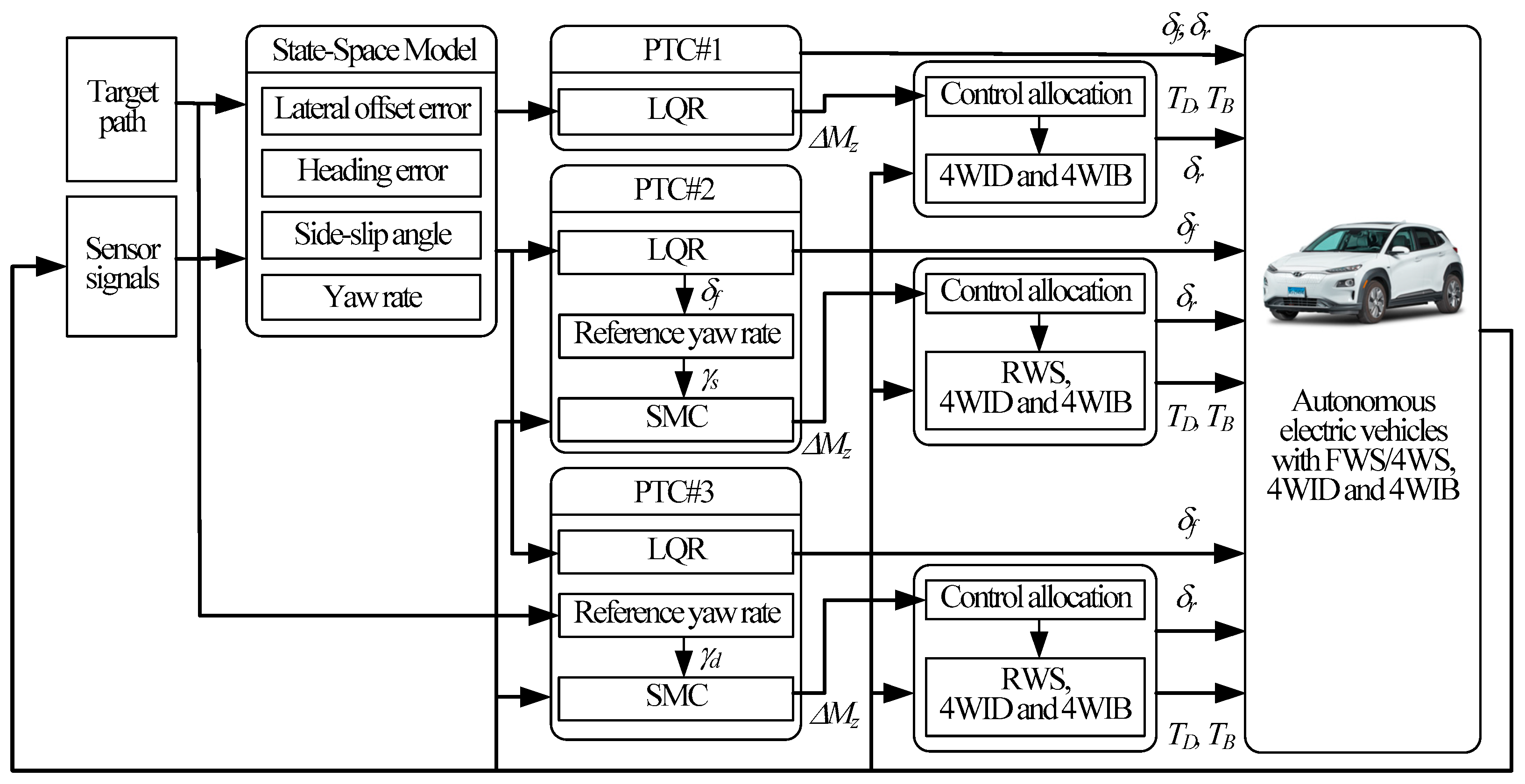
• This paper compares three types of coordinated controllers for PTC and VSC using LQR with regard to path-tracking performance. Different from the previous works, β and γ are included as state variables instead of the rates of lateral offset and heading errors. A preview function is also introduced into the state-space model. With the state vector, it is easier to include the preview function in the state-space model.
• Through comparison, the effects of input configurations and controller structures on path-tracking performance under low-friction conditions were investigated. With the investigation, which type of controller is more effective than others for path tracking is determined.
• From the comparison results, the best control structure and input configuration for path tracking and vehicle stability on low-friction roads is recommended. If there are little differences among those types of controllers, the simplest one is the best.

This paper consists of five sections. A design procedure of three types of coordinated controllers is described in Section 2. In Section 3, several measures for path-tracking performance are presented. The simulation is carried out and the simulation results are discussed in terms of the performance measures in Section 4. The conclusion is provided in Section 5.

2. Design of Controllers for Coordinated Control of Path Tracking and Vehicle Stability

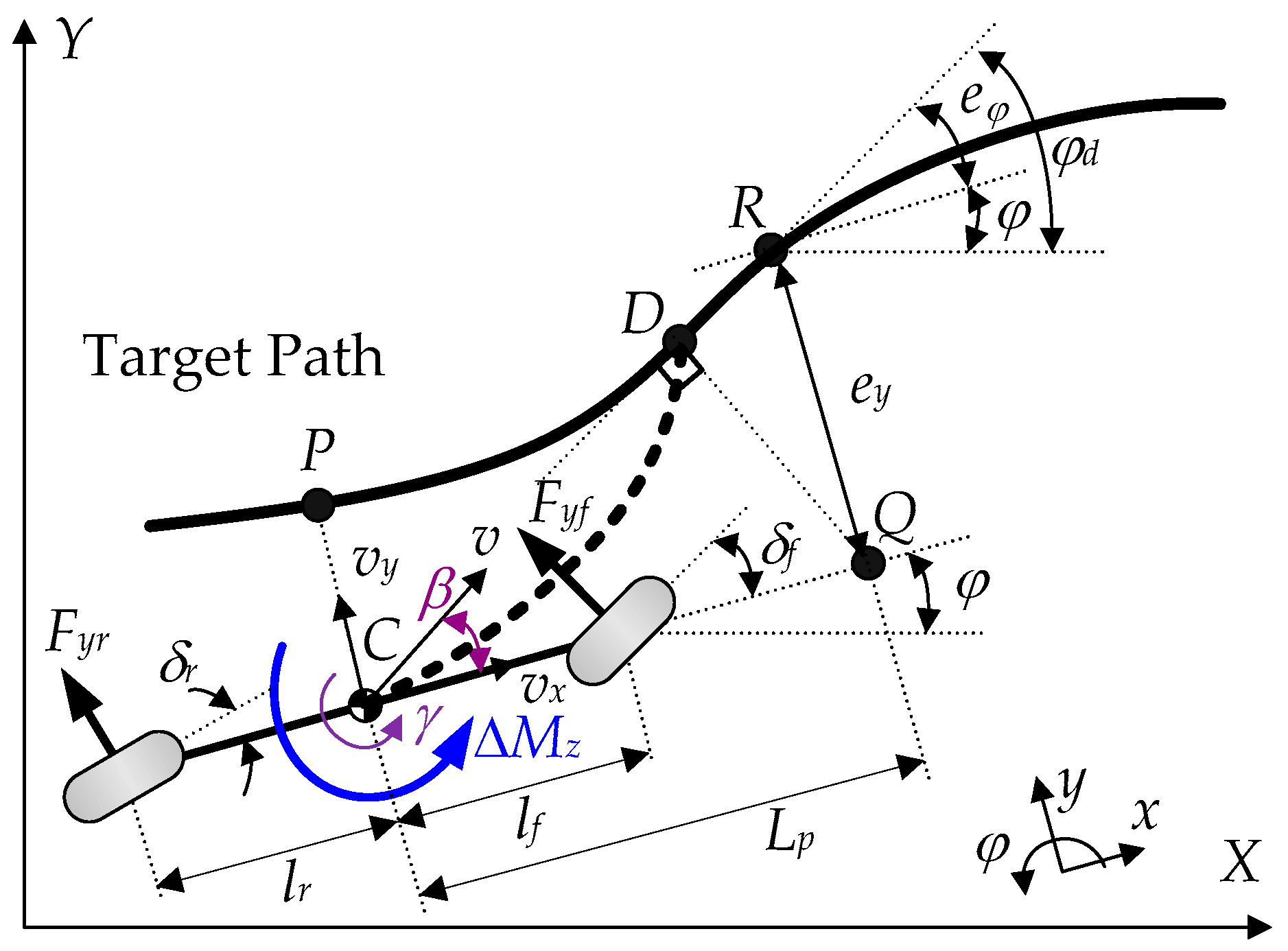
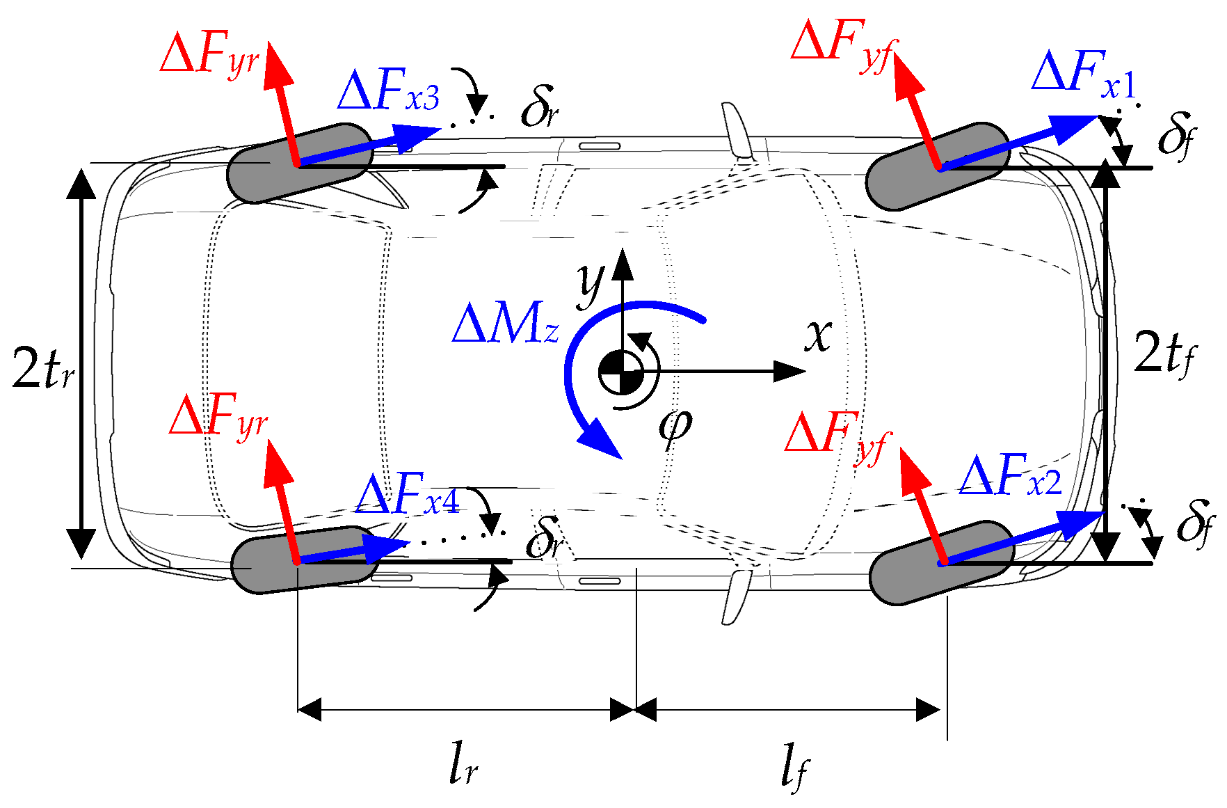
2.1. Derivation of State-Space Model

Following the literature of PTC, a 2-DOF bicycle model is selected as vehicle one. Figure 2 shows the coordinates and variables of the bicycle model and the target path used for path tracking [12,13]. This model describes the lateral and yaw motions of a vehicle under the assumption that v_x is constant. With γ and β as a state variable, the equations of motions for the model are obtained as (1) [42,43]. At the front and rear wheels, the slip angles, α_f and α_r, are defined as (2) under the assumption that tan⁻¹(θ) ≈ θ for small θ. The lateral tire forces, F_yf and F_yr, at the front and rear wheels are calculated as (3) under the assumption that the lateral tire force is linear with respect to the slip angle. By combining (1), (2), and (3), the linear state-space equations for the bicycle model are derived as (4).

$$\left\{\begin{array}{l}m{v}_x\left(\dot{\beta }+\gamma \right)=F_{yf}+F_{yr}\\ I_z\dot{\gamma }=l_f{F}_{yf}-l_r{F}_{yr}+\Delta M_z\end{array}\right.$$

(1)

$$\left\{\begin{array}{l}{\alpha }_f={\delta }_f-{\tan }^{-1}\left(\beta +\frac{l_f\gamma }{v_x}\right)\approx {\delta }_f-\beta -\frac{l_f\gamma }{v_x}\\ {\alpha }_r={\delta }_r-{\tan }^{-1}\left(\beta -\frac{l_r\gamma }{v_x}\right)\approx {\delta }_r-\beta +\frac{l_r\gamma }{v_x}\end{array}\right.$$

(2)

$$F_{yf}=2C_f{\alpha }_f,\hspace{1em}{F}_{yr}=2C_r{\alpha }_r$$

(3)

$$\begin{array}{l}\dot{\beta }=\left(\frac{{\varsigma }_1}{m{v}_x}\right)\beta +\left(\frac{{\varsigma }_2}{m{v}_x^2}-1\right)\gamma +\frac{C_f}{m{v}_x}{\delta }_f+\frac{C_f}{m{v}_x}{\delta }_r\\ \dot{\gamma }=\left(\frac{{\varsigma }_2}{I_z}\right)\beta +\left(\frac{{\varsigma }_3}{I_z{v}_x}\right)\gamma +\frac{l_f{C}_f}{I_z}{\delta }_f-\frac{l_r{C}_r}{I_z}{\delta }_r+\frac{\Delta M_z}{I_z}\\ {\varsigma }_1=-C_f-C_r,\hspace{0.33em}{\varsigma }_2=-C_f{l}_f+C_r{l}_r,\hspace{0.33em}{\varsigma }_3=-l_f^2{C}_f-l_r^2{C}_r\end{array}$$

(4)

In the literature of PTC, the lateral offset and heading errors, e_y and e_φ, have been defined at point P in Figure 2. In this paper, a lookahead or preview function is introduced to improve the path-tracking performance when calculating those errors [12,21,22,24,34,38,40]. The lookahead or preview distance L_p is calculated using (5). In (5), t_p is the preview interval or preview time, which acts as a velocity gain. In Figure 2, point C is located at the center of gravity (C.G.) of a vehicle. With L_p, the lookahead point Q and the point R on the target path are obtained. At point R, the time-derivative of e_y and e_φ is calculated as (6) under the assumption that e_φ is smaller than 10° and its consequence is sine_φ ≈ e_φ.

$$L_p=t_p\cdot v_x$$

(5)

$$\left\{\begin{array}{l}{\dot{e}}_y=v_x\sin e_{\phi }-v_x\beta -L_p\gamma \approx v_x{e}_{\phi }-v_x\beta -L_p\gamma \\ {\dot{e}}_{\phi }={\dot{\phi }}_d-\dot{\phi }=v_x\chi -\gamma \end{array}\right.$$

(6)

With the state variables of e_y, e_φ, β, and γ, the state vector, x, the disturbance, w, and the control input, u, are defined as (7). From (4), (6), and (7), the state-space equation for PTC and VSC is obtained as (8) [21,22,24]. In (8), the system, disturbance, and input matrices, A, B₁, and B₂, are defined in (9).

$$x={\left[\begin{array}{cccc}{e}_y& e_{\phi }& \beta & \gamma \end{array}\right]}^T,\hspace{1em}w=\chi ,\hspace{1em}u={\left[\begin{array}{ccc}{\delta }_f& {\delta }_r& \Delta M_z\end{array}\right]}^T$$

(7)

$$\dot{x}=Ax+B_{1}w+B_{2u}$$

(8)

$$A=\left[\begin{array}{cccc}0& v_x& -v_x& -L_p\\ 0& 0& 0& -1\\ 0& 0& \frac{{\varsigma }_1}{m{v}_x}& \frac{{\varsigma }_2}{m{v}_x^2}-1\\ 0& 0& \frac{{\varsigma }_2}{I_z}& \frac{{\varsigma }_3}{I_z{v}_x}\end{array}\right],\hspace{1em}{B}_1=\left[\begin{array}{c}0\\ v_x\\ 0\\ 0\end{array}\right],\hspace{1em}{B}_2=\left[\begin{array}{lll}0\hfill & 0\hfill & 0\hfill \\ 0\hfill & 0\hfill & 0\hfill \\ \frac{C_f}{m{v}_x}\hfill & \frac{C_r}{m{v}_x}\hfill & 0\hfill \\ \frac{l_f{C}_f}{I_z}\hfill & -\frac{l_r{C}_r}{I_z}\hfill & \frac{1}{I_z}\hfill \end{array}\right]$$

(9)

The control input u defined in (7) is composed of δ_f, δ_r, and ∆M_z. From those elements of the control input u, four control inputs, u₁, u₂, u₃, and u₄, are set as (10), which correspond to the input configurations, IC#1, IC#2, IC#3, and IC#4, respectively [13]. According to four control inputs, u₁, u₂, u₃, and u₄, the input matrices, B₂₁, B₂₂, B₂₃, and B₂₄, are defined in (10) from (9) [13]. In (10), B₂(k) represents the k-th column of the matrix B₂ in (9). As shown in (10), δ_f is available for all ICs. δ_r is available for IC#2, IC#3, and IC#4. For IC#3 and IC#4 with ∆M_z, 4WIB and 4WID are available when generating ∆M_z. ∆M_z in IC#3 and IC#4 should be converted into δ_r and the braking and traction torques (T_Bi and T_Di) at each wheel using a control allocation procedure. For IC#4, RWS, i.e., δ_r, is not used when converting ∆M_z into tire forces because it is already included in the control input, u₄. In this paper, it is assumed that T_Bi and T_Di are generated via 4WIB and 4WID, respectively. In this paper, IC#1 and IC#2 are used as a baseline of PTC#1. Moreover, IC#1 is used as a steering angle generator for PTC#2.

$$\left\{\begin{array}{lll}{u}_1={\delta }_f\hfill & B_{21}=\left[B_2\left(1\right)\right]\hfill & \mathrm{for}\hspace{0.33em}IC\#1\hfill \\ u_2={\left[\begin{array}{cc}{\delta }_f& {\delta }_r\end{array}\right]}^T\hfill & B_{22}=\left[\begin{array}{cc}{B}_2\left(1\right)& B_2\left(2\right)\end{array}\right]\hfill & \mathrm{for}\hspace{0.33em}IC\#2\hfill \\ u_3={\left[\begin{array}{cc}{\delta }_f& \Delta M_z\end{array}\right]}^T\hfill & B_{23}=\left[\begin{array}{cc}{B}_2\left(1\right)& B_2\left(3\right)\end{array}\right]\hfill & \mathrm{for}\hspace{0.33em}IC\#3\hfill \\ u_4={\left[\begin{array}{ccc}{\delta }_f& {\delta }_r& \Delta M_z\end{array}\right]}^T\hfill & B_{24}=\left[\begin{array}{ccc}{B}_2\left(1\right)& B_2\left(2\right)& B_2\left(3\right)\end{array}\right]\hfill & \mathrm{for}\hspace{0.33em}IC\#4\hfill \end{array}\right.$$

(10)

2.2. Design of LQR for PTC#1 and PTC#2

LQ objective functions, J₁, J₂, J₃, and J₄, for input configurations, IC#1, IC#2, IC#3, and IC#4, of (10) are provided in (11), respectively. As shown in (11), the first two terms of J₀ including e_y and e_φ represent the path-tracking objective, and the last two terms of J₀ including β and γ represent the vehicle stability objective, which can be divided into lateral stability and yaw rate tracking. In this manner, PTC and VSC are integrated into a single control framework. J₁, J₂, J₃, and J₄ can be converted into the vector matrix form of (12). In (12), the matrices Q and R_i are provided as (13). In (11) and (13), the weight ρ_i is set using Bryson’s rule, (14), where ξ_i is the maximum allowable value of the corresponding term [44]. The actual tuning procedure for path tracking and vehicle stability is carried out by adjusting ξ_i. The control input u_i of IC#i in LQR is calculated as (15), where S_i is the solution of the Riccati equation for IC#i.

$$\begin{array}{l}{J}_0={\displaystyle {\int }_0^{\infty }\left\{{\rho }_1{e}_y^2+{\rho }_2{e}_{\phi }^2+{\rho }_3{\beta }^2+{\rho }_4{\gamma }^2\right\}dt}\hspace{1em}\\ \left\{\begin{array}{ll}{J}_1=J_0+{\displaystyle {\int }_0^{\infty }\left({\rho }_5{\delta }_f^2\right)dt}\hfill & \mathrm{for}\hspace{0.33em}IC\#1\hfill \\ J_2=J_0+{\displaystyle {\int }_0^{\infty }\left({\rho }_5{\delta }_f^2+{\rho }_6{\delta }_r^2\right)dt}\hfill & \mathrm{for}\hspace{0.33em}IC\#2\hfill \\ J_3=J_0+{\displaystyle {\int }_0^{\infty }\left({\rho }_5{\delta }_f^2+{\rho }_7\Delta M_z^2\right)dt}\hfill & \mathrm{for}\hspace{0.33em}IC\#3\hfill \\ J_4=J_0+{\displaystyle {\int }_0^{\infty }\left({\rho }_5{\delta }_f^2+{\rho }_6{\delta }_r^2+{\rho }_7\Delta M_z^2\right)dt}\hfill & \mathrm{for}\hspace{0.33em}IC\#4\hfill \end{array}\right.\end{array}$$

(11)

$$J_i=={\displaystyle {\int }_0^{\infty }{\left[\begin{array}{c}x\\ u_i\end{array}\right]}^T\left[\begin{array}{cc}Q& 0\\ 0& R_i\end{array}\right]\left[\begin{array}{c}x\\ u_i\end{array}\right]dt},\hspace{0.33em}i=1,\cdots ,4$$

(12)

$$Q=diag\left({\rho }_1,{\rho }_2,{\rho }_3,{\rho }_4\right),\hspace{1em}\left\{\begin{array}{ll}{R}_1={\rho }_5\hfill & \mathrm{for}\hspace{0.33em}IC\#1\hfill \\ R_2=diag\left({\rho }_5,{\rho }_6\right)\hfill & \mathrm{for}\hspace{0.33em}IC\#2\hfill \\ R_3=diag\left({\rho }_5,{\rho }_7\right)\hfill & \mathrm{for}\hspace{0.33em}IC\#3\hfill \\ R_4=diag\left({\rho }_5,{\rho }_6,{\rho }_7\right)\hfill & \mathrm{for}\hspace{0.33em}IC\#4\hfill \end{array}\right.$$

(13)

$${\rho }_i=\frac{1}{{\xi }_i^2}$$

(14)

$$u_i=K_{i}x=-R_i^{-1}{B}_{2i}^T{S}_{i}x,\hspace{0.33em}i=1,\cdots ,4$$

(15)

2.3. Derivation of the Reference Yaw Rate for PTC#2 and PTC#3

There are two methods that have been used to derive the reference yaw rate, γ_ref. The first method uses the FWS angle and the bicycle model provided in (4), and the second is to use a target path. In the first method, γ_ref is calculated to γ_s as provided in (16) [12,18,19,31,32,33,35,36,37,42]. The front steering angle, δ_f, is obtained from the LQR with IC#1 of PTC#1. In (16), K_γ is the steady-state yaw rate gain. In the previous study, it was shown that K_γ can be tuned regardless of C_f, C_r, m, and v_x for the purpose of enhancing path-tracking performance [11]. Generally, γ_s is bounded by (17) [43].

$${\gamma }_s=\frac{2\cdot C_f\cdot C_r\cdot \left(l_f+l_r\right)\cdot v_x}{2\cdot C_f\cdot C_r\cdot {\left(l_f+l_r\right)}^2+m\cdot v_x^2\cdot \left(l_r\cdot C_r-l_f\cdot C_f\right)}\cdot {\delta }_f=K_{\gamma }\cdot {\delta }_f$$

(16)

$${\gamma }_s\le 0.85\frac{\mu g}{v_x}$$

(17)

In the second method, γ_ref is obtained from a target path without a vehicle model [11,38,39,40]. The typical method for this purpose is to derive γ_p from Figure 1 as provided in (18) [38]. Another method is to use a polynomial interpolation, which is adopted in this paper [11,12,39]. Figure 1 shows the desired and target paths and three points, C, D, and Q. Let the coordinate values of the points, C, D, and Q, be (x₀,y₀), (x₁,y₁), and (x₂,y₂), respectively. In Figure 1, the desired path is marked as a dashed bold line, connecting points C and D. To derive γ_ref for PTC, the curvature of the desired path should be calculated. Under the assumption that point D is close enough to the vehicle, the desired path is represented with a second-order polynomial, as provided in (19). Three coefficients, a₁, a₂, and a₃, of the polynomial are determined using (20) from the positions of the points C and D and the slope at the point C. With the coefficients of the polynomial, the curvature χ_d at point C is calculated as in (21). Finally, γ_ref for PTC is calculated into γ_d as in (22) [11,39]. In (22), the preview interval K_p plays an identical role to K_γ in (16). In this paper, K_p is set to 1 and γ_d is also limited by (17).

$${\gamma }_p=\frac{2}{t_p}\left\{{\tan }^{-1}\left(\frac{e_y}{L_p}\right)-\beta \right\}$$

(18)

$$y(x)=a_1{x}^2+a_{2}x+a_3$$

(19)

$$\left[\begin{array}{c}{a}_1\\ a_2\\ a_3\end{array}\right]={\left[\begin{array}{ccc}{x}_0{}^2& x_0& 1\\ x_1{}^2& x_1& 1\\ 2x_0& 1& 0\end{array}\right]}^{-1}\left[\begin{array}{c}{y}_0\\ y_1\\ y^{\prime }(x_0)\end{array}\right]$$

(20)

$${\chi }_d=\frac{y^{″}\left(x_0\right)}{{\left\{1+y^{\prime }{\left(x_0\right)}^2\right\}}^{3/2}}=\frac{2a_1}{{\left\{1+{\left(2a_1{x}_0+a_2\right)}^2\right\}}^{3/2}}$$

(21)

$${\gamma }_d=K_p\cdot v_x\cdot {\chi }_d$$

(22)

2.4. Design of Yaw Rate Tracking Controller for PTC#2 and PTC#3

To make γ follow the reference yaw rates, γ_s or γ_d, it is necessary to calculate ΔM_z. The yaw rate error, γ_e, is defined as (23), where this is set to the error surface, s. To make the surface asymptotically converge to zero, the condition of (24) should be satisfied [11,12,18,19,39]. By combining (1), (23), and (24), ∆M_z is computed as (25). In this paper, K_c is set to 5.

$$s={\gamma }_e=\gamma -{\gamma }_{ref}$$

(23)

$$\dot{s}=-K_{c}s\hspace{1em}\left(K_c>0\right)$$

(24)

$$\Delta M_z=I_z\cdot {\dot{\gamma }}_d-l_f{F}_{yf}+l_r{F}_{yr}-I_z\cdot K_c\cdot \left(\gamma -{\gamma }_{ref}\right)$$

(25)

2.5. Control Allocation with WLS for PTC#1, PTC#2, and PTC#3

The control yaw moment, ΔM_z, is obtained commonly from PTC#1, PTC#2, and PTC#3. Once ∆M_z is obtained, it should be converted into the longitudinal of wheels, which are generated using the actuators, i.e., 4WIB and 4WID, via a control allocation. For control allocation, a weighted least square (WLS)-based method is adopted in this paper [20,21,22,23,24,25,26,27,28,29,30,31,32,33,34,35,36,37].

Figure 3 shows tire forces at each wheel and ∆M_z, when ∆M_z is positive [13,18,19,45]. In Figure 3, ∆F_yf and ∆F_yr are the lateral tire forces of the front and rear wheels, which are generated via FWS and RWS, respectively. ∆F_x1, ∆F_x2, ∆F_x3, and ∆F_x4 are the longitudinal tire forces generated via 4WID and 4WIB. If ∆F_i is positive, it is generated as the traction torque T_Di via 4WID. Otherwise, it is generated as the braking torque T_Bi via 4WIB. These six tire forces should be determined to generate ∆M_z. The WLS-based method is used for this purpose.

From the geometric relationship shown in Figure 3, the equilibrium condition among ∆M_z and tire forces is obtained as (26) [11,12,18,19,39]. In (26), the elements of the vector p are provided in (27).

$$\underset{p}{\underbrace{\left[\begin{array}{cccccc}{p}_1& p_2& p_3& p_4& p_5& p_6\end{array}\right]}}\underset{q}{\underbrace{\left[\begin{array}{c}\Delta F_{yf}\\ \Delta F_{yr}\\ \Delta F_{x1}\\ \Delta F_{x2}\\ \Delta F_{x3}\\ \Delta F_{x4}\end{array}\right]}}=\Delta M_z$$

(26)

$$\left\{\begin{array}{l}{p}_1=-2l_f\cos {\delta }_f,\hspace{1em}{p}_2=2l_r\cos {\delta }_r,\\ p_3=-l_f\sin {\delta }_f+t_f\cos {\delta }_f,\hspace{1em}{p}_4=-l_f\sin {\delta }_f-t_f\cos {\delta }_f,\\ p_5=l_r\sin {\delta }_r+t_r\cos {\delta }_r,\hspace{1em}\hspace{0.33em}{p}_6=l_r\sin {\delta }_r-t_r\cos {\delta }_r\end{array}\right.$$

(27)

The objective function of WLS is defined with the quadratic form as in (28). In (28), μF_zi represents the radius of the friction circle at the wheel i. Assuming that the road surface is flat, it can be easily estimated using acceleration signals measured by sensors [46]. In (28), κ is the vector of virtual weights, κ_i, which is used to select the combination of actuators [39,47,48]. The equality constraint (26) is converted into the quadratic form (29). In the previous study, (26) must be satisfied in order to generate ∆M_z. The objective function (28) and the constraint (29) are combined into a single objective one (30), with the Lagrange multiplier, ζ. In (30), ζ should be set to 1 or higher. In this paper, ζ is set to 10. Otherwise, the constraint (26) is not satisfied. The optimum of (30) is algebraically obtained as (31) by differentiating (30) with respect to q [13].

$$\begin{array}{l}{J}_E=\frac{{\kappa }_1\Delta F_{yf}^2+{\kappa }_3\Delta F_{x1}^2}{{\left(\mu F_{z1}\right)}^2}+\frac{{\kappa }_1\Delta F_{yf}^2+{\kappa }_4\Delta F_{x2}^2}{{\left(\mu F_{z2}\right)}^2}+\frac{{\kappa }_2\Delta F_{yf}^2+{\kappa }_5\Delta F_{x3}^2}{{\left(\mu F_{z3}\right)}^2}+\frac{{\kappa }_2\Delta F_{yf}^2+{\kappa }_6\Delta F_{x4}^2}{{\left(\mu F_{z4}\right)}^2}\hspace{0.33em}=p^{T}Wp\\ W=\mathrm{diag}\left[\frac{1}{{\left(\mu F_{z1}\right)}^2}+\frac{1}{{\left(\mu F_{z2}\right)}^2},\frac{1}{{\left(\mu F_{z3}\right)}^2}+\frac{1}{{\left(\mu F_{z4}\right)}^2},\frac{1}{{\left(\mu F_{z1}\right)}^2},\frac{1}{{\left(\mu F_{z2}\right)}^2},\frac{1}{{\left(\mu F_{z3}\right)}^2},\frac{1}{{\left(\mu F_{z4}\right)}^2}\right]\kappa \hspace{1em}\\ \kappa =\mathrm{diag}\left[\begin{array}{cccccc}{\kappa }_1& {\kappa }_2& {\kappa }_3& {\kappa }_4& {\kappa }_5& {\kappa }_6\end{array}\right]\end{array}$$

(28)

$$J_{EC}={\left(pq-\Delta M_z\right)}^T\left(pq-\Delta M_z\right)$$

(29)

$$J_{CA}=J_E+\zeta \cdot J_{EC}=q^{T}Wq+\zeta {\left(pq-\Delta M_z\right)}^T\left(pq-\Delta M_z\right)$$

(30)

$$q_{opt}=\zeta {\left(W+\eta p^{T}p\right)}^{-1}{p}^T\Delta M_z$$

(31)

When applying WLS for control allocation with ∆M_z, arbitrary actuator combinations composed of FWS, RWS, 4WS, 4WIB, and 4WID can be set according to a particular input configuration. For example, if u₄ of IC#4 in (10) is selected as a control input, only 4WID and 4WIB are available to be used in generating ∆M_z because δ_f and δ_r of FWS, RWS, and 4WS are already determined using LQR. To reflect this fact, the virtual weights, κ_i, can be set according to a particular combination of multiple actuators, FWS, RWS, 4WS, 4WIB, and 4WID [39,47,48].

The vectors of virtual weights corresponding to steering actuators, i.e., FWS, RWS, and 4WS, are provided in (32). Initially, all the virtual weights are set to 1. In (32), ε is 10⁻⁴ and the terms denoted by ● have no effect on the steering actuators. The first and second terms of κ in (32) correspond to ∆F_yf and ∆F_yr, respectively, which are converted into the front and rear steering angles. If the first term of κ is set to ε, then only ∆F_yf is generated via WLS. This is shown in the first row of (32).

$$\left\{\begin{array}{l}\begin{array}{cc}\mathrm{FWS}:& \kappa =\mathrm{diag}\left[\begin{array}{cccccc}\epsilon & 1& •& •& •& •\end{array}\right]\end{array}\\ \begin{array}{cc}\mathrm{RWS}:& \kappa =\mathrm{diag}\left[\begin{array}{cccccc}1& \epsilon & •& •& •& •\end{array}\right]\end{array}\\ \begin{array}{cc}4\mathrm{WS}:& \kappa =\mathrm{diag}\left[\begin{array}{cccccc}\epsilon & \epsilon & •& •& •& •\end{array}\right]\end{array}\end{array}\right.$$

(32)

The vectors of virtual weights representing 4WIB and 4WID are provided in (33). Figure 3 shows the fact that only ∆F_x2 and ∆F_x4 should be generated if ∆M_z is negative and 4WIB is available. This is represented by the second row of the first term, 4WIB in (33). If 4WIB and 4WID are available for generating ∆M_z, no constraints are imposed on the longitudinal forces, which is represented by the last row of (33), i.e., 4WID + 4WIB. The virtual weights provided in (32) and (33) can be set according to combinations of actuators available for the purpose of generating ∆M_z.

$$\left\{\begin{array}{l}\begin{array}{cc}4\mathrm{WID}:& \left\{\begin{array}{l}\kappa =\mathrm{diag}\left[\begin{array}{cccccc}•& •& 1& \epsilon & 1& \epsilon \end{array}\right]\hspace{1em}\mathrm{if}\hspace{0.33em}\Delta M_z>0\\ \kappa =\mathrm{diag}\left[\begin{array}{cccccc}•& •& \epsilon & 1& \epsilon & 1\end{array}\right]\hspace{1em}\mathrm{if}\hspace{0.33em}\Delta M_z<0\end{array}\right.\end{array}\\ \begin{array}{cc}4\mathrm{WIB}:& \left\{\begin{array}{l}\kappa =\mathrm{diag}\left[\begin{array}{cccccc}•& •& \epsilon & 1& \epsilon & 1\end{array}\right]\hspace{1em}\mathrm{if}\hspace{0.33em}\Delta M_z>0\\ \kappa =\mathrm{diag}\left[\begin{array}{cccccc}•& •& 1& \epsilon & 1& \epsilon \end{array}\right]\hspace{1em}\mathrm{if}\hspace{0.33em}\Delta M_z<0\end{array}\right.\end{array}\\ \begin{array}{cc}4\mathrm{WID}+4\mathrm{WIB}:& \kappa =\mathrm{diag}\left[\begin{array}{cccccc}•& •& \epsilon & \epsilon & \epsilon & \epsilon \end{array}\right]\end{array}\end{array}\right.$$

(33)

In this paper, T_Bi and T_Di at the wheel i are calculated from ∆F_x1, ∆F_x2, ∆F_x3, and ∆F_x4, determined via the WLS-based method, i.e., q_opt in (31). Following the sign of ∆F_xi, T_Bi, and T_Di at the wheel i are calculated as (34), respectively [13].

$$\left.\left\{\begin{array}{l}{T}_{Bi}\hspace{0.33em}\hspace{0.33em}\mathrm{if}\hspace{0.33em}\Delta F_{xi}<0\hfill \\ T_{Di}\hspace{0.33em}\hspace{0.33em}\mathrm{if}\hspace{0.33em}\Delta F_{xi}>0\hfill \end{array}\hspace{0.33em}\right.\right\}=h\left(\frac{r_{wi}\Delta F_{xi}}{{\upsilon }_i},{\omega }_i\right),\hspace{0.33em}\hspace{0.33em}i=1,\cdots ,4$$

(34)

δ_f and δ_r are calculated from ∆F_yf and ∆F_yr obtained in q_opt and the definitions of (2) and (3). The definition of the lateral tire force (3) is rewritten as (35). In (35), σ is the parameter representing the magnitude of the cornering stiffness, C_i [34]. In this paper, σ is set to 6. For 4WS, δ_f and δ_r are calculated as (36) by combining (2) with (35) [13,49]. In these formulations, β is needed. However, it is hard to measure. For this reason, an extended Kalman Filter is adopted to estimate β [50] in this paper.

$${\varphi }_i=-\frac{\Delta F_{yi}}{\sigma C_i},\hspace{1em}i=f,r$$

(35)

$$\left\{\begin{array}{l}{\delta }_f=-{\alpha }_f+\beta +\frac{l_f\gamma }{v_x}=-{\varphi }_f+\beta +\frac{l_f\gamma }{v_x}\\ {\delta }_r=-{\alpha }_r+\beta -\frac{l_r\gamma }{v_x}=-{\varphi }_r+\beta -\frac{l_r\gamma }{v_x}\end{array}\right.$$

(36)

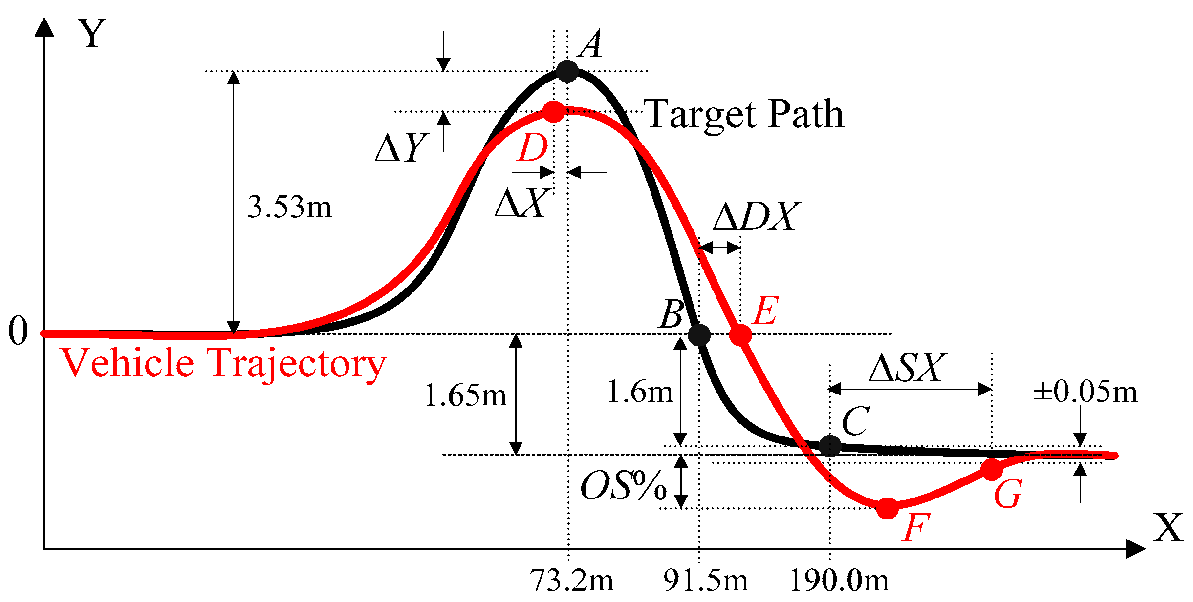
3. Performance Measures for Path Tracking and Vehicle Stability

In the literature of PTC, e_y and e_φ have been used to represent the path-tracking performance. Different from the literature on PTC, a double lane change maneuver for collision avoidance is adopted as a target path in this paper [11,12,13,20,26,27,37]. This path has been used to measure the reachability and agility of a path-tracking controller [12,13]. Figure 4 shows the target path and vehicle trajectory. From the points on the target path and the vehicle trajectory in Figure 4, five measures standing for path-tracking performance are defined as (37): the peak’s center offset, ∆X, the peak’s lateral offset, ∆Y, the percentage over-shoot, OS%, the response delay, ∆DX, and the settling delay, ∆SX. These measures are illustrated in Figure 4. In (37), the subscripts X and Y represent the x- and y-positions of the point ●, respectively. Basically, the smaller the absolute magnitudes of these measures, the better the path-tracking performance.

$$\left\{\begin{array}{l}\Delta X=D_X-A_X=D_X-73.20\\ \Delta Y=D_Y-A_Y=D_Y-3.53\\ \Delta DX=E_X-B_X=E_X-91.50\\ \Delta SX=G_X-C_X=G_X-190.00\\ OS\%=\frac{\left|F_Y\right|-1.65}{1.65+3.53}\times 100\end{array}\right.$$

(37)

In Figure 4, ∆X and ∆Y represent the agility and the reachability, respectively. In this paper, if ∆Y is larger than −0.05 m, it is regarded that the path-tracking performance of a controller is satisfactory. OS% stands for lateral damping, which represents agility. In this paper, it is satisfactory if OS% is less than 16%, which is equal to the overshoot of 0.85 m. ∆DX stands for the response delay, which stands for the agility of the longitudinal motion. ∆SX can be regarded as the settling time, which stands for the convergence speed of the vehicle’s lateral motion to a target value of y-position. In this paper, it is satisfactory if ∆SX is less than 16 m. Generally, if OS% is near 1% under the condition that ∆Y is larger than −0.05 m, the best performance is achieved. Detailed explanations of these measures can be found in [12,13].

As mentioned earlier, VSC stands for yaw rate tracking and lateral stability. Generally, yaw rate tracking performance is measured with the yaw rate error γ_e and lateral stability performance is measured with β. It has been regarded that lateral stability performance is satisfactory if β is less than 3° [51]. Let us denote the maximum absolute value of β to be MASSA. The side-slip angular rate, combined with β, has been also used as a measure of lateral stability. Let us denote the maximum absolute value of the side-slip angular rate to be MASSAR [12].

4. Simulation and Discussion

4.1. Simulation Environment

A simulation was conducted to compare three controllers, PTC#1, PTC#2, and PTC#3, on low-friction roads in terms of path-tracking performance. These controllers were implemented using MATLAB/Simulink (2019a) and connected with the vehicle simulation software CarSim 8 [52]. The configuration of MATLAB/Simulink and CarSim is provided in Figure 1. In Figure 1, the autonomous electrical vehicles with FWS/4WS, 4WID, and 4WIB are replaced by CarSim, and the other parts are implemented with MATLAB/Simulink. A target path in Figure 4 was selected as a test scenario. In the simulation, the built-in F-segment sedan model provided in the CarSim software was selected [52]. From the model, the parameters of the bicycle model are provided in

Table 1. Parameter of 2-DOF bicycle model obtained from F-segment sedan in CarSim.

Parameter	Value	Parameter	Value
ms	1823 kg	Iz	6286 kg·m2
Cf	42,000 N/rad	Cr	62,000 N/rad
lf	1.27 m	lr	1.90 m
tf	0.80 m	tr	0.80 m

. In Table 1, the cornering stiffness, C_f and C_r, are obtained from simulation in CarSim by comparing β and γ of CarSim and the state-space model under a step steering maneuver. The steering actuators of FWS and 4WS were modeled as the first-order system with a time constant of 0.05. 4WIB and 4WID were modeled as the first-order system with a time constant of 0.1. The initial v_x and μ were set to 60 km/h and 0.4, respectively. The speed controller provided in CarSim was applied upon driving to maintain a constant speed, which means that K_γ is maintained as constant as possible.

In real vehicles, the magnitude of ∆M_z is limited by the maximum tire forces and road surface friction. To reflect this fact, it is necessary to set a bound on ∆M_z. For this purpose, ∆M_z is limited to a certain value after calculating it using LQR. For example, IC#4 of PTC#1 can use the smallest ∆M_z among the input configurations because only the longitudinal tire forces are available for control allocation. A detailed description of how to select the limit of ∆M_z can be found in Reference [13].

The tuning was carried out by trial and error such that ∆Y is larger than −0.05 m and OS% is near 0.9, which gives the smallest ∆DX and ∆SX. The most important tuning parameters are the velocity gain t_p, ζ₁ and ζ₂ in (14). If RWS is adopted, the weight on RWS, i.e., ζ₆ in (14), should be set to a small value such that β is smaller than 2.5°.

4.2. Simulation with PTC#1

The first simulation was carried out with PTC#1. For IC#1, IC#2, IC#3, and IC#4, several actuator combinations composed of RWS, 4WS, 4WID, and 4WIB were used for control allocation. The tuning parameters of PTC#1 are t_p and ζ_i as provided in (5) and (14), respectively. The simulation results of PTC#1 are summarized in

Table 2. Summary of the simulation results for IC#1, IC#2, IC#3, and IC#4 of PTC#1.

	Actuator Combinations	∆X (m)	∆Y (m)	OS%	∆DX (m)	∆SX (m)	MASSA (deg)	MASSAR (deg/s)
IC#1	FWS	1.57	0.002	1.0	8.98	4.84	0.58	13.13
IC#2	4WS	1.61	0.013	0.9	9.12	5.06	1.67	14.73
IC#3	FWS + 4WID	1.19	−0.035	0.9	8.91	4.64	0.59	13.34
	+4WIB	1.29	−0.024	1.0	8.80	4.63	0.59	0.59
	+4WID + 4WIB	1.30	−0.015	1.0	8.71	4.59	0.59	13.22
	FWS + RWS	1.25	−0.003	0.9	8.74	4.58	1.36	13.84
	+4WID	1.35	0.000	1.0	8.87	4.70	1.35	14.02
	+4WIB	1.59	0.000	1.0	9.17	5.01	1.15	13.11
	+4WID + 4WIB	1.60	0.004	0.9	9.13	4.99	1.13	13.30
IC#4	+4WID	1.45	−0.002	0.9	9.21	5.07	2.09	15.30
	+4WIB	1.48	0.004	1.0	9.10	5.04	2.08	15.08
	+4WID + 4WIB	1.49	0.010	0.9	9.04	5.02	1.96	15.07

. The velocity gains and weights of the LQ objective function are provided in

Table 3. Velocity gains and weights of LQ objective function for IC#1, IC#2, IC#3, and IC#4 of PTC#1.

	Actuator Combinations	tp	ξ1	ξ2	ξ3	ξ4	ξ5	ξ6	ξ7
IC#1	FWS	0.60	0.5600	5.000	0.30	10.00	0.05	-	-
IC#2	4WS	0.60	0.5500	0.700	0.30	10.0	0.05	0.005	-
IC#3	FWS + 4WID	1.19	0.0518	0.005	0.10	0.10	0.03	-	50.0
	+4WIB	1.29	0.0532	0.005	0.10	0.10	0.03	-	50.0
	+4WID + 4WIB	1.30	0.0572	0.005	0.10	0.10	0.03	-	50.0
	FWS + RWS	1.25	0.0662	0.005	0.10	0.10	0.03	-	50.0
	+4WID	1.35	0.0644	0.005	0.10	0.10	0.03	-	50.0
	+4WIB	1.59	0.0585	0.005	0.10	0.10	0.03	-	50.0
	+4WID + 4WIB	1.60	0.0598	0.005	0.10	0.10	0.03	-	50.0
IC#4	+4WID	1.45	0.0566	0.005	0.10	0.10	0.03	0.001	50.0
	+4WIB	1.48	0.0569	0.005	0.10	0.10	0.03	0.001	50.0
	+4WID + 4WIB	1.49	0.0606	0.005	0.10	0.10	0.03	0.001	50.0

. As shown in Table 2, there are few differences among the input configurations and actuator combinations in terms of path-tracking performance. A notable feature is that the use of RWS increases MASSA. This is caused by the fact that RWS steers the rear wheels along the identical direction to the front wheels. These results are identical to those of [13].

For IC#3, ∆M_z is added to IC#1, i.e., FWS. As shown in Table 2, the ∆X of IC#3 is reduced by adding ∆M_z to IC#1. Especially, RWS and 4WID have a large effect on the reduction in ∆X. Among them, 4WID is preferred to RWS because 4WID does not increase MASSA. On the contrary, IC#4 adds ∆M_z to IC#2, i.e., 4WS. As shown in Table 2, there are few effects of adding ∆M_z to IC#2 on path-tracking performance although ∆X is slightly decreased by adding ∆M_z. In Table 2, the actuator combinations with RWS in IC#3 are equivalent to those of IC#4. As shown in Table 2, the former is better than the latter in terms of path-tracking performance. This fact means that the control allocation with multiple actuators for 4WS is not effective. Instead, it is desirable to add ∆M_z to IC#1 and use control allocation with multiple actuators. Besides the increase in MASSA and the reduction in ∆X, there are few effects of adding ∆M_z to IC#1 or IC#2. Figure 5, Figure 6 and Figure 7 show the trajectories and side-slip angles of every input configuration and actuator combination provided in Table 2. As shown in these figures, there are little differences among trajectories. On the contrary, only the side-slip angles are different from one another. From these results, it can be concluded that it is desirable to not use the multiple actuators needed to generate ∆M_z for path tracking.

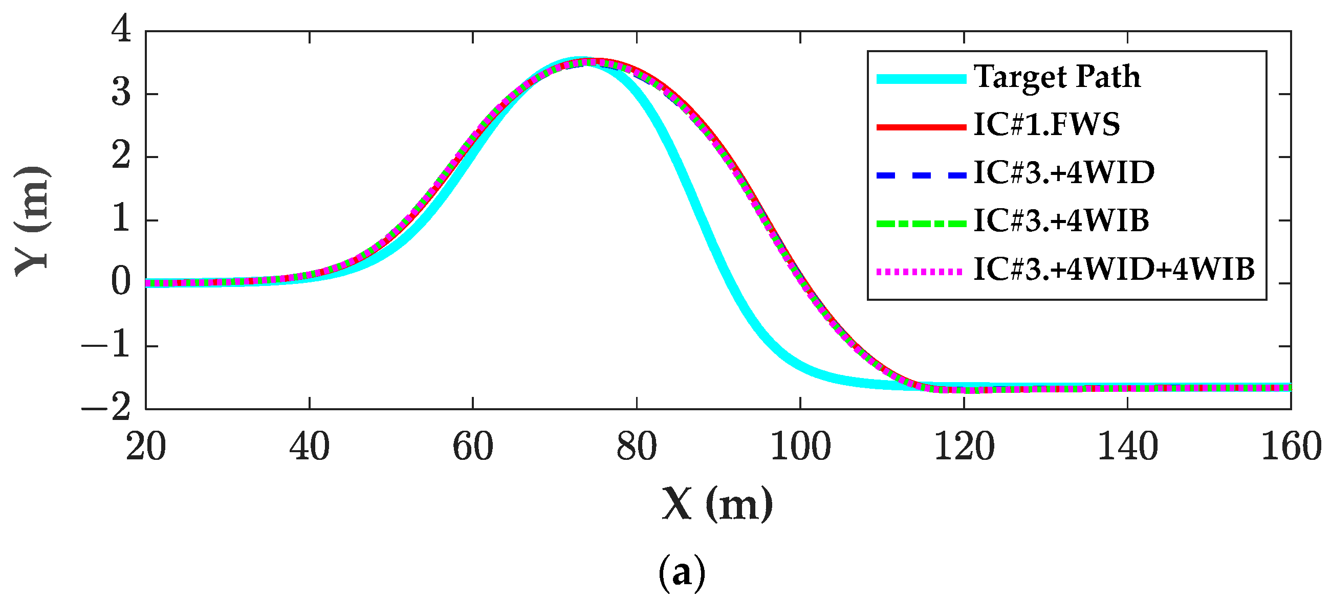
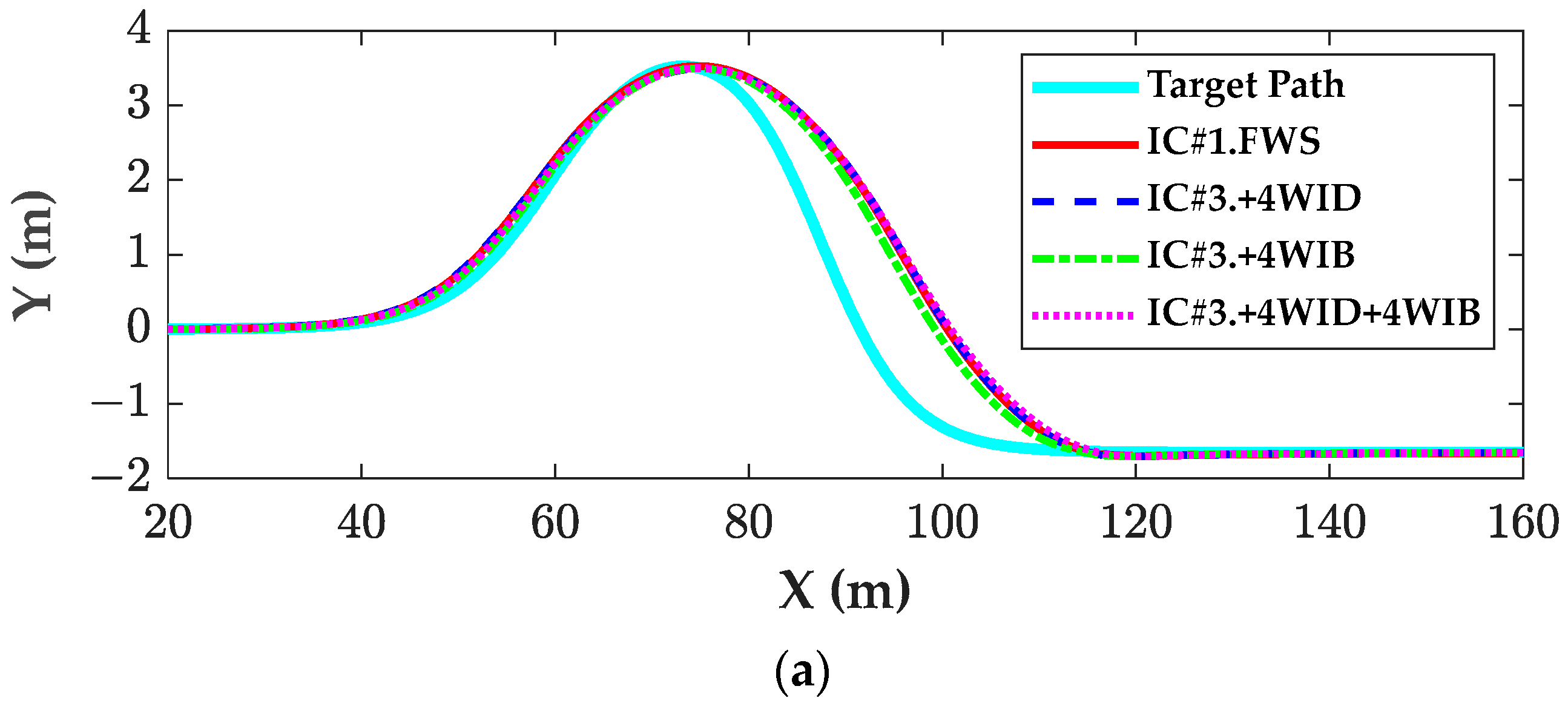
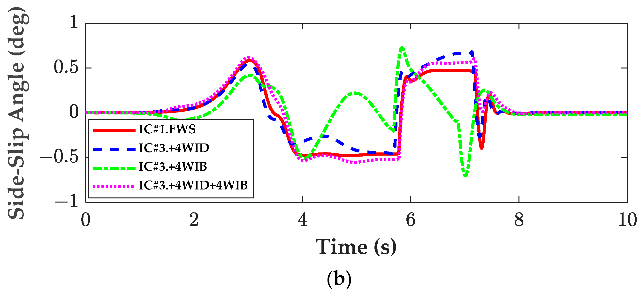
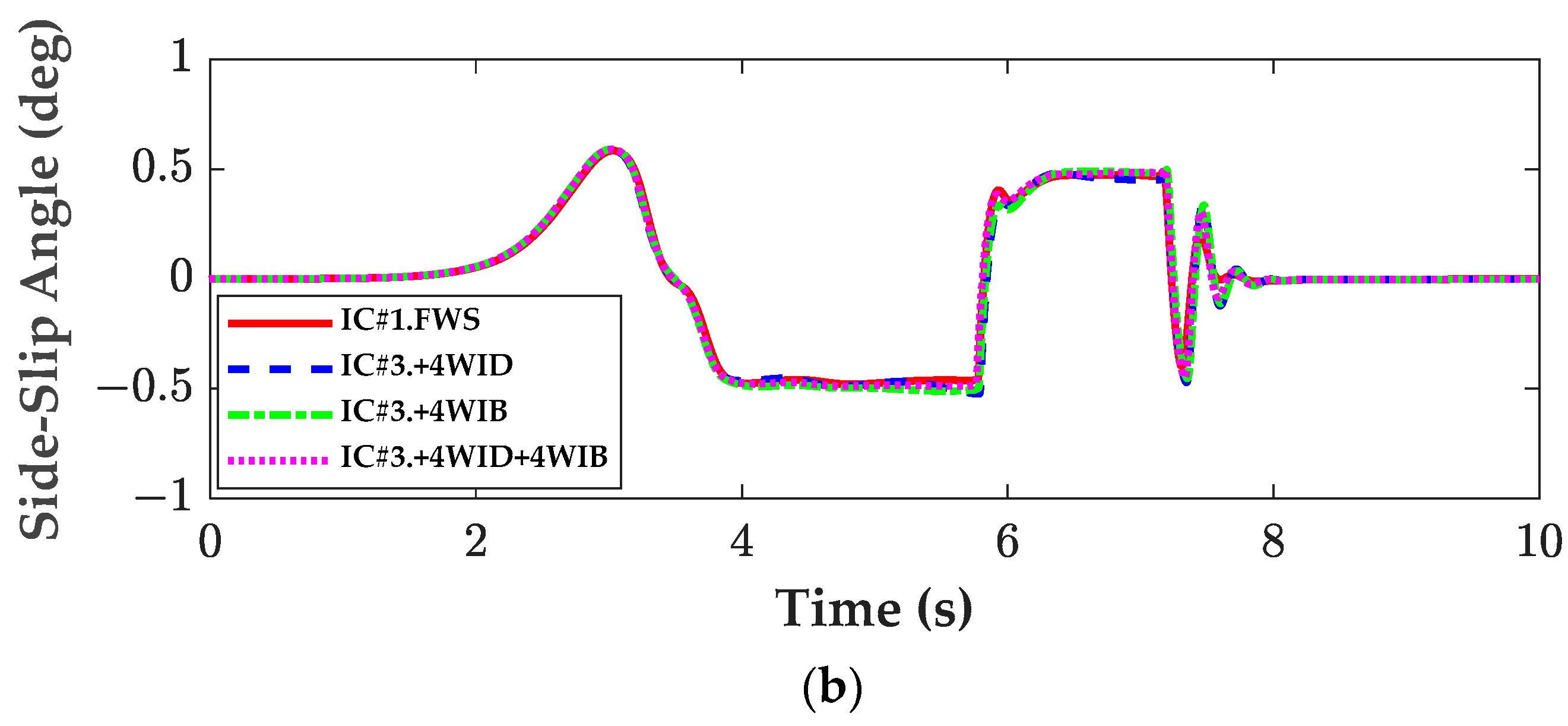
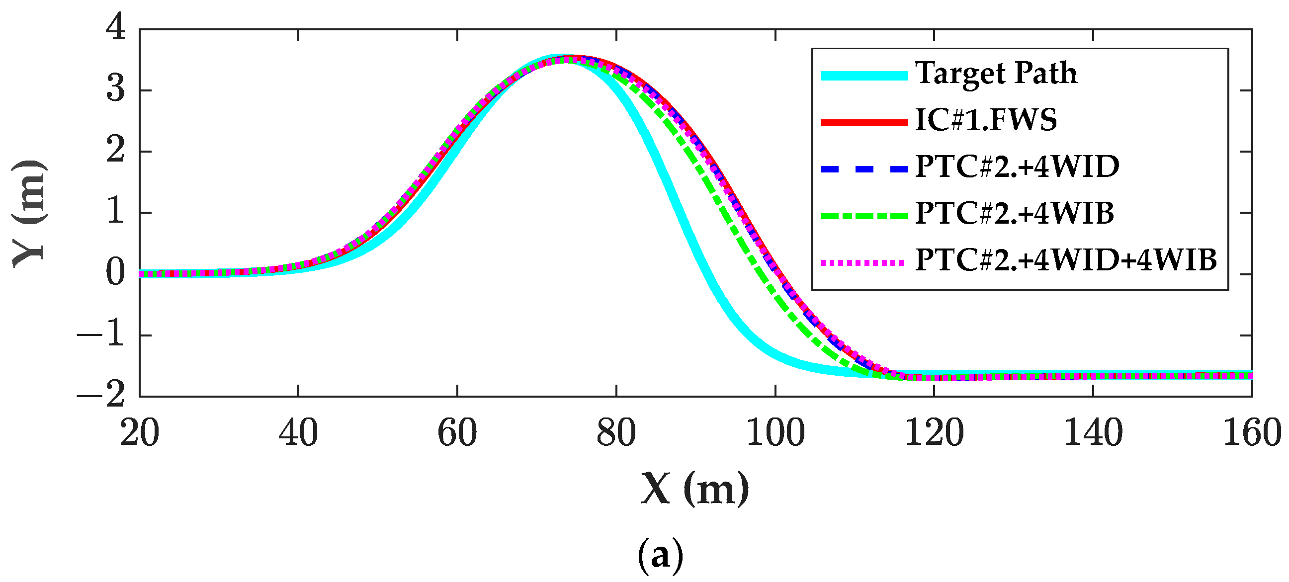
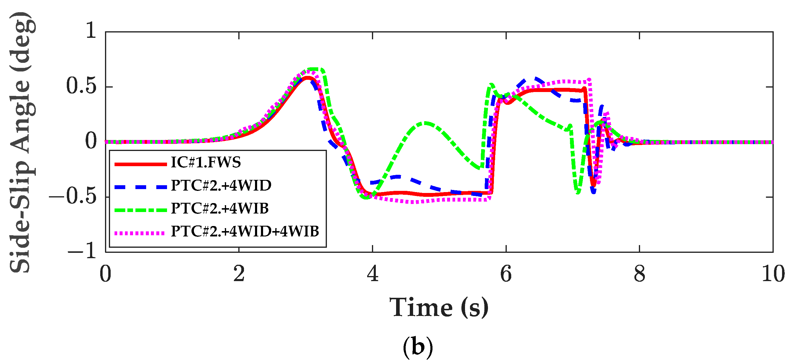
4.3. Simulation with PTC#2 and PTC#3

The second simulation was carried out with PTC#2 and PTC#3. In PTC#2, the front steering angle needed to calculate the reference yaw rate is generated using the IC#1 of PTC#1. This is identical to PTC#3 except the reference yaw rate is calculated from a target path. With the reference yaw rate, ∆M_z is calculated using SMC. For this reason, RWS, 4WID, and 4WIB were used to generate ∆M_z in PTC#2 and PTC#3. Because PTC#2 and PTC#2 use the IC#1 of PTC#1 to generate δ_f, the tuning parameters of PTC#2 and PTC#3 are identical to those of PTC#1.

Table 4. Summary of the simulation results for PTC#2.

Actuator Combinations	∆X (m)	∆Y (m)	OS%	∆DX (m)	∆SX (m)	MASSA (deg)	MASSAR (deg/s)
+4WID	1.50	−0.012	0.9	8.70	4.53	0.58	14.13
+4WIB	0.52	−0.036	0.9	6.66	2.40	0.66	12.56
+4WID + 4WIB	1.15	−0.028	1.0	8.89	5.39	0.64	13.39
+RWS	0.39	0.020	0.9	7.80	4.26	1.84	12.41
+4WID	0.42	0.026	0.9	7.66	3.88	1.67	12.39
+4WIB	0.68	0.023	0.9	8.02	4.24	1.54	12.08
+4WID + 4WIB	0.65	0.015	0.7	8.29	4.88	1.44	11.47

and

Table 5. Summary of the simulation results for PTC#3.

Actuator Combinations	∆X (m)	∆Y (m)	OS%	∆DX (m)	∆SX (m)	MASSA (deg)	MASSAR (deg/s)
+4WID	1.75	−0.033	1.0	9.07	4.76	0.68	13.59
+4WIB	1.56	−0.029	1.0	7.70	4.02	0.73	12.42
+4WID + 4WIB	1.67	−0.024	1.0	9.34	5.70	0.62	12.28
+RWS	1.08	−0.034	1.0	8.41	5.59	1.75	14.35
+4WID	0.93	−0.034	0.9	8.12	4.80	1.59	13.93
+4WIB	1.51	0.004	0.9	9.10	5.82	1.51	13.85
+4WID + 4WIB	1.01	−0.020	1.0	8.60	4.88	1.46	13.80

summarize the simulation results of PTC#2 and PTC#3, respectively.

Table 6. Summary of the best results for PTC#1, PTC#2, and PTC#3.

PTC	Actuator Combinations	∆X (m)	∆Y (m)	OS%	∆DX (m)	∆SX (m)	MASSA (deg)	MASSAR (deg/s)
PTC#1	IC#1: FWS	1.57	0.002	1.0	8.98	4.84	0.58	13.13
	IC#2: RWS	1.61	0.013	0.9	9.12	5.06	1.67	14.73
	IC#3: FWS + RWS	1.25	−0.003	0.9	8.74	4.58	1.36	13.84
	IC#4: FWS + RWS + 4WID	1.45	−0.002	0.9	9.21	5.07	2.09	15.30
PTC#2	FWS + 4WIB	0.52	−0.036	0.9	6.66	2.40	0.66	12.56
	FWS + 4WID	1.5	−0.012	0.9	8.70	4.53	0.58	14.13
PTC#3	FWS + RWS + 4WID	0.93	−0.034	0.9	8.12	4.80	1.59	13.93
	FWS + RWS + 4WIB	1.51	0.004	0.9	9.10	5.82	1.51	13.85

shows the best and worst results for PTC#1, PTC#2, and PTC#3. In Table 5, IC#1 and IC#2 of PTC#1 are selected as a baseline, and the gray rows indicate the worst results.

Table 7. Velocity gains and weights of LQ objective functions for PTC#2.

Actuator Combinations	tp	ξ1	ξ2	ξ3	ξ4	ξ5
+4WID	0.065	0.0539	0.005	0.05	0.50	0.03
+4WIB	0.065	0.0740	0.005	0.05	0.50	0.03
+4WID + 4WIB	0.065	0.0626	0.005	0.05	0.50	0.03
+RWS	0.060	0.0700	0.005	0.10	0.50	0.03
+4WID	0.060	0.0818	0.005	0.10	0.50	0.03
+4WIB	0.060	0.0656	0.005	0.10	0.50	0.03
+4WID + 4WIB	0.060	0.0725	0.005	0.10	0.50	0.03

and

Table 8. Velocity gains and weights of LQ objective functions for PTC#3.

Actuator Combinations	tp	ξ1	ξ2	ξ3	ξ4	ξ5
+4WID	0.07	0.0734	0.010	0.05	0.50	0.03
+4WIB	0.07	0.1172	0.015	0.05	0.50	0.03
+4WID + 4WIB	0.07	0.1123	0.015	0.10	0.50	0.03
+RWS	0.07	0.0969	0.010	0.10	0.50	0.03
+4WID	0.07	0.1012	0.010	0.10	0.50	0.03
+4WIB	0.07	0.0935	0.010	0.10	0.50	0.03
+4WID + 4WIB	0.07	0.1045	0.010	0.10	0.50	0.03

show the velocity gains and weights of LQ objective functions for PTC#2 and PTC#3, which correspond to Table 4 and Table 5, respectively. Figure 8, Figure 9, Figure 10 and Figure 11 show the trajectories and the side-slip angles of each actuator combination of PTC#2 and PTC#3, respectively. As shown in Table 4, the use of RWS increases MASSA, which is identical to PTC#1. Instead, ∆X is significantly reduced by RWS. As shown in Table 5, this tendency can also be identified via PTC#3. Without RWS, the 4WIB of PTC#2 provided the best result among PTC#1, PTC#2, and PTC#3. This fact can be identified in Figure 8. With RWS, the 4WID of PTC#2 provided a good result although MASSA was increased via RWS. By comparing the results among Table 2, Table 4 and Table 6, it can be identified that PTC#2 is superior to PTC#1 in terms of path-tracking performance. By comparing PTC#1 and PTC#3 as shown in Table 1, Table 5 and Table 6, PTC#1 and PTC#3 have no superiority over each other in terms of path-tracking performance.

Although PTC#2 provided better results than PTC#1, there are few differences among PTC#1, PTC#2, and PTC#3, as shown in the trajectories of Figure 5, Figure 6, Figure 7, Figure 8, Figure 9, Figure 10 and Figure 11. The side-slip angles are less than 3° for all controllers, which is acceptable in terms of lateral stability. PTC#1 and PTC#3 require a two-level controller. Especially, IC#1 and IC#2 of PTC#1 do not require any control allocation schemes. On the contrary, PTC#2 requires a three-level controller including a yaw rate tracking controller and control allocation. As shown in Section 2, the yaw rate tracking controller and control allocation require several variables that are difficult to measure. For this reason, IC#1 and IC#2 of PTC#1 are the best choices for designing a path-tracking controller because they are the simplest among the controllers. Moreover, IC#1 of PTC#1 is preferred to IC#2 because it gives a smaller side-slip angle than IC#2.

5. Conclusions

The aim of this study is to compare three types of coordinated controllers, i.e., PTC#1, PTC#2, and PTC#3 on low-friction roads. With the state-space model derived from a 2-DOF bicycle model and a target path, the three controllers were designed. To calculate the steering angles and yaw moment control, LQR was designed. For yaw rate tracking, SMC was designed. As an actuator for path tracking and yaw moment generation, FWS, RWS, 4WS, 4WID, and 4WIB were adopted. For yaw moment distribution or control allocation with the multiple actuators, the WLS-based method was applied. To check the path-tracking performance of each controller, a simulation was carried out using the vehicle simulation package CarSim. For simulation, double lane change for collision avoidance was adopted as a test scenario. From the simulation results, it was shown that PTC#2 is superior to PTC#1 and PTC#3, and that there are little differences among PTC#1 and PTC#3. For this reason, PTC#3 is not recommended as a path-tracking controller. However, there are small differences between PTC#1 and PTC#2 in terms of path-tracking performance except for the peak’s lateral offset and the settling delay. PTC#1 requires a two-level controller and PTC#2 uses a three-level control structure. Moreover, IC#1 and IC#2 of PTC#1 do not require yaw rate tracking and control allocation. As provided in Section 2, the yaw rate tracking controller and control allocation require several variables that are difficult to measure. Because the simplest has been shown to be the best, it is recommended that PTC#1 is the best controller for coordinated control of path tracking and vehicle stability control on low-friction roads. This conclusion was also drawn in the previous research [12]. As pointed out in the previous research, there are no significant differences among actuator combinations [13]. In other words, FWS or 4WS itself is quite enough for coordinated control of path tracking and vehicle stability control. Another conclusion from the simulation results is that it is important to tune the controller gain or select a controller type that is effective on both high- and low-friction roads.

References

1. Montanaro, U.; Dixit, S.; Fallaha, S.; Dianatib, M.; Stevensc, A.; Oxtobyd, D.; Mouzakitisd, A. Towards connected autonomous driving: Review of use-cases. Veh. Syst. Dyn. 2019, 57, 779–814. [Google Scholar] [CrossRef]
2. Yurtsever, E.; Lambert, J.; Carballo, A.; Takeda, K. A survey of autonomous driving: Common practices and emerging technologies. IEEE Access 2020, 8, 58443–58469. [Google Scholar] [CrossRef]
3. Omeiza, D.; Webb, H.; Jirotka, M.; Kunze, M. Explanations in autonomous driving: A survey. IEEE Trans. Intell. Transp. Syst. 2022, 23, 10142–10162. [Google Scholar] [CrossRef]
4. Sorniotti, A.; Barber, P.; De Pinto, S. Path tracking for automated driving: A tutorial on control system formulations and ongoing research. In Automated Driving; Watzenig, D., Horn, M., Eds.; Springer: Cham, Switzerland, 2017. [Google Scholar]
5. Amer, N.H.; Hudha, H.Z.K.; Kadir, Z.A. Modelling and control strategies in path tracking control for autonomous ground vehicles: A review of state of the art and challenges. J. Intell. Robot. Syst. 2017, 86, 225–254. [Google Scholar] [CrossRef]
6. Paden, B.; Cap, M.; Yong, S.Z.; Yershov, D.; Frazzoli, E. A survey of motion planning and control techniques for self-driving urban vehicles. IEEE Trans. Intell. Veh. 2016, 1, 33–55. [Google Scholar] [CrossRef]
7. Bai, G.; Meng, Y.; Liu, L.; Luo, W.; Gu, Q.; Liu, L. Review and comparison of path tracking based on model predictive control. Electronics 2019, 8, 10. [Google Scholar] [CrossRef]
8. Yao, Q.; Tian, Y.; Wang, Q.; Wang, S. Control strategies on path tracking for autonomous vehicle: State of the art and future challenges. IEEE Access 2020, 8, 161211–161222. [Google Scholar] [CrossRef]
9. Rokonuzzaman, M.; Mohajer, N.; Nahavandi, S.; Mohamed, S. Review and performance evaluation of path tracking controllers of autonomous vehicles. IET Intell. Transp. Syst. 2021, 15, 646–670. [Google Scholar] [CrossRef]
10. Stano, P.; Montanaro, U.; Tavernini, D.; Tufo, M.; Fiengo, G.; Novella, L.; Sorniotti, A. Model predictive path tracking control for automated road vehicles: A review. Annu. Rev. Control 2022, 55, 194–236. [Google Scholar] [CrossRef]
11. Jeong, Y.; Yim, S. Integrated path tracking and lateral stability control with four-wheel independent steering for autonomous electric vehicles on low friction roads. Machines 2022, 10, 650. [Google Scholar] [CrossRef]
12. Lee, J.; Yim, S. Comparative study of path tracking controllers on low friction roads for autonomous vehicles. Machines 2023, 11, 403. [Google Scholar] [CrossRef]
13. Park, M.; Yim, S. Comparative study on effects of input configurations of linear quadratic controller on path tracking performance under low friction condition. Actuators 2023, 12, 151. [Google Scholar] [CrossRef]
14. Ahangarnejad, A.H.; Radmehr, A.; Ahmadian, M. A review of vehicle active safety control methods: From antilock brakes to semiautonomy. J. Vib. Control 2021, 27, 1683–1712. [Google Scholar] [CrossRef]
15. Zhang, L.; Zhang, Z.; Wang, Z.; Deng, J.; Dorrell, D.G. Chassis coordinated control for full x-by-wire vehicles—A review. Chin. J. Mech. Eng. 2021, 34, 42. [Google Scholar] [CrossRef]
16. Peng, H.; Chen, X. Active safety control of x-by-wire electric vehicles: A survey. SAE Int. J. Veh. Dyn. Stab. NVH 2022, 6, 115–133. [Google Scholar] [CrossRef]
17. Indu, K.; Kumar, M.A. Electric vehicle control and driving safety systems: A review. IETE J. Res. 2023, 6, 482–498. [Google Scholar] [CrossRef]
18. Yim, S. Comparison among active front, front independent, 4-wheel and 4-wheel independent steering systems for vehicle stability control. Electronics 2020, 9, 798. [Google Scholar] [CrossRef]
19. Nah, J.; Yim, S. Vehicle stability control with four-wheel independent braking, drive and steering on in-wheel motor-driven electric vehicles. Electronics 2020, 9, 1934. [Google Scholar] [CrossRef]
20. Hang, P.; Chen, X.; Luo, F. Path-Tracking Controller Design for a 4WIS and 4WID Electric Vehicle with Steer-by-Wire System (No. 2017-01-1954); SAE Technical Paper: Warrendale, PA, USA, 2017. [Google Scholar]
21. Guo, J.; Luo, Y.; Li, K. An adaptive hierarchical trajectory following control approach of autonomous four-wheel independent drive electric vehicles. IEEE Trans. Intell. Transp. Syst. 2018, 19, 2482–2492. [Google Scholar] [CrossRef]
22. Guo, J.; Luo, Y.; Li, K.; Dai, Y. Coordinated path-following and direct yaw-moment control of autonomous electric vehicles with sideslip angle estimation. Mech. Syst. Signal Process. 2018, 105, 183–199. [Google Scholar] [CrossRef]
23. Hang, P.; Chen, X.; Luo, F. LPV/H controller design for path tracking of autonomous ground vehicles through four-wheel steering and direct yaw-moment control. Int. J. Automot. Technol. 2019, 20, 679–691. [Google Scholar] [CrossRef]
24. Peng, H.; Wang, W.; An, Q.; Xiang, C.; Li, L. Path tracking and direct yaw moment coordinated control based on robust MPC with the finite time horizon for autonomous independent-drive vehicles. IEEE Trans. Veh. Technol. 2020, 69, 6053–6066. [Google Scholar] [CrossRef]
25. Wang, Y.; Shao, Q.; Zhou, J.; Zheng, H.; Chen, H. Longitudinal and lateral control of autonomous vehicles in multi-vehicle driving environments. IET Intell. Transp. Syst. 2020, 14, 924–935. [Google Scholar] [CrossRef]
26. Wu, H.; Li, Z.; Si, Z. Trajectory tracking control for four-wheel independent drive intelligent vehicle based on model predictive control and sliding mode control. Adv. Mech. Eng. 2021, 13, 16878140211045142. [Google Scholar] [CrossRef]
27. Xiang, C.; Peng, H.; Wang, W.; Li, L.; An, Q.; Cheng, S. Path tracking coordinated control strategy for autonomous four in-wheel-motor independent-drive vehicles with consideration of lateral stability. Proc. Inst. Mech. Eng. Part D J. Automob. Eng. 2021, 235, 1023–1036. [Google Scholar] [CrossRef]
28. Barari, A.; Afshari, S.S.; Liang, X. Coordinated control for path-following of an autonomous four in-wheel motor drive electric vehicle. Proc. Inst. Mech. Eng. Part C J. Mech. Eng. Sci. 2022, 236, 6335–6346. [Google Scholar] [CrossRef]
29. Wang, W.; Zhang, Y.; Yang, C.; Qie, T.; Ma, M. Adaptive model predictive control-based path following control for four-wheel independent drive automated vehicles. IEEE Trans. Intell. Transp. Syst. 2022, 23, 14399–14412. [Google Scholar] [CrossRef]
30. Jin, L.; Gao, L.; Jiang, Y.; Chen, M.; Zheng, Y.; Li, K. Research on the control and coordination of four-wheel independent driving/steering electric vehicle. Adv. Mech. Eng. 2017, 9, 1687814017698877. [Google Scholar] [CrossRef]
31. Ren, Y.; Zheng, L.; Khajepour, A. Integrated model predictive and torque vectoring control for path tracking of 4-wheeldriven autonomous vehicles. IET Intell. Transp. Syst. 2019, 13, 98–107. [Google Scholar] [CrossRef]
32. Guo, L.; Ge, P.; Yue, M.; Li, J. Trajectory tracking algorithm in a hierarchical strategy for electric vehicle driven by four independent in-wheel motors. J. Chin. Inst. Eng. 2020, 43, 807–818. [Google Scholar] [CrossRef]
33. Ahn, T.; Lee, Y.; Park, K. Design of integrated autonomous driving control system that incorporates chassis controllers for improving path tracking performance and vehicle stability. Electronics 2021, 10, 144. [Google Scholar] [CrossRef]
34. Liang, Y.; Li, Y.; Zheng, L.; Yu, Y.; Ren, Y. Yaw rate tracking-based path-following control for four-wheel independent driving and four-wheel independent steering autonomous vehicles considering the coordination with dynamics stability. Proc. Inst. Mech. Eng. Part D J. Automob. Eng. 2021, 235, 260–272. [Google Scholar] [CrossRef]
35. Xie, J.; Xu, X.; Wang, F.; Tang, Z.; Chen, L. Coordinated control based path following of distributed drive autonomous electric vehicles with yaw-moment control. Control Eng. Pract. 2021, 106, 104659. [Google Scholar] [CrossRef]
36. Tong, Y.; Jing, H.; Kuang, B.; Wang, G.; Liu, F.; Yang, Z. Trajectory tracking control for four-wheel independently driven electric vehicle based on model predictive control and sliding model control. In Proceedings of the 2021 5th CAA International Conference on Vehicular Control and Intelligence (CVCI), Tianjin, China, 29–31 October 2021. [Google Scholar]
37. Du, Q.; Zhu, C.; Li, Q.; Tian, B.; Li, L. Optimal path tracking control for intelligent four-wheel steering vehicles based on MPC and state estimation. Proc. Inst. Mech. Eng. Part D J. Automob. Eng. 2022, 236, 1964–1976. [Google Scholar] [CrossRef]
38. Sun, X.; Wang, Y.; Hu, W.; Cai, Y.; Huang, C.; Chen, L. Path tracking control strategy for the intelligent vehicle considering tire nonlinear cornering characteristics in the PWA form. J. Frankl. Inst. 2022, 359, 2487–2513. [Google Scholar] [CrossRef]
39. Jeong, Y.; Yim, S. Path tracking control with four-wheel independent steering, driving and braking systems for autonomous electric vehicles. IEEE Access 2022, 10, 74733–74746. [Google Scholar] [CrossRef]
40. Hu, H.; Bei, S.; Zhao, Q.; Han, X.; Zhou, D.; Zhou, X.; Li, B. Research on trajectory tracking of sliding mode control based on adaptive preview time. Actuators 2022, 11, 34. [Google Scholar] [CrossRef]
41. Tarhini, F.; Talj, R.; Doumiati, M. Adaptive look-ahead distance based on an intelligent fuzzy decision for an autonomous vehicle. In Proceedings of the 2023 IEEE Intelligent Vehicles Symposium (IV), Anchorage, AK, USA, 4–7 June 2023. [Google Scholar]
42. Wong, H.Y. Theory of Ground Vehicles, 3rd ed.; John Wiley and Sons, Inc.: New York, NY, USA, 2001. [Google Scholar]
43. Rajamani, R. Vehicle Dynamics and Control; Springer: New York, NY, USA, 2006. [Google Scholar]
44. Bryson, A.E.; Ho, Y.C. Applied Optimal Control; Hemisphere: New York, NY, USA, 1975. [Google Scholar]
45. Wang, J.; Wang, R.; Jing, H.; Chen, N. Coordinated active steering and four-wheel independently driving/braking control with control allocation. Asian J. Control 2016, 18, 98–111. [Google Scholar] [CrossRef]
46. Rezaeian, A.; Zarringhalam, R.; Fallah, S.; Melek, W.; Khajepour, A.; Chen, S.-K.; Moshchuck, N.; Litkouhi, B. Novel tire force estimation strategy for real-time implementation on vehicle applications. IEEE Trans. Veh. Technol. 2015, 64, 2231–2241. [Google Scholar] [CrossRef]
47. Yim, S.; Choi, J.; Yi, K. Coordinated control of hybrid 4WD vehicles for enhanced maneuverability and lateral stability. IEEE Trans. Veh. Technol. 2012, 61, 1946–1950. [Google Scholar] [CrossRef]
48. Yim, S. Coordinated control with electronic stability control and active steering devices. J. Mech. Sci. Technol. 2015, 29, 5409–5416. [Google Scholar] [CrossRef]
49. Yakub, F.; Mori, Y. Comparative study of autonomous path-following vehicle control via model predictive control and linear quadratic control. Proc. Inst. Mech. Eng. Part D J Automob. Eng. 2015, 229, 1695–1714. [Google Scholar] [CrossRef]
50. Kim, H.H.; Ryu, J. Sideslip angle estimation considering short-duration longitudinal velocity variation. Int. J. Automot. Technol. 2011, 12, 545–553. [Google Scholar] [CrossRef]
51. National Highway Traffic Safety Administration. FMVSS No. 126, Electronic Stability Control Systems: NHTSA Final Regulatory Impact Analysis; National Highway Traffic Safety Administration: Washington, DC, USA, 2007. [Google Scholar]
52. Mechanical Simulation Corporation. VS Browser: Reference Manual, The Graphical User Interfaces of BikeSim, CarSim, and TruckSim; Mechanical Simulation Corporation: Ann Arbor, MI, USA, 2009. [Google Scholar]
Figure 1. Structures of PTC#1, PTC#2, and PTC#3.
Actuators 12 00398 g001
Figure 2. Coordinates and variables of the 2-DOF bicycle model and the target path.
Actuators 12 00398 g002
Figure 3. Coordinate system on vehicle geometry with tire forces and yaw moment control.
Actuators 12 00398 g003
Figure 4. Measures for path-tracking performance.
Actuators 12 00398 g004
Figure 5. Simulation results with IC#1 and IC#3 of PTC#1. (a) Trajectories. (b) Side-slip angles.
Actuators 12 00398 g005aActuators 12 00398 g005b
Figure 6. Simulation results with IC#2 and IC#3 of PTC#1. (a) Trajectories. (b) Side-slip angles.
Actuators 12 00398 g006
Figure 7. Simulation results with IC#2 and IC#4 of PTC#1. (a) Trajectories. (b) Side-slip angles.
Actuators 12 00398 g007aActuators 12 00398 g007b
Figure 8. Simulation results with IC#1 and PTC#2. (a) Trajectories. (b) Side-slip angles.
Actuators 12 00398 g008aActuators 12 00398 g008b
Figure 9. Simulation results with IC#2 and PTC#2. (a) Trajectories. (b) Side-slip angles.
Actuators 12 00398 g009
Figure 10. Simulation results with IC#1 and PTC#3. (a) Trajectories. (b) Side-slip angles.
Actuators 12 00398 g010aActuators 12 00398 g010b
Figure 11. Simulation results with IC#2 and PTC#3. (a) Trajectories. (b) Side-slip angles.
Actuators 12 00398 g011