Sensor Fault Diagnosis, Isolation, and Accommodation for Heating, Ventilating, and Air Conditioning Systems Based on Soft Sensor

Abstract

Heating, Ventilating, and Air Conditioning (HVAC) systems often suffer from unscheduled maintenance or abnormal shutdown due to the fault of their interior sensor system. Traditional fault diagnosis methods for HVAC sensor systems primarily focus on sensor fault diagnosis and isolation, lacking fault accommodation. Therefore, to realize effective sensor fault detection, identification, and accommodation (SFDIA), a method for HVAC SFDIA based on the soft sensor is proposed. First, a diagnosis soft sensor with multi-variable input is constructed to estimate the output of the physical sensor being diagnosed. The residual between the estimated value of the diagnosis soft sensor and the measurement of the physical sensor is used as an indicator of the sensor’s condition. If the residual exceeds the fault threshold, the sensor is diagnosed to be faulty. In order to maintain valid sensor output, an accommodation soft sensor is constructed using the historical normal value. The erroneous output of the faulty sensor is substituted by the estimated value from the accommodation soft sensor, thereby realizing sensor fault tolerance control. Experimental results demonstrate that the average false alarm rate for sensor fault diagnosis is 1.57% and the average fault diagnosis rate is 96.51%. The predictive mean absolute error (MAE) and root-mean-square error (RMSE) of the recovered soft sensors are 0.0525 and 0.0738, respectively. Thus, the soft sensors developed in this paper exhibit satisfying ability in HVAC SFDIA.

1. Introduction

Sensors serve as “the eyes and ears” of the HVAC control system, monitoring critical variables and providing data support for the control system actuator to make decisions and optimize control. The malfunctioning of sensors can have a negative impact on the system’s functionality, leading to a decrease in overall performance. A reliable sensor system plays a crucial role in risk management strategies to enhance safety and reliability. Specifically, sensor fault detection involves three aspects: (1) detection (determining whether any sensors have experienced faults); (2) isolation (identifying the faulty sensors); and (3) accommodation (replacing faulty data with approximate correct data transmitted to downstream systems) [1]. Therefore, establishing an effective HVAC sensor fault detection, identification, and accommodation (SFDIA) scheme is of significant importance for the long-term stable operation of sensors.

Currently, there is limited research on HVAC SFDIA. Most of the existing research focuses on sensor fault diagnosis and isolation, with a lack of fault compensation. With the advancement of data processing technologies [2], data-driven fault diagnosis methods have gained widespread application. Among them, statistical analysis methods [3,4,5] and artificial intelligence (AI) methods [6,7,8] are highly favored. Principal Component Analysis (PCA) is commonly employed in statistical analysis, yet it struggles with non-linear issues. Its variant, Kernel PCA (KPCA) [9,10], can address non-linear problems, but its computations are complex and unsuitable for large-scale industrial processes [11]. Artificial intelligence methods [12,13] can automatically extract and integrate crucial information from complex data, which is more suitable for nonlinear systems, so it is applied in the field of sensor fault diagnosis [14,15,16]. The above research focuses on fault diagnosis and isolation. Moreover, AI-based classification models require significant amounts of labeled historical fault data, which are often lacking in industrial databases [17,18]. AI-based prediction models often utilize the maximum prediction residual as the fault threshold, without quantitatively evaluating the performance of the fault threshold. Therefore, there is a need for an approach that can realize SFDIA using fault-free data, as well as a quantifiable metric to evaluate fault thresholds. As a combination of mathematical models, data processing, and software technology methods, the soft sensor employs fault-free data to generate a virtual measurement to replace a real sensor measurement realizing SFDIA.

A soft sensor [19,20] is an estimation method based on available physical sensors and process parameters to derive the interested physical variables [21,22]. There are primarily three types of soft sensor models: mechanism-based, knowledge-based, and data-driven methods [23]. However, due to the increasing complexity of industrial processes, soft sensor models based on data-driven approaches are gaining popularity, especially when the necessary prior knowledge is lacking or modeling processes are complex. Chun et al. [24] proposed a data-driven dynamic soft measurement method based on Supervised Bidirectional Long Short-Term Memory to extract and utilize nonlinear dynamic latent information. Ding et al. [25] introduced a deep learning-based modeling framework to develop soft sensor models that are robust to sensor faults, which exhibit a strong resilience to sensor faults and high recovery capability for sensor fault signals. Darvishi et al. [26] established a series of neural network estimators and classifiers, where estimators correspond to virtual sensors for all unreliable sensors, used to replace isolated faulty sensors within the system. Classifiers are employed for detection and isolation tasks, utilizing estimators to reconstruct faulty sensor data. Giovanni et al. [27] developed three kinds of soft sensors such as temperature, airflow, and fan speed by employing linear regression models, statistical models, and non-linear regression models. And a sensor fault diagnosis method using three sensors to mutually corroborate each other is proposed, which has high reliability. Hence, utilizing soft sensors to estimate the faulty physical sensor can not only realize sensor fault diagnosis but also reconstruct the fault data.

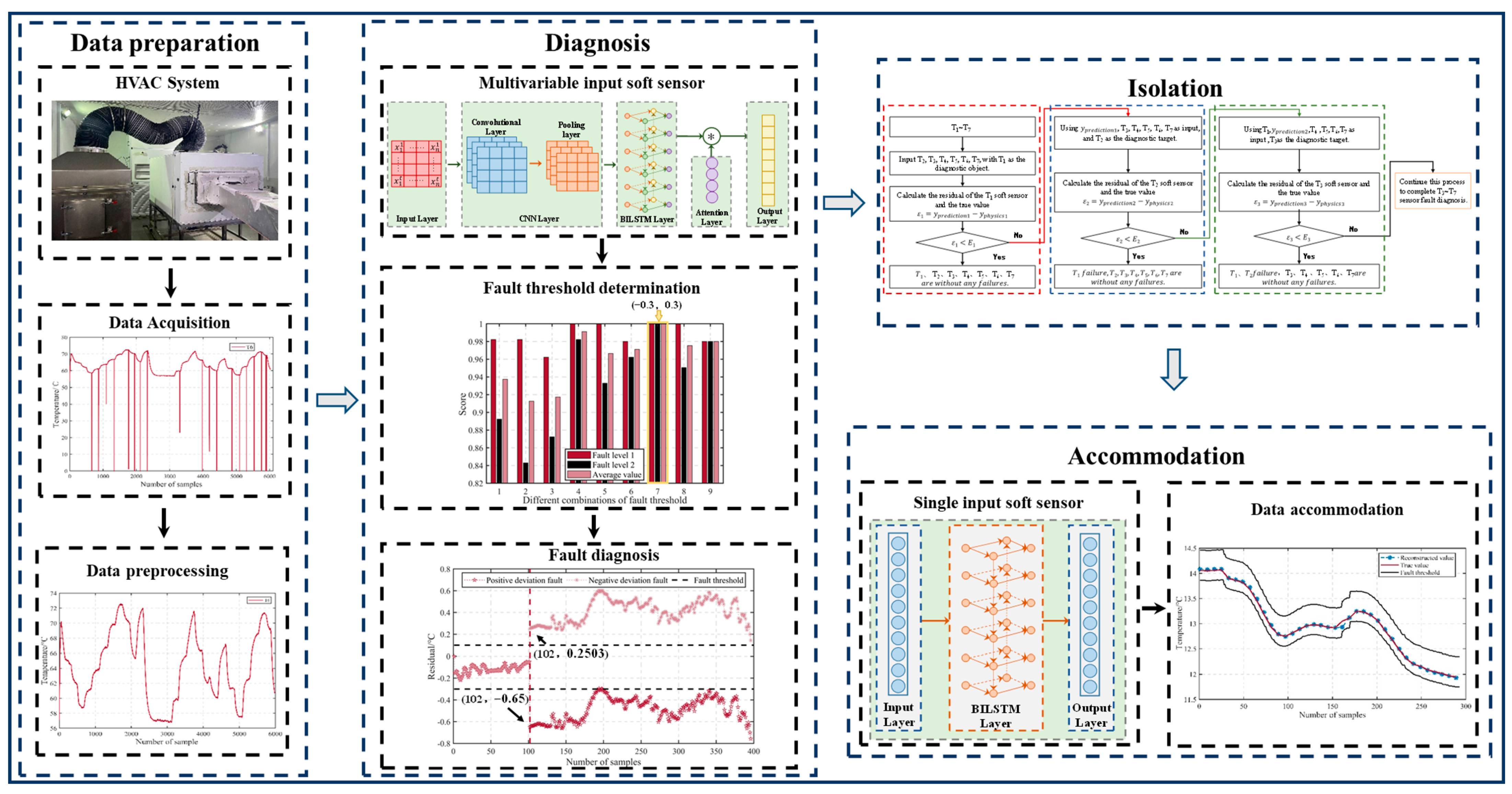
The soft-sensor-based HVAC SFDIA framework, which considers only one sensor fault at a time, consists of three parts. The first part is fault diagnosis. A soft sensor model combining the convolutional neural network, long-short-term memory neural network, and attention mechanism (CNN-BILTM-ATTENTION) is constructed using multidimensional sensor data excluding the diagnosed sensor to estimate the output of the diagnosed sensor. The residual between the estimated and measured value of the diagnosed sensor is calculated. If the residual exceeds the fault threshold, it is considered that the diagnosed sensor is faulty or the input sensor is faulty. The method for determining the fault threshold involves three steps. Firstly, several appropriate fault threshold combinations are identified based on the maximum residual. Subsequently, fault diagnosis test experiments are performed on data containing faults. Finally, the combination with the largest difference between FDR and FAR is chosen as the optimal fault threshold. The second part is fault isolation. Assuming the diagnosed sensor fault, the estimated value of the diagnosed sensor is used instead of the faulty value to estimate and diagnose the second sensor. If the second sensor is normal, it indicates that the diagnosed sensor is faulty. If the second sensor is faulty, the estimated value of the second sensor is used instead of it. The method is repeated to diagnose all input sensors. The third part is fault compensation. A univariate input BILSTM soft sensor model is built using normal data and historical data from before the sensor failure to estimate the sensor’s output and realize the recovery of fault data.

In summary, to realize HVAC sensor fault diagnosis, isolation, and accommodation, a soft-sensor-based method is proposed. The main contributions are as follows:

(1) Establishing an HVAC SFDIA scheme based on the soft sensor, which can realize fault sensor diagnosis, isolation, and fault data recovery.

(2) By utilizing the soft sensor to estimate the diagnosed sensor, the residual between the estimated and sensor measured value is computed and compared with a predetermined threshold. If the residual surpasses the threshold, the estimated value is used to replace the faulty sensor’s measurement, thus realizing the goals of sensor fault diagnosis, isolation, and accommodation.

(3) An evaluation metric for determining the fault threshold is proposed, avoiding the influence of subjective factors and enabling enhanced fault diagnosis effectiveness.

2. Basis of Soft-Sensor-Based HVAC SFDIA

A typical HVAC SFDIA procedure involves three parts.

(1) Diagnosis: utilize historical data to determine whether there has been a sensor malfunction at the current moment.

(2) Isolation: if there is a malfunctioning sensor, identify the faulty sensor’s location.

(3) Accommodation: Determine the first fault data point of the faulty sensor, which is the starting point for data recovery. Use historical normal data before the point to evaluate the correct output value of faulty sensor, ensuring the short-term normal operation of the HVAC system.

2.1. SFDIA Scheme Process Based on Soft Sensor

The soft-sensor-based HVAC SFDIA process is divided into 6 steps, as shown in Figure 1.

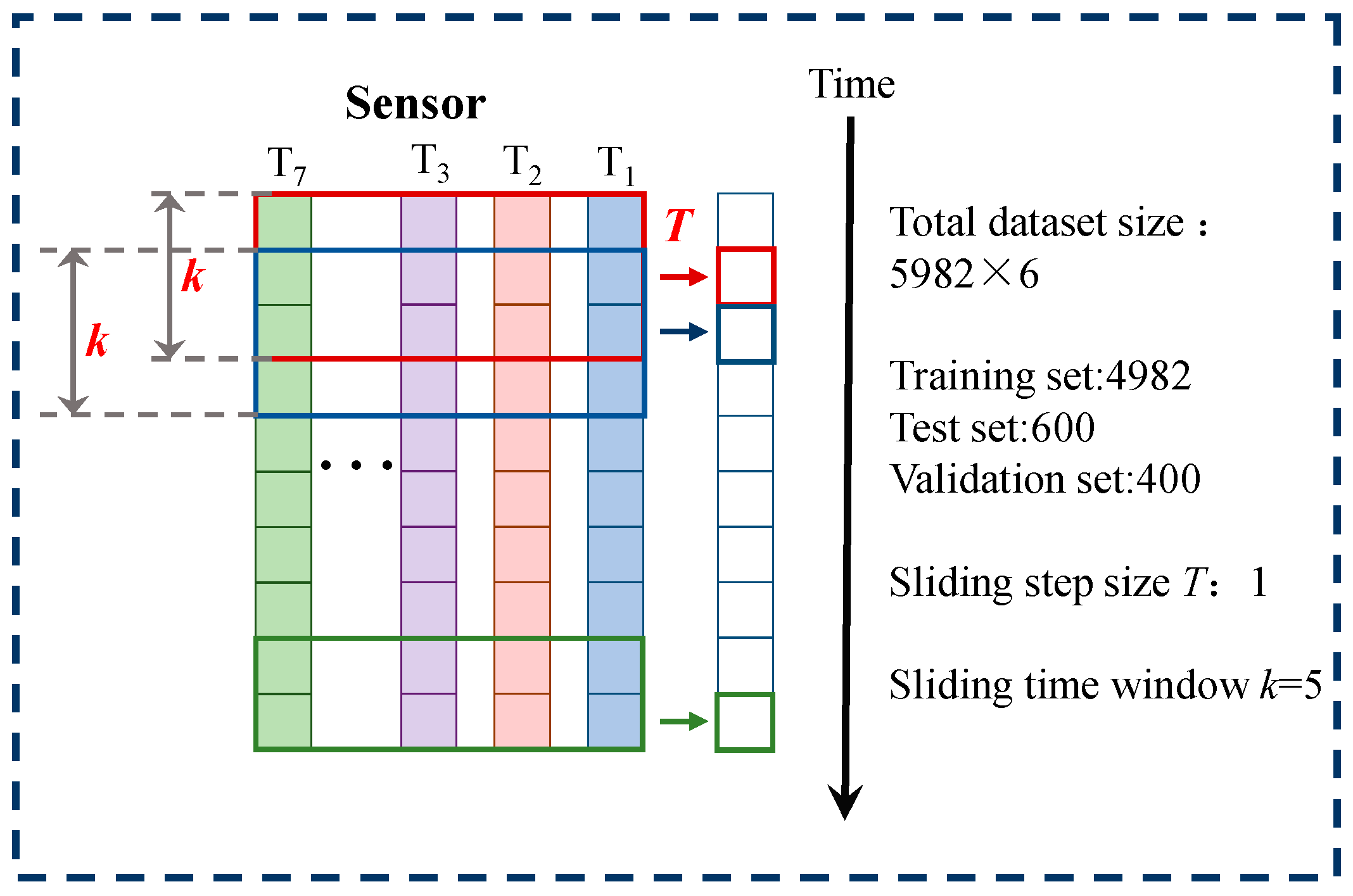
Step 1: Data preprocessing. The experimental data contain unstable data during the startup phase and a few missing data points. A one-dimensional interpolation method is used to fill in missing data. And the unstable data are removed. Subsequently, the data are normalized to eliminate the interference caused by different units of measurement. The data input and time series transformation are illustrated in Figure 2. The training set is used to construct the diagnosis soft sensor for fault diagnosis, the test set is used to determine the optimal combination of fault thresholds, and the validation set is used for fault diagnosis experiments.

Step 2: Constructing a diagnosis soft sensor. Utilize the diagnosed sensor as the label and the other sensors as model inputs. The model uses RMSE as the loss function and Adam optimizer. Additionally, early stopping is added to prevent overfitting of the network.

Step 3: Determining the fault threshold. Calculate the residual sequences between the soft sensor and the physical sensor outputs on the test set to determine the range of fault thresholds. Utilize the score metric from Section 3.2 to select the optimal combination of fault thresholds within the determined range.

Step 4: Fault diagnosis. The trained soft sensor is used to predict the diagnosed sensor. The residual between the predicted value and the measurement is calculated and compared with the fault threshold to determine whether the diagnosed sensor has a fault. When the residuals of five consecutive soft sensor data points exceed the fault threshold, it is considered that a fault has occurred at that data position. In addition, the initial fault data point can be identified. Fault accommodation will start from the point.

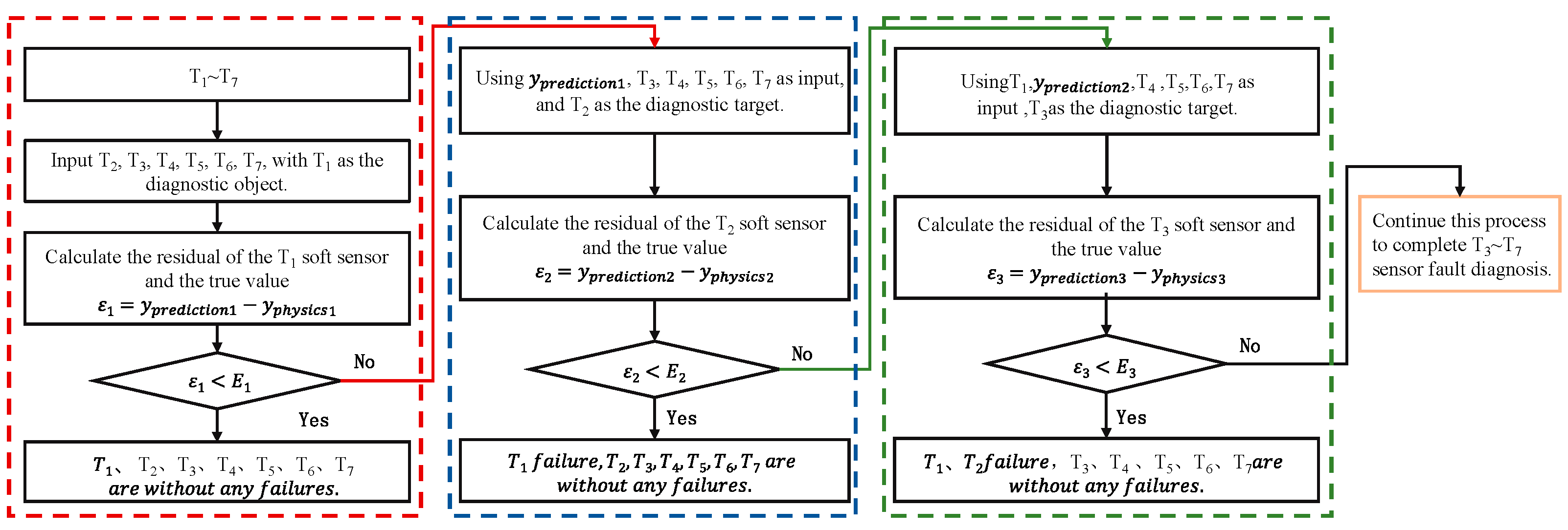
Step 5: Fault isolation. To identify the location of the faulty sensor, repeat steps 2–4 for each sensor individually. Figure 3 shows a subgraph of the fault isolation portion of Figure 1, illustrating the process of clearly identifying faulty sensors. More specifically, first, the T₁ sensor is taken as the diagnostic target. Input T₂~T₇ measurement y_physics2~y_physics7 into the T₁ soft sensor to predict the output of T₁. If the residual ε₁ between the predicted data and the measurement is less than the fault threshold, all sensors are considered normal. Otherwise, it is considered possible that there may be a failure of the T₁ sensor or the input sensor. Assuming a fault in the T₁ sensor, replace the T₁ measurement y_physics1 with the predicted data y_prediction1. Input y_prediction1 and y_physics3~y_physics7 into the T₂ soft sensor to calculate the residual ε₂. If ε₂ is less than the fault threshold, the assumption is true, which indicates a fault in the T₁ sensor while others are normal. Otherwise, if ε₂ exceeds the threshold, the assumption is false, which indicates that the T₁ sensor is normal while a faulty sensor exists in T₂~T₇. Assuming a fault in the T₂ sensor, replace y_physics2 with y_prediction2. Continue diagnosing T₃. Repeat this process to isolate a fault in T₁~T₇ sensors.

Step 6: Fault accommodation. Utilizing the normal data from the faulty sensor as input to train the soft sensor data recovery model, the output values are used as reconstructed data to recover the faulty data.

2.2. Soft Sensor Construction

Soft sensors, as a core component within the SFDIA scheme, plays a crucial role in estimating sensor data. The estimated value is employed to accomplish diagnosis, isolation, and accommodation processes.

The main difference between diagnosis and accommodation soft sensors lies in the external input. Therefore, the design of their internal core models also differs. Considering the time-varying nature of sensor data, both soft sensors need to effectively store the temporal information of input signals. Additionally, diagnosis soft sensors deal with complex multidimensional data that exhibit strong coupling, requiring feature extraction of input information. To help the network capture crucial information while handling complex data, an attention mechanism is introduced to use weighted operation to enable the network to focus on information highly relevant to the task.

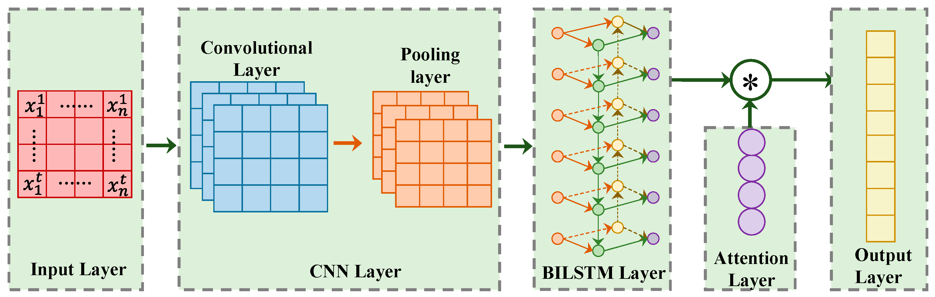
The structure of the CNN-BILSTM-ATTENTION diagnosis soft sensor is depicted in Figure 4, primarily composed of the input layer, CNN layer, BILSTM layer, attention layer, and output layer. Each layer is described as follows:

Input layer: The input layer receives the time-serialized data and feeds them into the convolutional layer, defining the input size. A single data point is represented as Equations (1) and (2):

$$X_1=\left[\begin{array}{cccccc}{x}_1^1& x_2^1& \cdots & x_n^t& \cdots & x_6^1\\ x_1^2& x_2^2& \cdots & x_n^t& \cdots & x_6^2\\ ⋮& ⋮& \cdots & x_n^t& \cdots & \cdots \\ x_1^5& x_2^5& \cdots & x_n^t& \cdots & x_6^5\end{array}\right]$$

(1)

$$Y_1=\left[x_7^5\right]$$

(2)

where $x_n^t$ represents the nth sensor sampled at time t.

CNN layer: This mainly consists of the convolutional layer and pooling layer. The convolutional layer performs sliding convolutions of the multidimensional input signals along the time sequence to achieve feature extraction. The calculation process is shown in (3) and (4).

$$x_j^l=f\left(\sum _{i=1}^N{x}_i^{l-1}\ast k_{ij}^l+b_j^l\right)$$

(3)

$$A^{\left[l\right]}=\max \{0,x_j^l\}$$

(4)

where $x_j^l$ represents the jth feature output of the lth layer, f(·) is the activation function, N is the number of input signals, * denotes the convolution operator, $k_{ij}^l$ is the convolution kernel, $b_j^l$ is the bias term, and $A^{\left[l\right]}$ is the output of the activation function. The ReLU activation function is used to perform a non-linear transformation on the output.

The pooling layer utilizes downsampling to merge highly similar features, reducing spatial dimensions, lowering computational complexity, while preserving feature invariance and locality. The max-pooling operation is adopted, and the calculation formula is shown as (5).

$${Pl}^{\left[l\right]}=\max \left\{A^{\left[l\right]}\right\}$$

(5)

where Pl^[l] represents the output of the pooling layer.

BILSTM layer: Adjacent sensor data often exhibit strong correlations. Data at any time point are highly correlated with the data at its neighboring time points. The BILSTM network consists of two LSTM networks in opposite directions, providing more comprehensive information for each time point. The calculation formula is as follows:

$$\left\{\begin{array}{c}\overrightarrow{h_t}={\displaystyle \stackrel{⃑}{LSTM}}\left(h_{t-1},x_t,C_{t-1}\right) t\in \left[1,T\right]\\ \overleftarrow{h_t}={\displaystyle \stackrel{⃐}{LSTM}}\left(h_{t+1},x_t,C_{t+1}\right) t\in \left[T,1\right]\\ H_t=\left[\overrightarrow{h_t},\overleftarrow{h_t}\right]\end{array}\right.$$

(6)

where H_t represents the total output of the hidden layer at time t, $\overrightarrow{h_t}$ is the forward output of the LSTM hidden layer at time t, $\overleftarrow{h_t}$ is the backward output of the LSTM hidden layer at time t, h_t is the output of the hidden layer at time t, C_t is the state value of the LSTM hidden layer’s state unit, and x_t is the input of the model at time t.

Attention layer: The attention mechanism is employed to weight the output vectors of the BILSTM network and perform a weighted sum. The softmax function is used to assign different weights to the outputs at different time steps, aiming to maximize the extraction of temporal feature information and achieve better evaluation results.

$$\mathrm{A}\mathrm{t}\mathrm{t}\mathrm{e}\mathrm{n}\mathrm{t}\mathrm{i}\mathrm{o}\mathrm{n}\left(\mathrm{Q},\mathrm{K},\mathrm{V}\right)=\mathrm{S}\mathrm{o}\mathrm{f}\mathrm{t}\mathrm{m}\mathrm{a}\mathrm{x}\left(\frac{Q{K}^T}{\sqrt{d_k}}\right)\mathrm{V}$$

(7)

$$\left\{\begin{array}{c}Q=W_{Q}X\\ K=W_{K}X\\ V=W_{V}X\end{array}\right.$$

(8)

where Q, K, and V represent the query matrix, key matrix, and value matrix, respectively. W_Q, W_K, and W_V are weight matrices, and d_k represents the vector dimension of Q.

Output layer: a fully connected layer is used with the ReLU activation function to generate a single evaluated value.

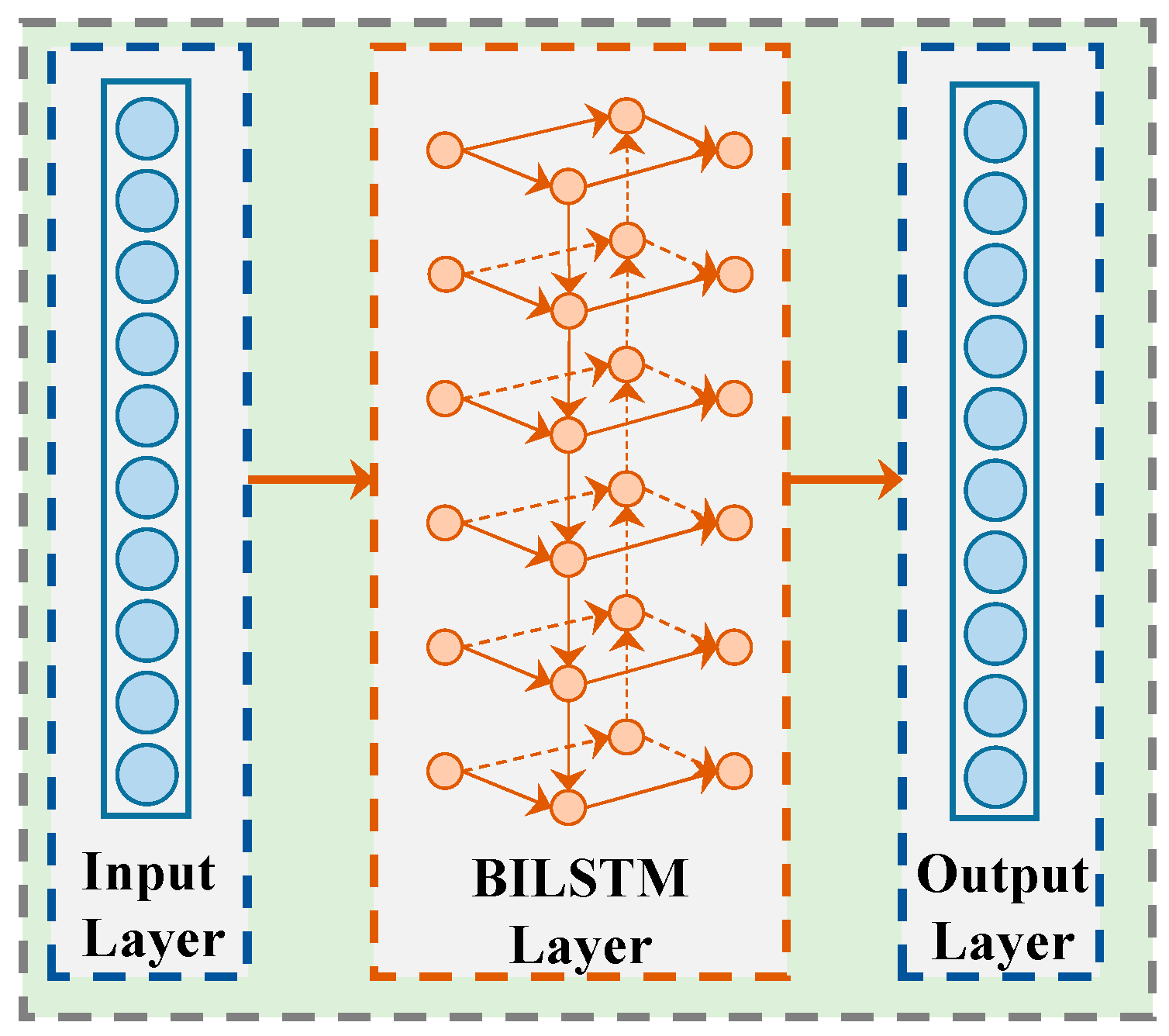
Since accommodation soft sensors utilize data directly sourced from the historical data of the faulty sensor, which exhibits a more direct and tighter correlation with the sensor values to be predicted, this allows for the attainment of more accurate prediction results. The structure of the BILSTM accommodation soft sensor is shown in Figure 5, consisting of the input layer, BILSTM layer, and output layer. The input variable is one-dimensional sensor data, as shown in Equation (9). The BILSTM layer and output layer are the same as in the diagnosis soft sensor and is not further elaborated.

$$x=\left[\begin{array}{c}{x}_1^1\\ x_1^2\\ ⋮\\ x_1^5\end{array}\right]$$

(9)

3. Experiment

In order to verify the feasibility of the proposed method, an HVAC sensor system data collection experiment was designed. Seven types of sensors were installed on the experimental platform. By diagnosing their bias faults and reconstructing faulty data, the proposed soft-sensor-based HVAC SFDIA scheme was validated. All experiments were conducted under refrigeration conditions in a standard enthalpy-difference laboratory.

3.1. Experimental Design

3.1.1. Experimental System

The HVAC system experimental platform consisted of a compressor, condenser, evaporator, bidirectional flow expansion valve, evaporator fan, condenser fan, control cabinet, and supervisory computer, as shown in Figure 6. Seven types of sensors were installed for the experiments, and their detailed descriptions are provided in

Table 1. Description of experimental sensors.

No.	Measure Location	Symbol	Unit
1	Outdoor inlet dry bulb temperature	T1	°C
2	Indoor outlet dry bulb temperature	T2	°C
3	Expansion valve inlet temperature	T3	°C
4	Expansion valve outlet temperature	T4	°C
5	Evaporator outlet temperature	T5	°C
6	Compressor discharge temperature	T6	°C
7	Condenser inlet temperature	T7	°C

. During the experiment, the system was turned on to ensure its normal operation. By adjusting the indoor and outdoor dry bulb temperatures, typical summer operating conditions were simulated. The indoor temperature was controlled within the range of 20 °C to 28 °C, while the outdoor temperature was adjusted between 28 °C and 38 °C.

3.1.2. Experiment Data Acquisition

The experimental data were collected at a frequency of 5 s. After removing outliers, a total of 5982 datasets were obtained, with 4982 sets used for the training dataset, 600 for the testing dataset, and 400 for the validation dataset. The sensor measurements consist of three components, as shown in Equation (10). In this equation, f_t represents the system error mainly caused by sensor faults. The focus of this study is primarily on bias faults in sensors, where a constant difference exists between the measured values from physical sensors and the true values. The mathematical model is given by Equations (11) and (12). Considering the sensor’s measurement precision, permissible error range, and the residual between the soft sensor and the physical sensor, the magnitude of bias faults is comprehensively taken into account. The testing dataset introduces faults into the diagnosed sensor from the 200th dataset, while the validation dataset introduces faults starting from the 100th dataset. The simulated scenarios of bias faults are presented in

Table 2. Simulated scenarios of sensor bias faults.

Faulty Sensors	Fault Level 1		Fault Level 2
	Positive Bias Fault	Negative Bias Fault	Positive Bias Fault	Negative Bias Fault
T1	0.6	−1	0.5	−0.9
T2	0.6	−0.3	0.5	−0.2
T3	1.8	−1.3	1.7	−1.2
T4	0.5	−0.6	0.4	−0.5
T5	0.7	−0.7	0.6	−0.6
T6	0.5	−0.5	0.4	−0.4
T7	0.6	−0.6	0.5	−0.5

. Given the low probability of multiple sensors failing simultaneously, this paper addresses the situation of single-sensor faults.

$$x_t=x_t^{*}+f_t+v_x$$

(10)

where x_t represents the measured value at time t, $x_t^{*}$ represents the true value at that moment, f_t stands for the system error, and v_x denotes the random error.

$$f_t=c$$

(11)

$$x_t=x_t^{*}+c+v_x$$

(12)

where c represents a constant.

3.2. Experiment Evaluation Metrics

The root-mean-square error (RMSE) and mean absolute error (MAE) are chosen as performance evaluation metrics to quantify the predictive performance of the proposed method against other models, as shown in Equations (13) and (14). The RMSE indicates the dispersion of samples. The MAE measures the absolute error between predicted values and observed values.

$$MAE=\frac{1}{m}\sum _{i=1}^m\left|\left(f_i-y_i\right)\right|$$

(13)

$$RMSE=\sqrt{\frac{1}{m}\sum _{i=1}^m{(f_i-y_i)}^2}$$

(14)

where f_i represents the predicted value, y_i represents the true value, and m is the sample count.

To quantitatively assess the diagnostic performance of sensor faults, the false alarm rate (FAR) is introduced to evaluate cases where normal sensor samples are incorrectly diagnosed as faulty samples, and the fault detection rate (FDR) is used to evaluate the detection of faulty sensor samples. The formulas are provided by Equations (15) and (16), respectively.

$$FAR=\frac{\mathrm{N}\mathrm{u}\mathrm{m}\mathrm{b}\mathrm{e}\mathrm{r} \mathrm{o}\mathrm{f} \mathrm{n}\mathrm{o}\mathrm{r}\mathrm{m}\mathrm{a}\mathrm{l} \mathrm{s}\mathrm{a}\mathrm{m}\mathrm{p}\mathrm{l}\mathrm{e}\mathrm{s} \mathrm{r}\mathrm{e}\mathrm{p}\mathrm{o}\mathrm{r}\mathrm{t}\mathrm{e}\mathrm{d} \mathrm{a}\mathrm{s} \mathrm{f}\mathrm{a}\mathrm{u}\mathrm{l}\mathrm{t}\mathrm{s}}{\mathrm{T}\mathrm{o}\mathrm{t}\mathrm{a}\mathrm{l} \mathrm{n}\mathrm{u}\mathrm{m}\mathrm{b}\mathrm{e}\mathrm{r} \mathrm{o}\mathrm{f} \mathrm{n}\mathrm{o}\mathrm{r}\mathrm{m}\mathrm{a}\mathrm{l} \mathrm{s}\mathrm{a}\mathrm{m}\mathrm{p}\mathrm{l}\mathrm{e}\mathrm{s}}=\frac{FP}{FP+TN}$$

(15)

$$FDR=\frac{\mathrm{N}\mathrm{u}\mathrm{m}\mathrm{b}\mathrm{e}\mathrm{r} \mathrm{o}\mathrm{f} \mathrm{f}\mathrm{a}\mathrm{u}\mathrm{l}\mathrm{t} \mathrm{s}\mathrm{a}\mathrm{m}\mathrm{p}\mathrm{l}\mathrm{e}\mathrm{s} \mathrm{r}\mathrm{e}\mathrm{p}\mathrm{o}\mathrm{r}\mathrm{t}\mathrm{e}\mathrm{d} \mathrm{a}\mathrm{s} \mathrm{n}\mathrm{o}\mathrm{r}\mathrm{m}\mathrm{a}\mathrm{l}}{\mathrm{T}\mathrm{o}\mathrm{t}\mathrm{a}\mathrm{l} \mathrm{n}\mathrm{u}\mathrm{m}\mathrm{b}\mathrm{e}\mathrm{r} \mathrm{o}\mathrm{f} \mathrm{f}\mathrm{a}\mathrm{u}\mathrm{l}\mathrm{t} \mathrm{s}\mathrm{a}\mathrm{m}\mathrm{p}\mathrm{l}\mathrm{e}\mathrm{s}}=\frac{TP}{TP+FN}$$

(16)

where TP represents True Positive samples; FP represents False Positive samples; FN represents False Negatives; and TN represents True Negatives.

The fault diagnosis results are directly linked to the fault threshold. In order to achieve better fault diagnosis performance, characterized by higher fault detection rates and lower false alarm rates, the difference between the fault detection rate and the false alarm rate is defined as the fault threshold performance evaluation metric, as presented in Equation (17). The range of the score is [−1, 1]. When the score is close to 1, it indicates that the method has a higher fault detection rate and lower false alarm rate.

$$score=FDR-FAR$$

(17)

The data recovery performance is evaluated using the RMSE and the coefficient of determination (R²), as shown in Equations (14) and (18), respectively. The RMSE is used to measure the distance between reconstructed data and true value. R² is used to measure the similarity between two signals, where R² closer to 1 indicates a higher similarity between the two signals, implying that the reconstructed sensor data effectively represent the true value.

$$R^2=1-\frac{\sum _{t=1}^n{\left(y_t-\overline{y_t}\right)}^2}{\sum _{t=1}^n{\left(y_t-\dot{y}\right)}^2}$$

(18)

4. Results Analysis

4.1. Analysis of Fault Diagnosis Results Based on Soft Sensor

A CNN-BILSTM-ATTENTION-based soft sensor is constructed using the training dataset of six sensors, excluding the diagnosed sensor. Different models’ predictive performances are compared on the test set to identify the model with the best predictive results. The optimal fault threshold is determined using the testing set. Finally, the feasibility of the approach is validated by conducting fault diagnosis on the validation set.

4.1.1. Analysis of Prediction Results

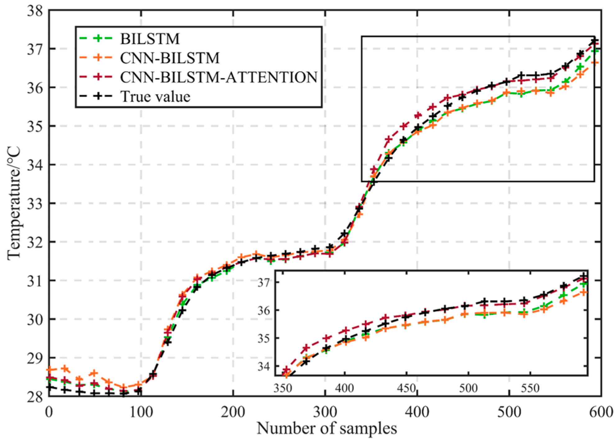
On the testing dataset, diagnosis soft sensors are employed to predict the values of seven sensors. The comparison chart of predicted results for the T₁ sensor is presented in Figure 7. The soft sensor built with CNN-BILSTM-ATTENTION exhibits a better representation of the changing trends of the true values.

Table 3. Predictive evaluation metric results for different models.

Sensor	Results of Predictive Evaluation Metrics for Different Models
	BILSTM		CNN-BILSTM		CNN-BILSTM-ATTENTION
	MAE	RMSE	MAE	RMSE	MAE	RMSE
T1	0.1772	0.2167	0.2397	0.2896	0.1446	0.1872
T2	0.1647	0.1822	0.1687	0.1845	0.1223	0.1370
T3	0.6136	0.7541	0.6530	0.7587	0.3306	0.4398
T4	0.2054	0.2546	0.1264	0.1473	0.0985	0.1305
T5	0.2095	0.2447	0.2169	0.2504	0.1830	0.2361
T6	0.2194	0.2564	0.1309	0.1608	0.1040	0.1381
T7	0.0962	0.1268	0.1556	0.1847	0.0904	0.1093
Average value	0.2409	0.2908	0.2416	0.2823	0.1533	0.1969

presents a comparative analysis of prediction evaluation metrics for soft sensors built using different models. The CNN-BILSTM-ATTENTION model consistently achieves the best results across all metrics, with average MAE and RMSE reductions of 30.51% and 25.03%, respectively, compared to other optimal results. As a result, CNN-BILSTM-ATTENTION stands as the optimal diagnosis soft sensor prediction model.

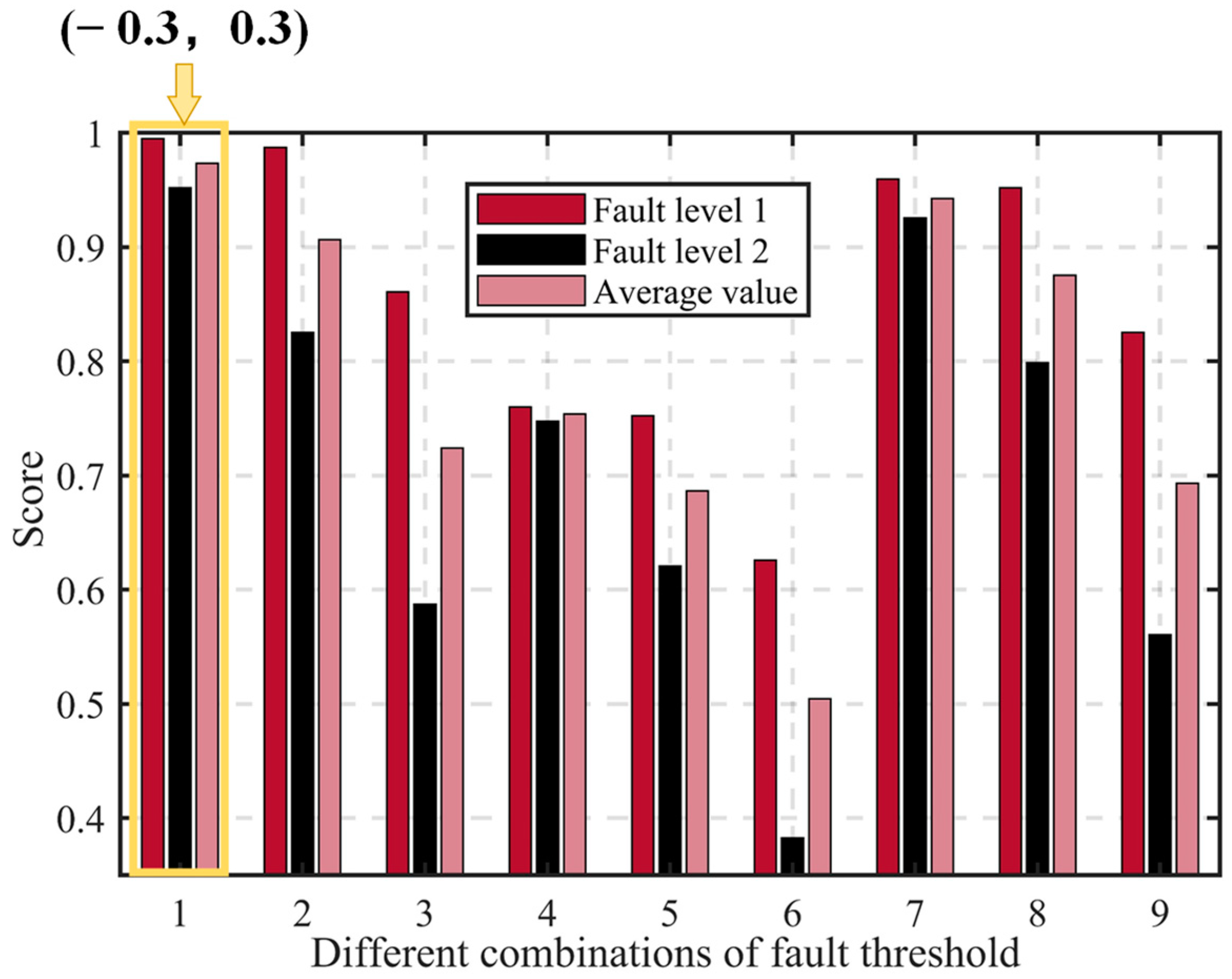
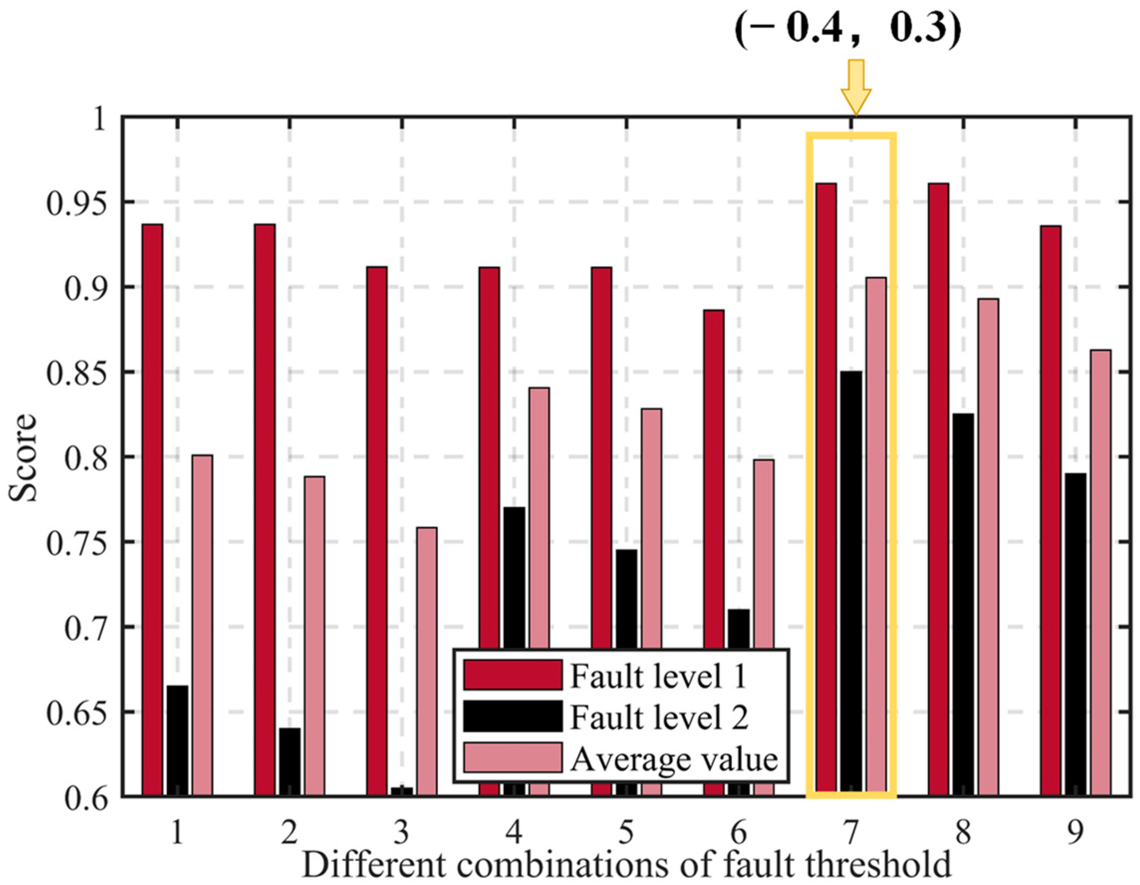
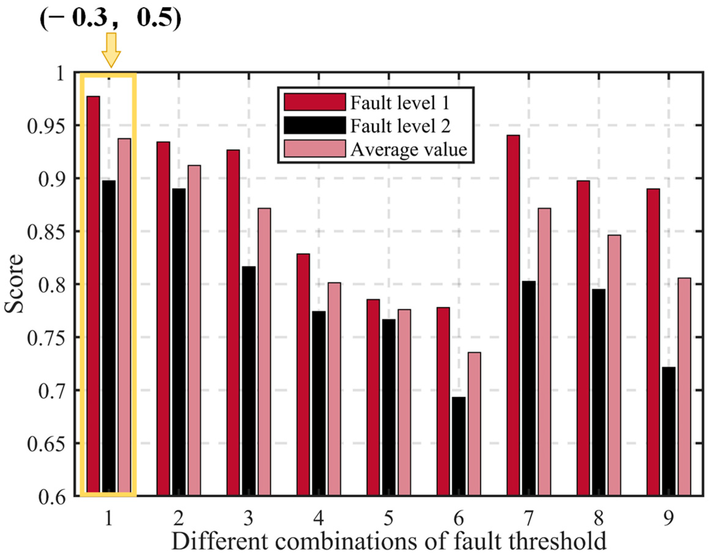
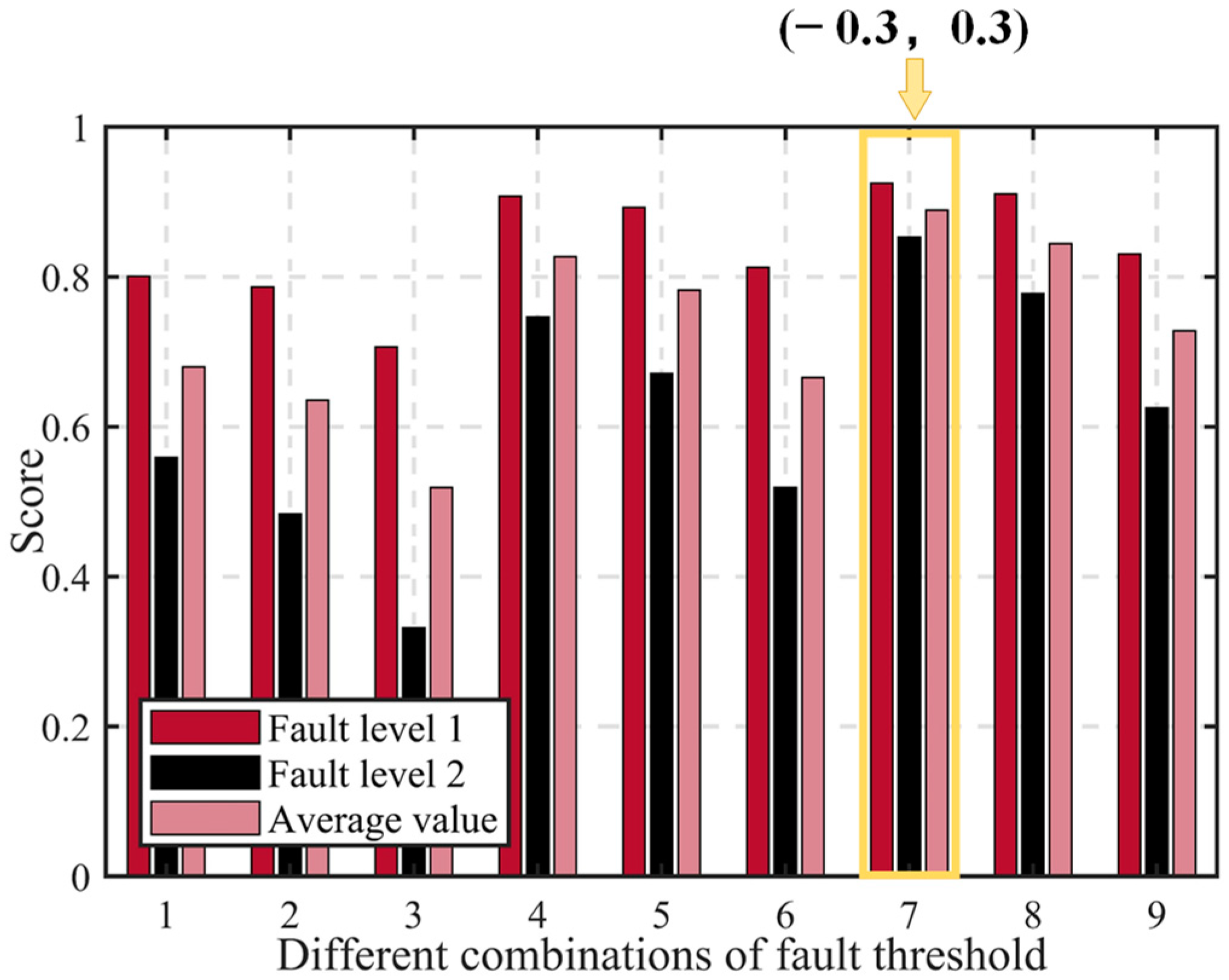
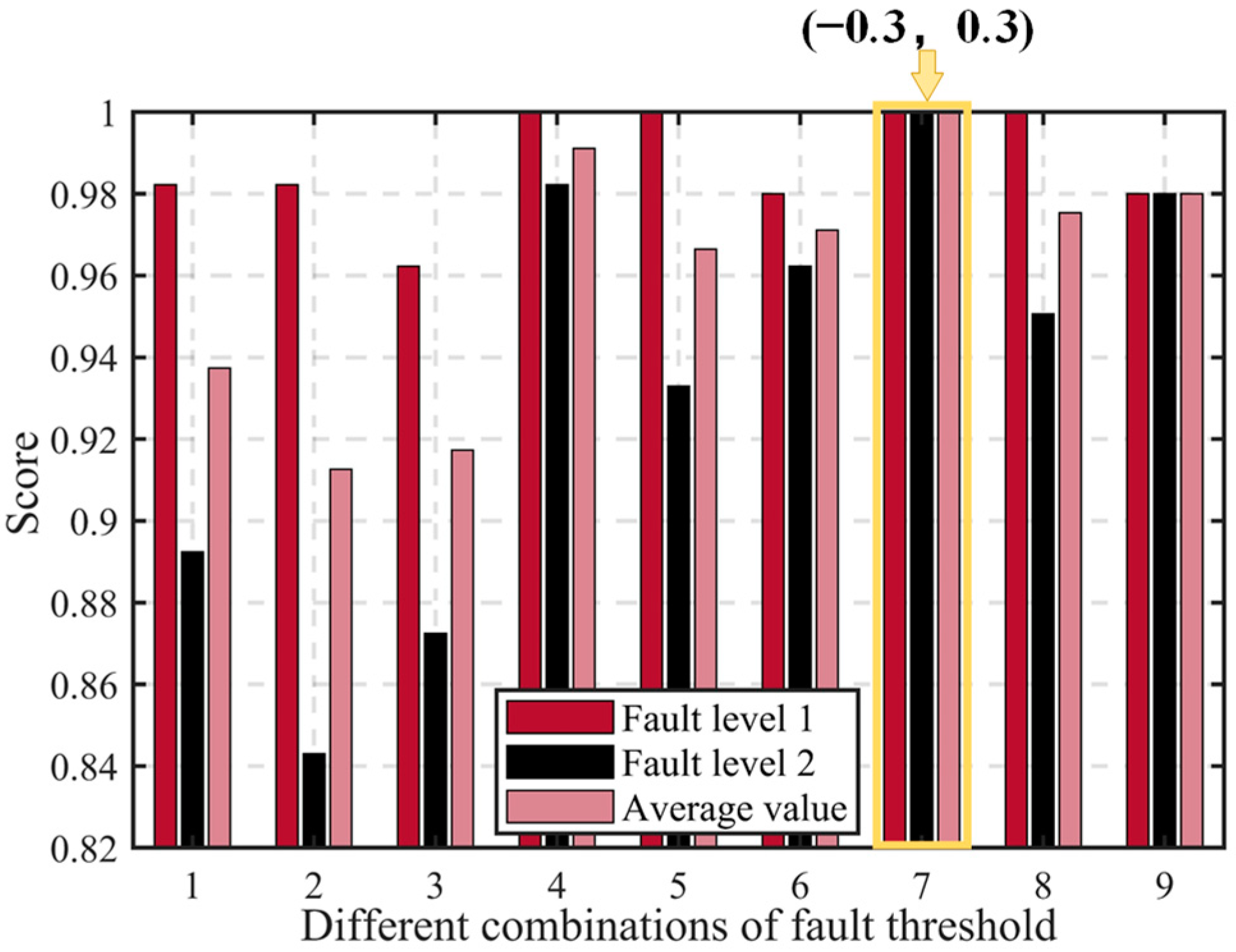
4.1.2. Analysis of Fault Threshold and Diagnosis Results

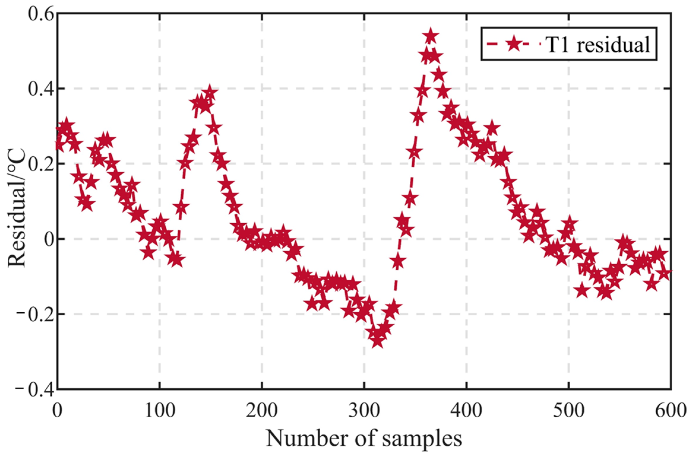
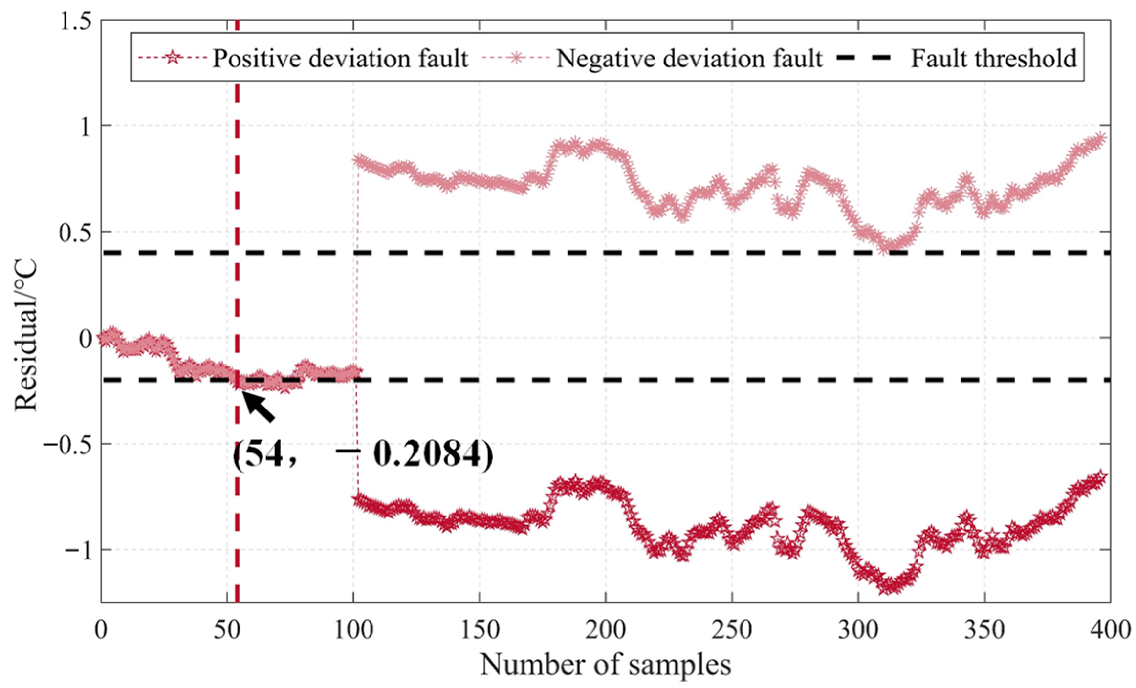
To maximize the fault diagnosis performance, the score is used to determine the optimal fault threshold. Firstly, the residual between the output of the soft sensor and the measurement of the physical sensor is calculated, as in Equation (19), to determine the difference caused by the predictive model. Figure 8 illustrates the residuals of the T₁ sensor. Currently, many diagnostic methods use the maximum residual value as the fault threshold. Although using the maximum value as the fault threshold can achieve a lower false alarm rate, it also decreases the fault detection rate, thus failing to achieve the best diagnostic outcome. Therefore, to select a more suitable fault threshold, the range of the fault threshold can be preliminarily determined based on the distribution of residuals. For instance, the positive threshold range for the T₁ sensor is [0.4~0.6], and the negative threshold range is [−0.2~−0.4]. Introducing faults into the test set, a test is conducted to determine the optimal fault threshold. By adjusting the thresholds within the defined positive and negative threshold ranges, false alarm rates and fault detection rates are computed for different threshold combinations. The fault threshold yielding the best score is chosen. 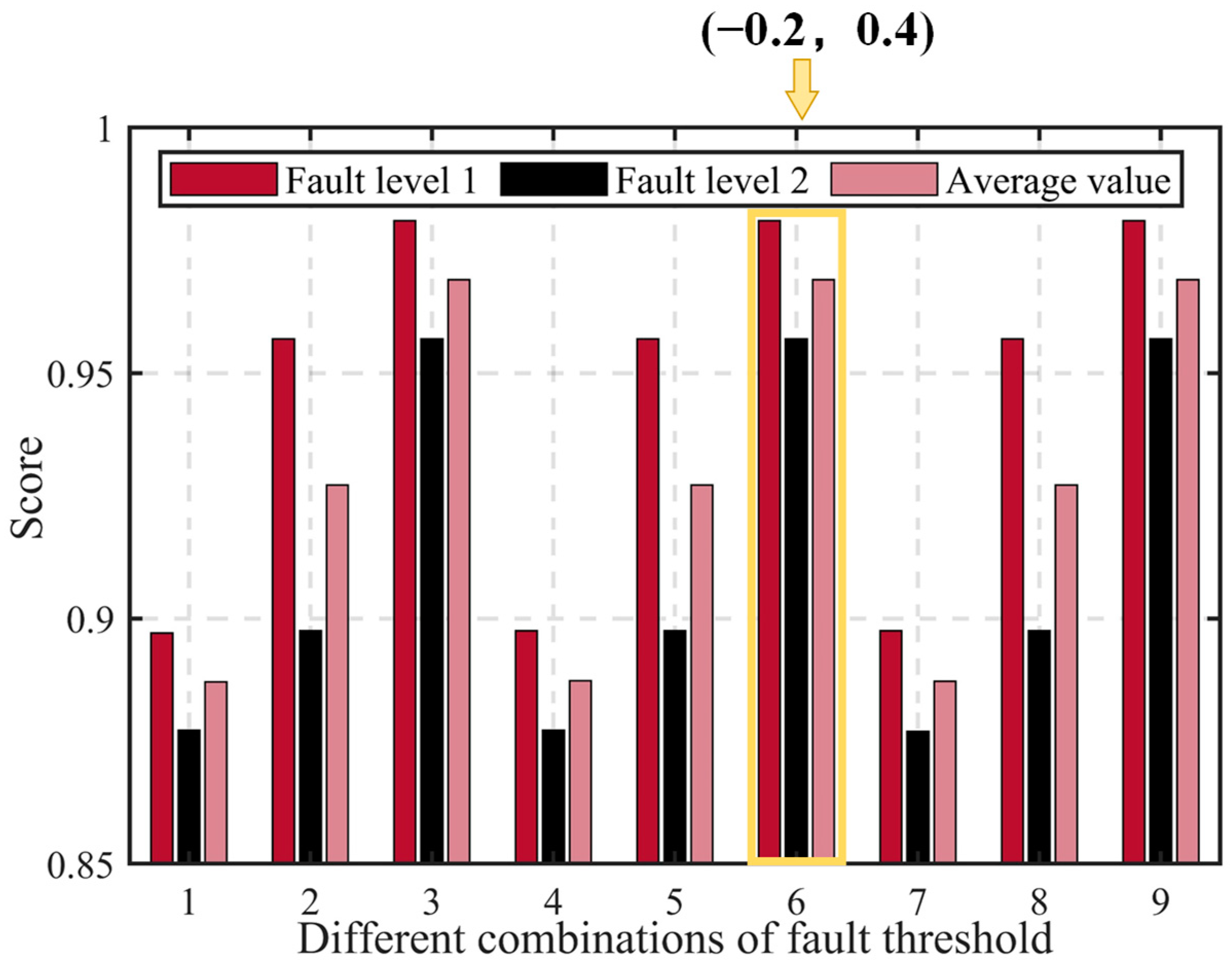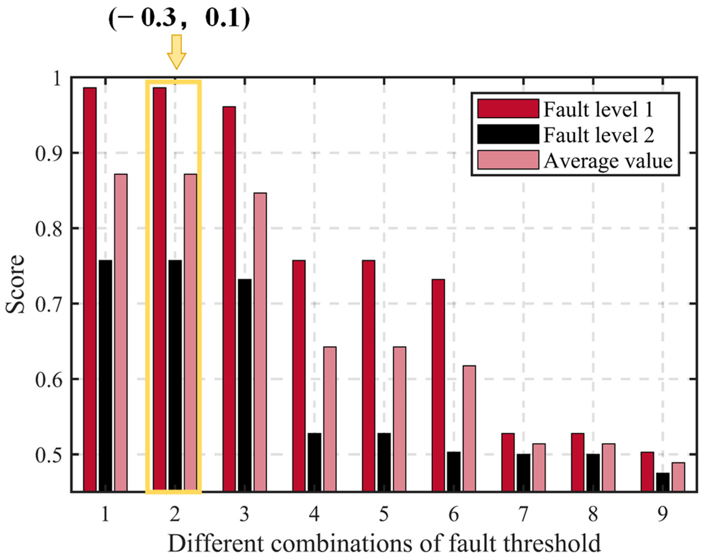Figure 9, Figure 10, Figure 11, Figure 12, Figure 13, Figure 14 and Figure 15 present a comparison of the score results for different threshold combinations. When the score metric is equal, the threshold combination with the narrower range is selected to achieve more precise fault diagnosis. Using the optimal threshold, fault diagnosis is performed on the validation set to validate the performance of the best threshold combination and the effectiveness of the fault diagnosis method proposed. The validation set’s fault diagnosis results are depicted in Figure 16, Figure 17 and Figure 18.

$$\epsilon =y_{prediction}-y_{physics}$$

(19)

where y_prediction represents the output of the soft sensor and y_physics represents the measurement of the physical sensor.

Therefore, soft sensors can effectively predict sensor data, which enable the implementation of fault diagnosis and realize good performance.

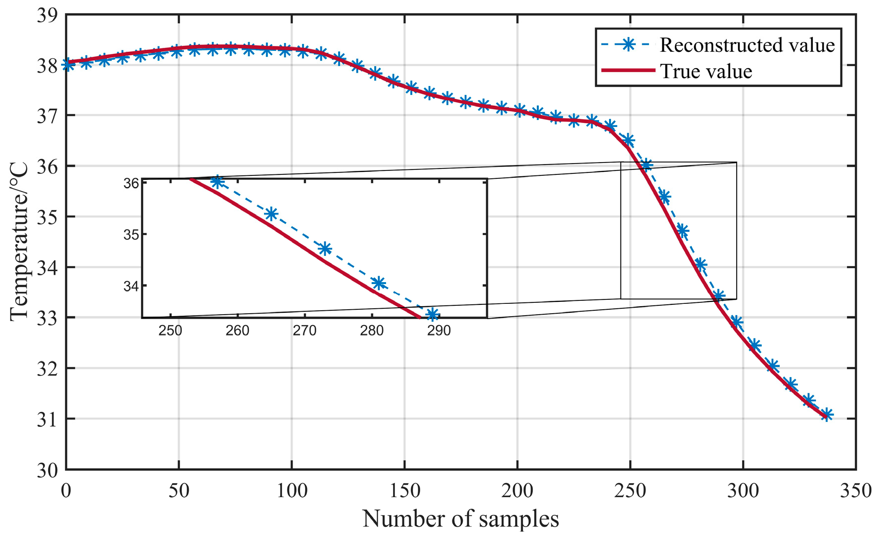
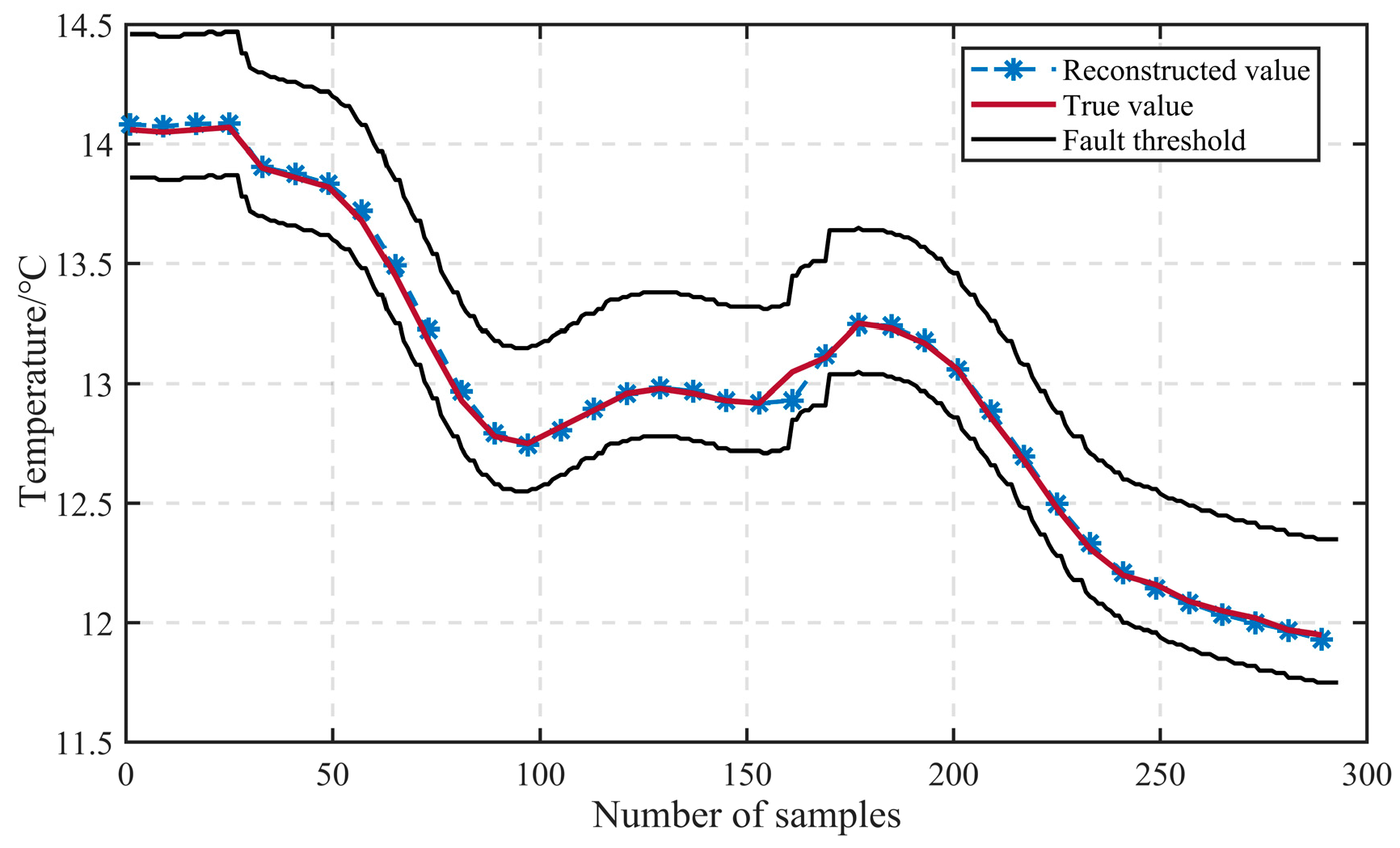
4.2. Analysis of Fault Accommodation Results Based on Soft Sensor

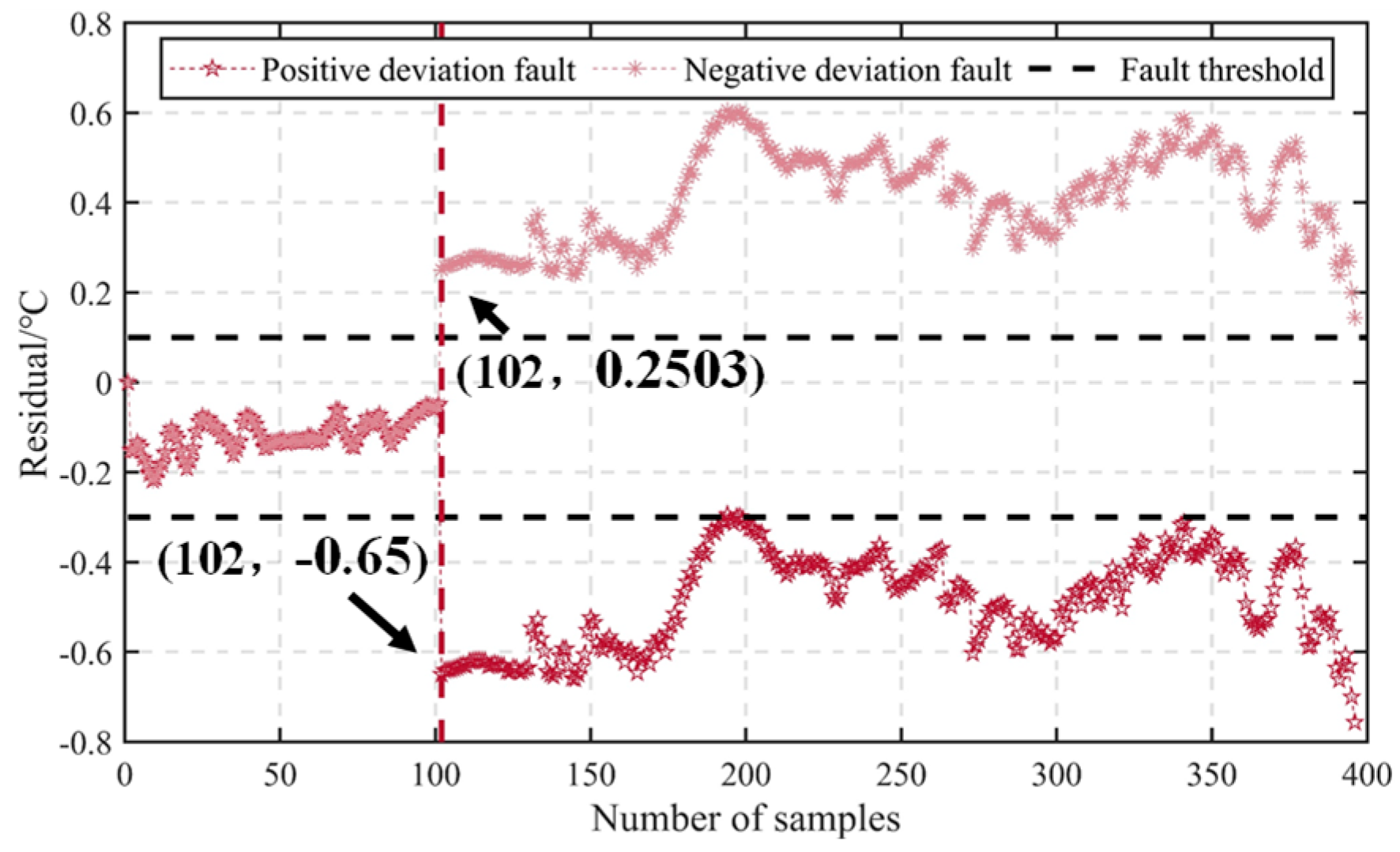
Faulty sensor data can impact the operational performance of the HVAC system. Thus, accurate identification of sensor fault points is essential. Data recovery is initiated from this point. Figure 19 and Figure 20 illustrate the results of identifying fault locations for the T₁ and T₂ sensors. In the validation dataset, faults are introduced from the 100th data point, and the first five continuous data points exceeding the fault threshold should correspond to the 102nd data point, as shown in the T₂ sensor identification result. Taking the T₁ sensor as an example, some sensors identify normal states as faults. In such cases, recovery is performed on normal data (normal data are falsely identified as faulty data). However, this case occurs rarely, and the recovered data remain within the fault threshold, making it viable to treat as normal data. The recovered data from each sensor fall within the fault threshold range. The data recovery results for the T₁ and T₂ sensors are shown in Figure 21 and Figure 22. The reconstructed data represent the output of the soft sensor and closely resemble the true data. Figure 22 indicates that the reconstructed data fall within the fault threshold range and are considered normal data. This implies that the reconstructed data can effectively recover faulty data.

Table 4. Evaluation results of fault sensor accommodation.

Sensor	T1	T2	T3	T4	T5	T6	T7
MAE	0.0685	0.0181	0.0746	0.0278	0.0336	0.0806	0.0641
RMSE	0.0968	0.0247	0.1026	0.0433	0.0472	0.1135	0.0886

provides the evaluation results of using the soft sensor for data recovery.

The results indicate that when sensors experience faults, compared with diagnosis soft sensors, accommodation soft sensors exhibit smaller predictive evaluation metrics. In other words, its predictive performance is better, and its predictions are closer to true data. It can effectively substitute true data, thereby achieving the reconstruction and recovery of faulty data.

4.3. Discussion

Based on the experimental results of the aforementioned fault diagnosis and accommodation, the following conclusions can be drawn:

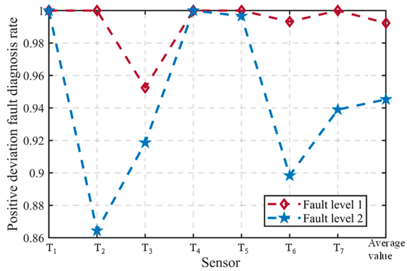
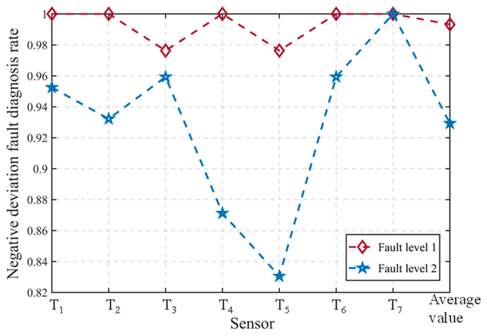
(1) The fault diagnosis method can achieve good diagnostic results for faults of different levels. The larger the fault level, the more pronounced the fault manifestation, resulting in better diagnostic outcomes. The diagnostic performance for fault level 1 is noticeably superior to that of fault level 2.

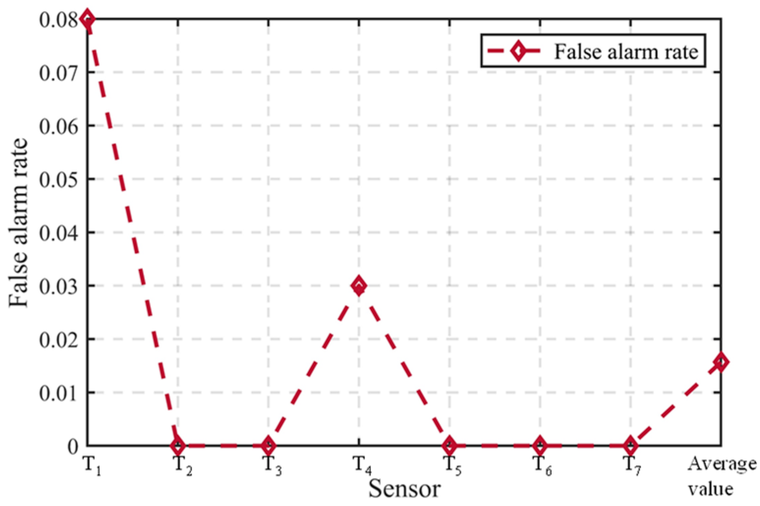
(2) The utilization of the best fault thresholds selected using the score obtains better fault diagnosis outcomes, with an average false alarm rate of 1.57%, an average positive deviation fault detection rate of 96.88%, and an average negative deviation fault detection rate of 96.13%.

(3) For faulty sensors, the method is capable of effectively identifying the fault location. Utilizing single-variable input soft sensors, the faulty data can be successfully recovered. The reconstructed data fall within the fault threshold range, enabling short-term data recovery and maintaining the proper functioning of the HVAC systems.

5. Conclusions

In this article, a scheme for sensor diagnosis, isolation, and accommodation in HVAC systems using soft sensors is used to provide an accurate evaluated value of a physical sensor based on available physical sensors. The scheme only requires fault-free training data during normal operation, without needing a detailed understanding of the characteristics of sensor fault signals. Additionally, by utilizing a defined score metric to quantitatively select the most appropriate threshold, higher fault detection rates and lower false alarm rates are achieved. Soft sensors provide a very effective and promising method for HVAC SFDIA.

Apart from sensor faults, actuator faults, control software programming faults, and stationary part faults are also common occurrences in HVAC systems [28]. Future work could further investigate how to decouple composite faults in soft sensor design. In addition, using multi-source sensor data fusion and information mutual verification and complementary technology to realize sensor fault diagnosis, it may be more advantageous in complex systems requiring high reliability and comprehensiveness.