Variational Reduced-Order Modeling of Thermomechanical Shape Memory Alloy Based Cooperative Bistable Microactuators

Abstract

This article presents the formulation and application of a reduced-order thermomechanical finite strain shape memory alloy (SMA)-based microactuator model for switching devices under thermal loading by Joule heating. The formulation is cast in the generalized standard material framework with an extension for thermomechanics. The proper orthogonal decomposition (POD) is utilized for capturing a reduced basis from a precomputed finite element method (FEM) full-scale model. The modal coefficients are computed by optimization of the underlying incremental thermomechanical potential, and the weak form for the mechanical and thermal problem is formulated in reduced-order format. The reduced-order model (ROM) is compared with the FEM model, and the exemplary mean absolute percentage errors for the displacement and temperature are $0.973\%$ and $0.089\%$, respectively, with a speedup factor of $9.56$ for a single SMA-based actuator. The ROM presented is tested for single and cooperative beam-like actuators. Furthermore, cross-coupling effects and the bistability phenomenon of the microactuators are investigated.

1. Introduction

Since the discovery of shape memory alloys (SMAs), they have been used in various applications. For example, as orthodontic appliances, in mobile phones, valves, space robotics and microactuators [1,2]. Their frequent use in these applications stems from their unique properties, namely the super-elasticity and the shape memory effect [3,4,5,6]. SMA-based microactuators are in increased demand [7,8] because they have a high mechanical strength and work density, which results in lightweight structures that can repeatedly generate large forces with small device sizes [9,10]. SMA-based actuators have the disadvantage of low actuation speed caused by the latency of thermal cooling, which is strongly size-dependent. Song et al. [11] proposed a smart soft composite actuator that is capable of large deformations with fast bending actuation. Stachiv et al. [12] proposed an approach to use SMA in combination with an elastic substrate as tunable active layer. Samal et al. [13] investigated the bending stiffness and radius of curvature of polymethyl methacrylate (PMMA) and NiTi SMA composites upon application of an external thermal load. The discussed actuator in this paper is based on a concept explored by Winzek et al. [14]. They investigated a combination of SMA and polymer that leads to the actuator behaving in a bistable manner.

These SMA-based actuators usually undergo transformation due to a thermal loading during their operation. Therefore, it is necessary to understand the complex, nonlinear thermomechanical behavior of the SMA-based actuator, which makes the numerical implementation challenging [15].

The shape memory and super-elastic effect occur in SMAs due to a phase transformation between austenite and martensite, which is induced by thermomechanical loadings [9,16,17,18]. SMA models can be developed based on a continuum thermodynamics framework. In this work, we take into account the thermomechanical potential developed by Yang et al. [19] and assume a potential including internal variables [5,17,20]. Sielenkämper et al. [21] extended the SMA potential formulation from Sedlak et al. [22] to the finite strain case, which was developed for small-strain SMA modeling. It captures the super-elasticity and shape memory effect, as well as the volume change due to phase transformation, which is found in some SMAs [23]. Frost et al. [24] also developed a thermomechanical model for SMAs within the framework of generalized standard materials that could predict the martensite transformation and its localization. Solomou et al. [25] proposed a coupled thermomechanical SMA-based actuator model that is capable of simulating heat transfer and convection effects in the actuator. There, the constitutive equations for SMAs from Lagoudas’ model [10] are used to predict the coupled thermomechanical response of an SMA beam.

It is often time-consuming to perform an experimental investigation for the design optimization of new components [26]. For nonlinear multiphysics problems, such optimizations are usually perceived by numerical simulations [27,28], which might have millions of degrees of freedom (DOF), and can thus be computationally expensive [29] and also require a continuously evolving discretized model for nonlinear problems [30,31,32]. Performing simulations using an FEM model sometimes becomes unfeasible when performing hundreds of simulations for different, varying parameters such as different loading conditions, different values of Young’s modulus and Poisson’s ratio to design a new structure [26,33]. Therefore, we need a reduced-order model to reduce the computational cost with respect to solving parametrized nonlinear partial differential equations (PDEs) [32]. Different model order reduction techniques that perform well in reducing the computational time while preserving model accuracy have been utilized. Model order reduction (MOR) is a class of techniques to approximate a higher dimensional system by a low-dimensional model [26]. POD has been utilized by many researchers as a basis for MOR techniques [34,35,36].

Reduced-order modeling for a compact FEM model could speed up the investigation process significantly while keeping a certain level of model accuracy. Vettermann et al. [37] developed a strategy for coupled thermomechanical problems with nonlinear boundary conditions for faster simulations of machine tools. Ummunakwe et al. [38] developed a reduced-order thermomechanical model for packaged chips using Krylov subspace methods with excellent model accuracy.

JinXiu et al. [39] used POD to analyze transient heat conduction problems and proposed a fast reduced-order model that could interpolate and extrapolate the field variable at an unknown time. Jia et al. [40] proposed a reduced-order thermal model for a multifin field effect transistor, which provides accurate solutions. Bikora et al. [41] developed a low-order model to predict the thermal deformation in reticles for extreme ultraviolet lithography, which is based on a large-scale thermomechanical FEM model. Hernandez et al. [42] worked on a thermomechanical reduced-order model for machine tools that predicts the thermal response in a frequency range and also predicts the coupling between the mechanical and thermal responses. Das et al. [43] proposed a thermomechanical reduced-order model using POD to simulate the thermomechanical processes that occur during the fabrication of photovoltaic cells.

The objective of this paper is to develop a fast and reliable reduced-order model for the FEM model developed by Sielenkämper et al. [21]. The novelty of this ROM is the application to the coupled thermomechanical potential, which was first considered by Yang et al. [19]. First, samples of snapshots are generated from high-fidelity FEM solutions for different parameter sets. This so-called offline computation is computationally expensive. Subsequently, a reduced basis that could best represent the full snapshot matrix is obtained from the snapshots through statistical tools. Then, the most significant modes contained in the reduced basis are used to predict the overall behavior of the nonlinear SMA actuator model.

The article is organized as follows: The second section provides, in compact form, all necessary equations for the thermomechanical SMA-based model. Then, a reduced-order model is presented. Section 3 presents the application of the ROM to different examples. Finally, Section 4 concludes the paper, along with suggestions for future work.

We used bold letters for first- and second-order tensors, as well as tensor-valued functions such as $\mathit{P}$, and light face letters for scalars and scalar valued functions such as T.

2. Modeling of the Thermomechanical SMA-Based Actuator

This section briefly presents the mathematical formulation for the SMA-based actuator model.

2.1. Continuum Model

Within a continuum body with reference configuration ${\mathcal{B}}_0$, the displacement vector $\mathit{u}$ of a material point with reference position vector $\mathit{X}$ at time t is defined as the difference between the current and reference position vectors $\mathit{x}$ and $\mathit{X}$, respectively ($\mathit{u}(\mathit{X},t)=\mathit{x}(\mathit{X},t)-\mathit{X}$). The deformation gradient $\mathit{F}$ describes the mapping of infinitesimal line elements from the reference to the current configuration and can be expressed as

$$\mathit{F}=\mathrm{Grad}(\mathit{x}(\mathit{X},t))$$

(1)

In the reference configuration, the linear momentum balance for a body ${\mathcal{B}}_0$ can be written as

$$\mathrm{Div}\mathit{P}+{\rho }_0\mathit{b}=\mathbf{0},$$

(2)

where $\mathit{b}$ is the body force, ${\rho }_0$ is the reference mass density and $\mathit{P}$ is the first Piola–Kirchoff stress tensor. The boundary conditions are $\mathit{u}=\overline{\mathit{u}}$ on $\partial {\mathcal{B}}_{0u}$ and $\widehat{\mathit{t}}=\mathit{PN}$ on $\partial {\mathcal{B}}_{0t}$, with the given traction vector $\widehat{\mathit{t}}$ and the external normal $\mathit{N}$ in the reference configuration.

We consider the free energy density (with respect to the reference configuration) $\psi =\psi (\mathbf{C},T,\mathbf{Z})$, which depends on the right Cauchy–Green tensor $\mathit{C}={\mathit{F}}^T\mathit{F}$, the absolute temperature T and an array of internal variables $\mathbf{Z}$. Inserting this function into the Clausius–Planck inequality and using Coleman and Noll’s reasoning, we can write

$$\mathit{P}=\frac{\partial \psi }{\partial \mathit{F}};s=-\frac{\partial \psi }{\partial T},$$

(3)

where s denotes the entropy density per unit reference volume.

We assume a scalar dissipation potential for the isothermal case (the nonisothermal case is discussed below, see Equation (7)) $\varphi (\dot{\mathbf{Z}},\mathbf{Z})$ to depend on internal variables $\mathbf{Z}$ and the rate of the internal variables $\dot{\mathbf{Z}}$. For general standard dissipative solids, the rates of the internal variables are identified by solving Biot’s equation

$$\frac{\partial \psi }{\partial \mathbf{Z}}+\frac{\partial \varphi }{\partial \dot{\mathbf{Z}}}\ni \mathbf{0},$$

(4)

where $\partial \varphi /\partial \dot{\mathbf{Z}}$ in general denotes a subdifferential. We obtain the dissipation density as

$$\mathcal{D}=\frac{\partial \varphi (\dot{\mathbf{Z}},\mathbf{Z})}{\partial \dot{\mathbf{Z}}}·\dot{\mathbf{Z}}.$$

(5)

Then, the balance of energy with Fourier’s law, for simplicity taken as $\mathit{Q}=-\kappa \mathrm{Grad}T$, where $\kappa$ is the heat conductivity and $\mathit{Q}$ is the heat flux vector in the reference configuration, can be represented as

$$T\dot{s}=-\mathrm{Div}(\kappa \mathit{Q})+w+\mathcal{D},$$

(6)

where w represents the heat source density. The Dirichlet boundary condition for the thermal part is $T=\overline{T}$ on $\partial {\mathcal{B}}_{0T}$. The Robin-type boundary condition is given as $\mathit{Q}·\mathit{N}=\alpha (T-T_a)$ on $\partial {\mathcal{B}}_{0Q}$. Here, $\alpha$ is the heat transfer coefficient and $T_a$ is the ambient temperature. Neumann-type boundary conditions are not considered.

Consider the following rate potential for the nonisothermal case in its time-discrete format for the material modeling of the SMA (compare Yang et al. [19]).

$$\psi (\mathbf{C},T,\mathbf{Z})-(e_n-T{s}_n)+\Delta t\varphi \left(\frac{T}{T_n}\mathring{\mathbf{Z}},\mathbf{Z}\right),$$

(7)

where $e_n$ and $s_n$ are the internal energy density and entropy density at time $t_n$, respectively. $\mathring{\mathbf{Z}}$ is a numerical approximation of the time derivative of $\mathbf{Z}$. This means that any $\mathring{\mathbf{Z}}$ satisfying ${lim}_{\Delta t\to 0}\mathring{\mathbf{Z}}=\dot{\mathbf{Z}}$ is admissible. A typical example is $\mathring{\mathbf{Z}}=\Delta \mathbf{Z}/\Delta t$. Additionally, $\Delta t\varphi$ is denoted as ${\varphi }_{\Delta }$ and is assumed homogeneous of degree one in its first variable in the following. Note that the major difference of the dissipation potential in the nonisothermal case compared with the isothermal case is the factor $T/T_n$ in the first argument.

The temperature and the displacement vector are the unknown state variables. Fourier’s heat conduction law is assumed along with dissipative terms. Both state variables are coupled through the following time-discrete potential

$${\pi }_{\Delta }=\psi -(e_n-T{s}_n)+{\varphi }_{\Delta }-\kappa \frac{\Delta t}{2T_n}{\parallel \mathrm{Grad}T\parallel }^2+\kappa \frac{\Delta tT}{T_n^2}{\parallel \mathrm{Grad}{T}_n\parallel }^2,$$

(8)

where the last two terms in Equation (8) represent the heat conduction in the body. The integral form of the incremental potential is expressed as follows:

$${\Pi }_{\Delta }={\int }_{{\mathcal{B}}_0}{\pi }_{\Delta }\mathrm{d}V-{\int }_{\partial {\mathcal{B}}_{0t}}\widehat{\mathit{t}}·\mathit{u}\mathrm{d}S-{\int }_{{\mathcal{B}}_0}{\rho }_0\mathit{b}·\mathit{u}\mathrm{d}V-{\int }_{\partial {\mathcal{B}}_{0Q}}\frac{\alpha \Delta t}{2T_n}{(T-T_n)}^2\mathrm{d}S+{\int }_{{\mathcal{B}}_0}\Delta t\frac{T}{T_n}w\mathrm{d}V.$$

(9)

Now, the state variables and internal variables are obtained by solving the following saddle point problem

$$\underset{\mathit{u}\in {\kappa }_u}{inf}\underset{T\in {\kappa }_T}{sup}\underset{\mathbf{Z}}{inf}{\Pi }_{\Delta }.$$

(10)

Here, ${\kappa }_u=\{\mathit{u}:\mathit{u}=\overline{\mathit{u}}\mathrm{on}\partial {\mathcal{B}}_{0u}\}$ is the set of admissible displacement values fulfilling the Dirichlet boundary conditions on the boundary $\partial {\mathcal{B}}_{0u}$, and ${\kappa }_T=\{T:T=\overline{T}\mathrm{on}\partial {\mathcal{B}}_{0T}\}$ is the set of admissible temperatures that fulfill the Dirichlet boundary conditions on the boundary $\partial {\mathcal{B}}_{0T}$.

The weak form of the quasi-static linear momentum balance can be obtained by applying a variation of the potential with respect to the displacement:

$${\delta }_u{\Pi }_{\Delta }={\int }_{{\mathcal{B}}_0}\mathit{P}:\delta \mathit{F}\mathrm{d}V-{\int }_{\partial {\mathcal{B}}_{0t}}\widehat{\mathit{t}}·\delta \mathit{u}\mathrm{d}S-{\int }_{{\mathcal{B}}_0}{\rho }_0\mathit{b}·\delta \mathit{u}\mathrm{d}V,$$

(11)

where $\delta \mathit{F}$ and $\delta \mathit{u}$ are the variations of the deformation gradient and displacement vector, respectively. In the same way, the weak form of the energy balance can be obtained by the variation with the temperature T as follows:

$$\begin{array}{c}\hfill {\delta }_T{\Pi }_{\Delta }={\int }_{{\mathcal{B}}_0}(\left(\frac{\partial \psi }{\partial T}+s_n+\frac{1}{T_n}{\varphi }_{\Delta }(\mathring{\mathbf{Z}},\mathbf{Z})\right)\delta T-\frac{\kappa \Delta t}{T_n}\mathrm{Grad}(T)·\mathrm{Grad}(\delta T)\hfill \\ \hfill +\Delta t\frac{\delta T}{T_n^2}\kappa {\parallel \mathrm{Grad}(T_n)\parallel }^2+\frac{\Delta t}{T_n}w)\delta T\mathrm{d}V-{\int }_{{\mathcal{B}}_{0Q}}\alpha \frac{\Delta t}{T_n}(T-T_n)\delta T\mathrm{d}S=0.\end{array}$$

(12)

It can be easily verified that Equations (11) and (12) yield Equations (2) and (6), as well as the corresponding boundary conditions in the limit $\Delta t\to 0$, which proves the consistency of the time-discrete potential with the time-continuous theory.

Furthermore, the variation of the potential with respect to the internal variables yields the nonisothermal form of Biot’s equation, which represents the stationarity condition with respect to the internal variables:

$${\delta }_{\mathbf{Z}}{\Pi }_{\Delta }=\frac{\partial \psi }{\partial \mathbf{Z}}+\Delta t\frac{\partial \varphi }{\partial \mathbf{Z}}\ni \mathbf{0}.$$

(13)

2.2. Reduced-Order Modeling

After solving a fully resolved FEM model for a wide range of certain parameter values, snapshots (i.e., the model state variable vectors) are stored in a snapshot matrix. After applying POD on the snapshot matrix, a reduced basis that can best represent the solution in terms of a few displacement “modes” ${\psi }_i(\mathit{X})$$(i=1,\dots N_u)$ and temperature modes ${\chi }_i(\mathit{X})$$(m=1,\dots N_T)$ is obtained. The reduced solution for the displacement vector with the mode coefficient $xi(t)$ can be expressed using this reduced basis as

$$\tilde{\mathit{u}}(\mathit{X},t)=\sum _{i=1}^{N_u}{\xi }_i(t){\psi }_i(\mathit{X});\mathrm{Grad}\tilde{\mathit{u}}(\mathit{X},t)=\sum _{i=1}^{N_u}{\xi }_i\mathrm{Grad}{\psi }_i(\mathit{X}).$$

(14)

Likewise, the reduced solution for the temperature can be expressed via the modes as:

$$\tilde{T}(\mathit{X},t)=\sum _{m=1}^{N_T}{\mu }_m(t){\chi }_m(\mathit{X});\mathrm{Grad}\tilde{T}(\mathit{X},t)=\sum _{m=1}^{N_T}{\mu }_m(t)\mathrm{Grad}{\chi }_m(\mathit{X}),$$

(15)

where the subscript $N_u$ and $N_T$ represent the number of modes selected for displacement and temperature calculation, respectively. Furthermore, $\tilde{\mathit{u}}(\mathit{X},t)$ and $\tilde{T}(\mathit{X},t)$ are the reduced approximations of the displacement vector and temperature that depend on the position vector $\mathit{X}$ and time t.

Now, the aim is to obtain a weak formulation of the thermomechanical model but with a reduced number of dimensions, which therefore can be solved faster. The major novelty in this work is to combine the MOR-scheme described above with the incremental thermomechanical potential (Equation (9)). This enables a further performance enhancement, as the existence of a potential automatically ensures a symmetric tangent, which in turn enables the use of more efficient linear equation solvers compared with the nonsymmetric case. Furthermore, the potential-based formulation may be useful for the formulation of advanced nonlinear equation solvers and when mathematically analyzing the reduced-order model, which is beyond the scope of the work at hand. The weak form for the linear momentum balance in reduced-order format is given as

$${\delta }_{\xi }{\Pi }_{\Delta }=\sum _{i=1}^{N_u}\delta {\xi }_i\underset{R_i^u}{\underbrace{\left[{\int }_{{\mathcal{B}}_0}\mathit{\tau }:{\mathbf{g}}_i^s\mathrm{d}V-{\int }_{\partial {\mathcal{B}}_{0t}}\widehat{\mathit{t}}·{\mathit{\psi }}_i\mathrm{d}S-{\int }_{{\mathcal{B}}_0}{\rho }_0\mathit{b}·{\mathit{\psi }}_i\mathrm{d}V\right]}},$$

(16)

where $\mathit{\tau }=\mathit{F}\mathit{S}{\mathit{F}}^T$ is the Kirchhoff stress tensor, $\mathit{S}={\mathit{F}}^{-1}\mathit{P}$ is the second Piola–Kirchhoff stress tensor and ${\mathbf{g}}_i^s$ is the symmetric part of ${\mathit{G}}_i{\mathit{F}}^{-1}$, with ${\mathit{G}}_i=\mathrm{Grad}{\psi }_i(\mathit{X})$.

Likewise, the weak form of the energy balance can be expressed as

$${\delta }_T{\Pi }_{\Delta }={\int }_{{\mathcal{B}}_0}\left(\frac{\partial {\pi }_{\Delta }}{\partial T}\delta T+\frac{\partial {\pi }_{\Delta }}{\partial \mathrm{Grad}T}·\mathrm{Grad}\delta T\right)\mathrm{d}V-{\int }_{\partial {\mathcal{B}}_{0Q}}\frac{\partial {\pi }_{\Delta }^s}{\partial T}\delta T\mathrm{d}S+{\int }_{{\mathcal{B}}_0}\frac{\Delta t}{T_n}w\delta T\mathrm{d}V.$$

(17)

After rearranging and inserting Equation (15), it reads

$${\delta }_T{\Pi }_{\Delta }=\sum _{m=1}^{N_T}\delta {\mu }_m\underset{R_m^T}{\underbrace{\left[{\int }_{{\mathcal{B}}_0}\left(\left(\frac{\partial {\pi }_{\Delta }}{\partial T}+\frac{\Delta t}{T_n}w\right){\chi }_m+\frac{\partial {\pi }_{\Delta }}{\partial \mathrm{Grad}T}·{\mathit{W}}_m\right)\mathrm{d}V-{\int }_{\partial {\mathcal{B}}_{0Q}}\frac{\partial {\pi }_{\Delta }^s}{\partial T}{\chi }_m\mathrm{d}S\right]}},$$

(18)

where ${\mathit{W}}_m=\mathrm{Grad}{\chi }_m(\mathit{X})$ and ${\pi }_{\Delta }^s=\alpha \Delta t{(T-T_n)}^2/(2T_n)$.

The square bracket terms in Equations (16) and (18) are the residuals for the mechanical and thermal subproblems, respectively. Now, we can linearize both subproblems with respect to the DOFs ${\xi }_i$ and ${\mu }_m$ to obtain the tangent moduli required for the global Newton scheme. Subsequently, the global residual vector and global tangent moduli are expressed as

$$\mathbf{R}=\left[\begin{array}{c}{\mathbf{R}}^u\\ \\ {\mathbf{R}}^T\end{array}\right];\mathbf{K}=\left[\begin{array}{cc}{\mathbf{K}}^{uu}& {\mathbf{K}}^{uT}\\ \\ {\mathbf{K}}^{Tu}& {\mathbf{K}}^{TT}\end{array}\right],$$

(19)

where $\mathbf{K}$ is symmetric as a result of the potential-based formulation.

3. Results and Discussion

This section presents the results obtained from MOR. The constitutive models (in particular the SMA model) are taken from Sielenkämper et al. [21]. For the material properties of SMA and PMMA, see Table 1 and Section 4.3.2, respectively, in [21]. The FEM model is solved using the finite element program FEAP [44], and the snapshots for the displacement and the temperature are stored. These snapshots are then used in the MOR scheme, which is written in FORTRAN. The visualization of the results is carried out in Paraview [45].

A bistable microactuator beam is investigated, which is made up of three layers: an SMA NiTiHf layer, a molybdenum layer, and a PMMA layer, as shown in Figure 1. To achieve bistability, the polymer layer plays a very important role. On the one hand, if the polymer layer is too thick, it will make the actuation speed slower with a higher energy consumption. On the other hand, if it is too thin, it will not be able to hold its shape. At $t=0$, we assume the initial conditions to be given by zero displacements and room temperature at 20 ${}^{\circ }$C. At the left face, Dirichlet boundary conditions are applied for the displacement, and for the temperature, where a constant value of 20 ${}^{\circ }$C is considered. Initially, thermal eigenstrains are introduced, as described in [21], such that the actuator would be stress-free at 500 ${}^{\circ }$C (annealing temperature). Joule heating is cyclically realized by a heat source applied to the molybdenum and SMA material in the beam. A sine function is used to model the magnitude of the heat source (see Equation (A1) in Appendix A).

The heat convection is realized by applying a Robin-type boundary condition to the top and bottom faces of the actuator. The heat convection term at the remaining air enclosed surfaces is neglected. The bistability actuation principle of the presented actuator depends upon the difference in the coefficients of thermal expansion (CTE) between the layers, the shape memory effect and the difference in volume between the austenite and martensite phases. To achieve this bistability in the actuator, a heating cycle is applied as follows. From the annealing temperature (500 ${}^{\circ }$C), the actuator cools down and the polymer stiffens when the glass transition temperature $T_g$ is reached. Upon further cooling, austenite transforms to unoriented (twinned) martensite. Then, the actuator is heated (this is where the simulation actually starts) just until the glass transition temperature $T_g$ of the polymer is reached, which softens the PMMA layer and causes martensite to twin, and thus the actuator to relax. Then, cooling down will lock the position of the actuator in place due to the polymer stiffening below $T_g$, which makes the actuator take its first stable state at room temperature. Again, heating the actuator above the austinite finish temperature will bend it up due to SMA phase transformation, and then cooling to room temperature will lock this position, because the polymer hardens before the martensite finish temperature, obtaining the second stable state at room temperature. The tip displacement difference between the two stable states is called the bistable stroke, as shown in Figure 7 (see Section 3.3). A typical aim is to maximize the bistable stroke while keeping the actuator small, which comes with a low power consumption [21]. We utilized trilinear elements with reduced integration and hourglass stabilization for all materials for the FEM computations. We refer to [21] for more information on the fully resolved FEM model.

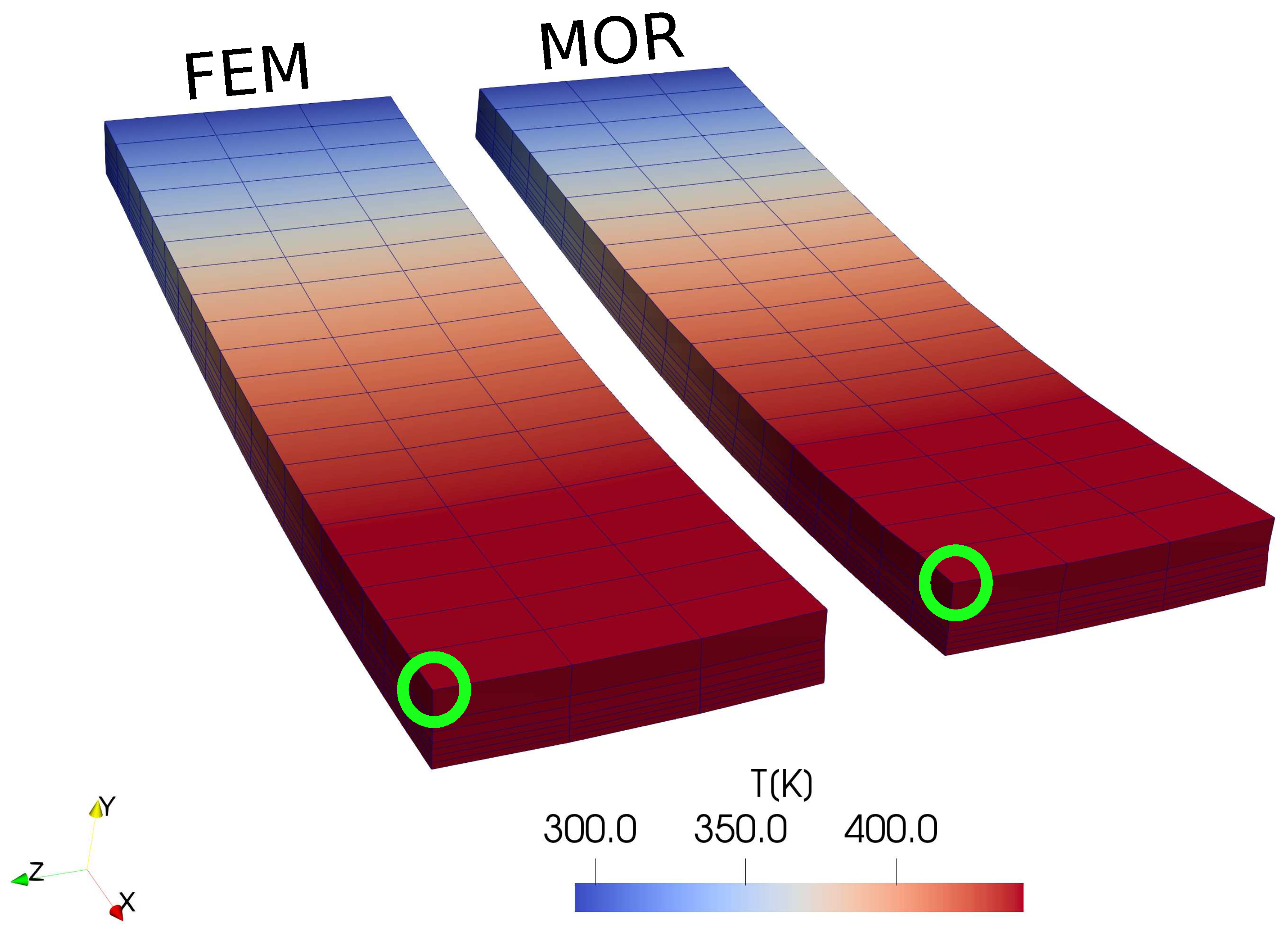
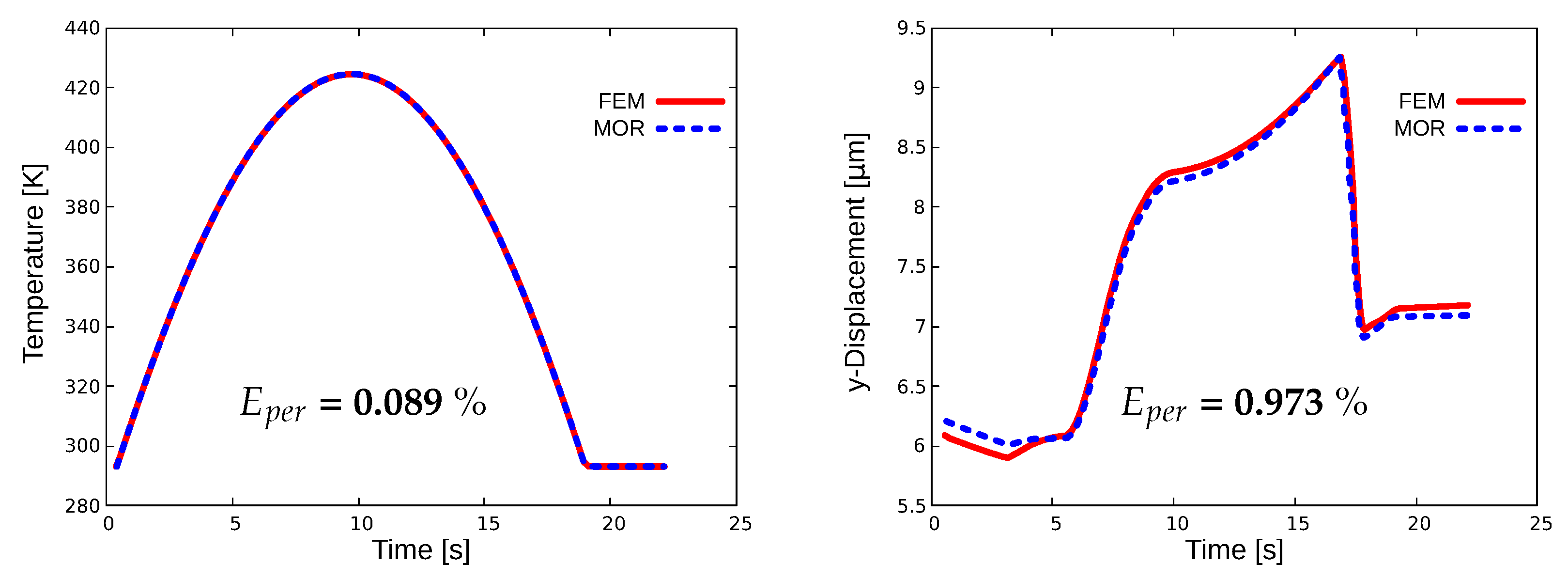
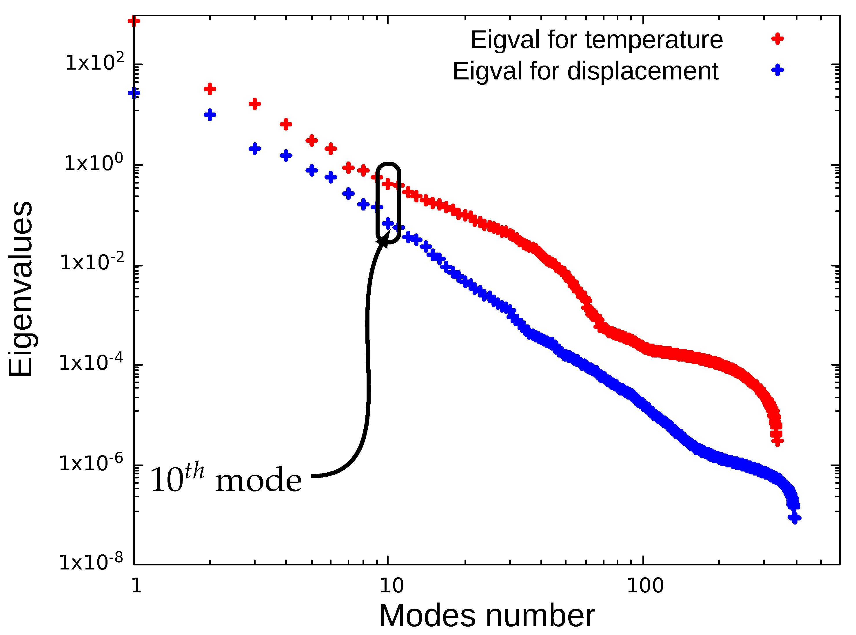
3.1. Single SMA Actuator

We consider here a single actuator for one heat load cycle with appropriate boundary conditions for reduced-order modeling and simulation. For this example, the training data are obtained for different values of Young’s modulus and Poisson’s ratio, replacing the molybdenum layer by solving the full-order model as shown in

Table 1. Parameter data set for training the reduced-order model for beam type trimorph actuator.

Parameter Set	Set 1	Set 2	Set 3
E (MPa)	300	300	300
$\nu$	0.31	0.40	0.49
	Set 4	Set 5	Set 6
E (MPa)	325	325	325
$\nu$	0.31	0.40	0.49
	Set 7	Set 8	Set 9
E (MPa)	350	350	350
$\nu$	0.31	0.40	0.49

. No external force is applied for all the examples, only Joule heating is performed. The snapshots are collected for one heat load cycle. One cycle in which the maximum temperature succeeds the austenite finish temperature ($A_f$) is enough to observe the actuation behavior of our bistable actuator. We acquire 150 snapshots that represent the solution obtained through Equations (16) and (18), respectively. We determine solutions for a wide range of parameter values, as mentioned in Table 1. In total, we collect 1350 snapshots for different material properties. The larger our snapshot matrix, the more accurately we can determine the optimal reduced basis.

POD [34,35,36] is utilized separately to obtain the reduced bases for the displacement and temperature. The model is trained in an offline computation phase. During the online phase, we predict the actuator behavior using any value in the considered parameter range. We minimize the thermomechanical potential (Equation (9)) with respect to the mechanical degrees of freedom to obtain the residual equation for the displacement and, simultaneously, we maximize the same potential with respect to thermal degrees of freedom to obtain the residual equation for the temperature. Then, we obtain the modes which are the global Galerkin ansatz functions for the state variables (displacement and temperature) separately. In this sense, displacements and temperature are comparable and of equal “value” or importance. Moreover, the snapshots calculated from FEM contain nonvanishing Dirichlet boundary conditions for temperature (20 ${}^{\circ }$C), which is technically realized by a homogeneous temperature mode in addition to the other modes, which are normalized by subtracting from all nodes of a given mode the temperature at the clamping position (at $x=0$), such that the modes are zero at that location. In the reduced-order model, temperature Dirichlet boundary conditions are realized, for simplicity, through a penalty approach in the form of a Robin-type boundary condition with very high heat transfer coefficient. The material model developed in [21] was fitted to experimental tensile tests performed at different temperatures and tensile loads. The FEM model predicts reasonable results, and the dependency on the temperature is also captured accurately. Please see Figure 2 in Curtis et al. [46]. In that paper, further experiments with bimorph beam structures similar to the one in this manuscript are also discussed.

We use the following percentage error measure ($E_{per}$) between FEM and MOR

$$E_{per}=\frac{1}{N_{Nd}}\sum _{i=1}^{N_{Nd}}\frac{|{\mathit{u}}_i^{MOR}-{\mathit{u}}_i^{FEM}|}{|{\mathit{u}}_i^{FEM}|}\times 100\%,$$

(20)

where ${\mathit{u}}^{MOR}$ is the displacement solution calculated using MOR, ${\mathit{u}}^{FEM}$ is the displacement solution calculated for FEM and $N_{Nd}$ is the total number of nodes taken for the error calculation. The error measure used for the temperature is defined in analogy. In addition to this global error measure, we use the local measures specified below.

Figure 2 and Figure 3 illustrate the results for FEM and MOR for an “untrained” parameter set, i.e., using values for E and $\nu$, which were not used when computing (see caption of Figure 2) the snapshot matrix. These displacement and temperature graphs are obtained at the left tip of the beam actuator, as marked in the Figure 2 with green circles. We consider 10 and 34 modes for the displacement computations based on the frequency graph of the modes that were obtained after POD computations, as shown in Figure 4. The number of temperature modes taken is equal to the number of displacement modes.

The total time to run the full-scale model for one complete heat cycle and for one parameter value is ∼132 s. Considering the three sets of values for E and $\nu$, this takes ∼1188 s in total to train the MOR against these parameters in an offline stage. After training the MOR against these parameters, the online computations are carried out for an untrained set of parameters. These simulations are carried out on an Intel^® Core™ i7-8850H CPU @ 2.60 GHz with 32 GB RAM. The speedup factors obtained for this example are summarized in

Table 2. Speedup factor for the model considered for one parameter set and one heat load cycle.

CPU Time FEM	Displacement Modes	CPU Time MOR	Speedup	Displacement Error
132 s	10	4.5 s	29.33	2.489%
132 s	34	14.2 s	9.29	0.973%

.

We also carried out the MOR computations for different untrained sets of parameter values ($E=320$ MPa and $\nu =0.38$, $E=330$ MPa and $\nu =0.33$), and the displacement error value is similar for these calculations ($E_{per}=0.98\%,E_{per}=0.971\%$).

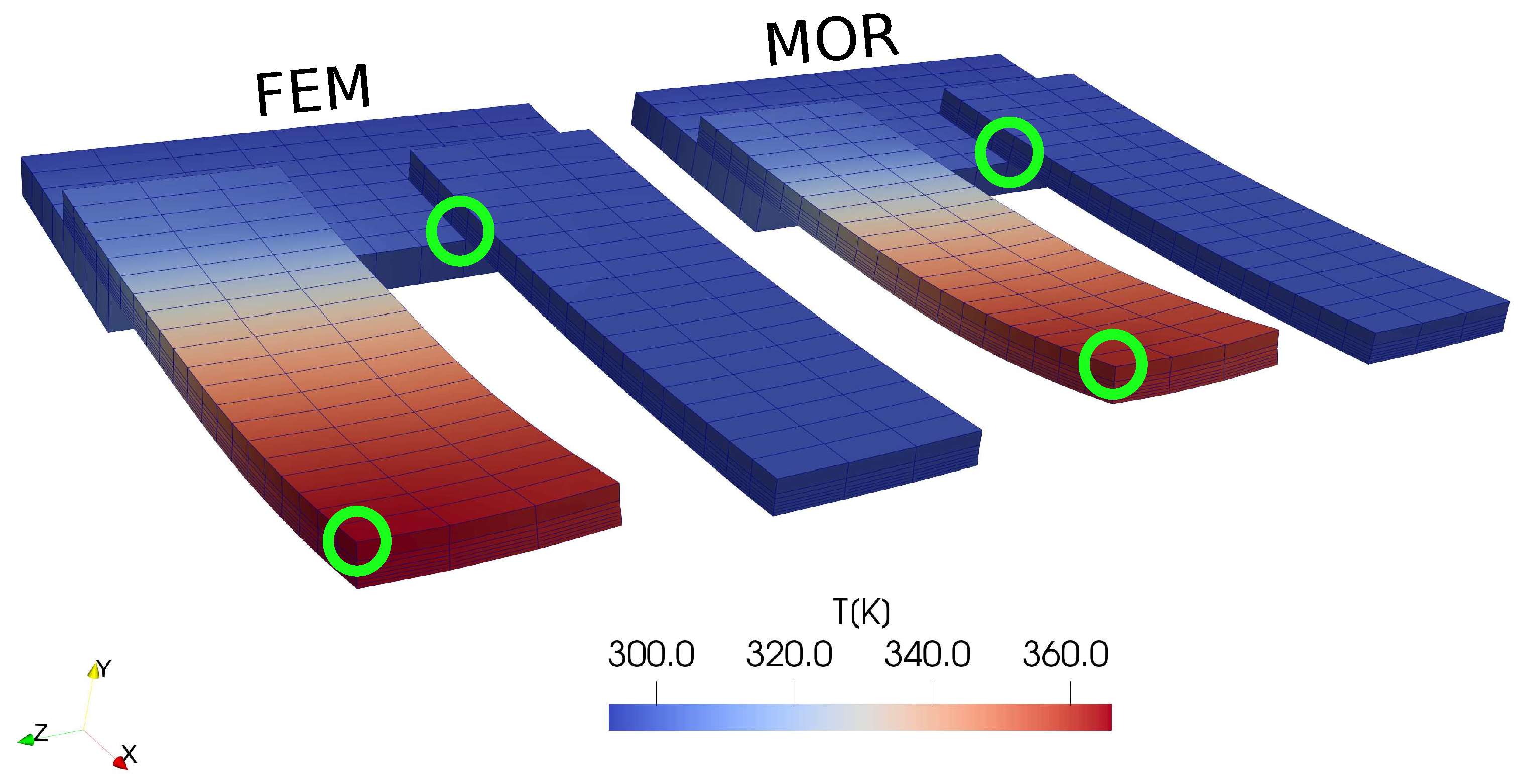
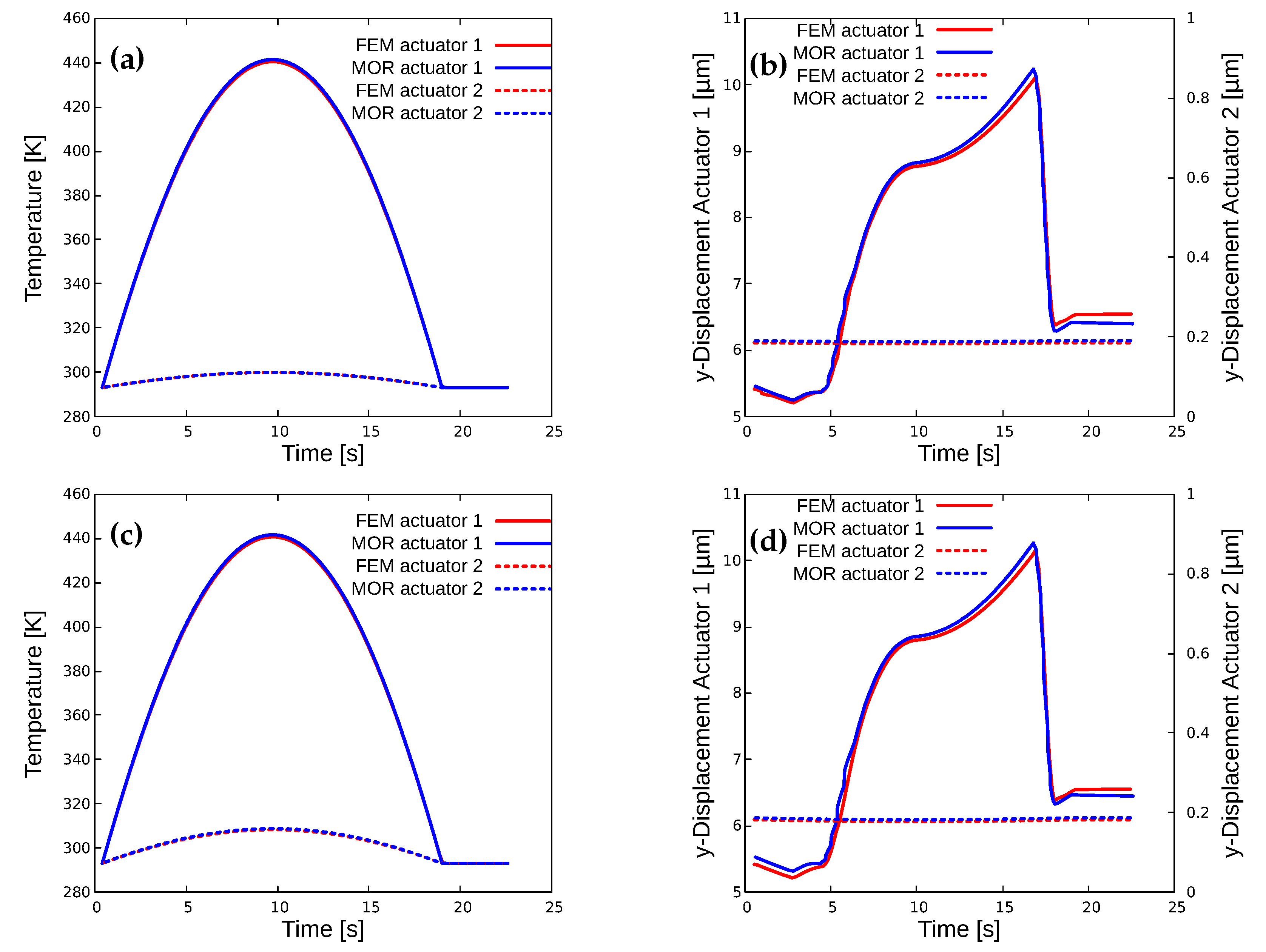
3.2. Cross-Coupling between Actuators

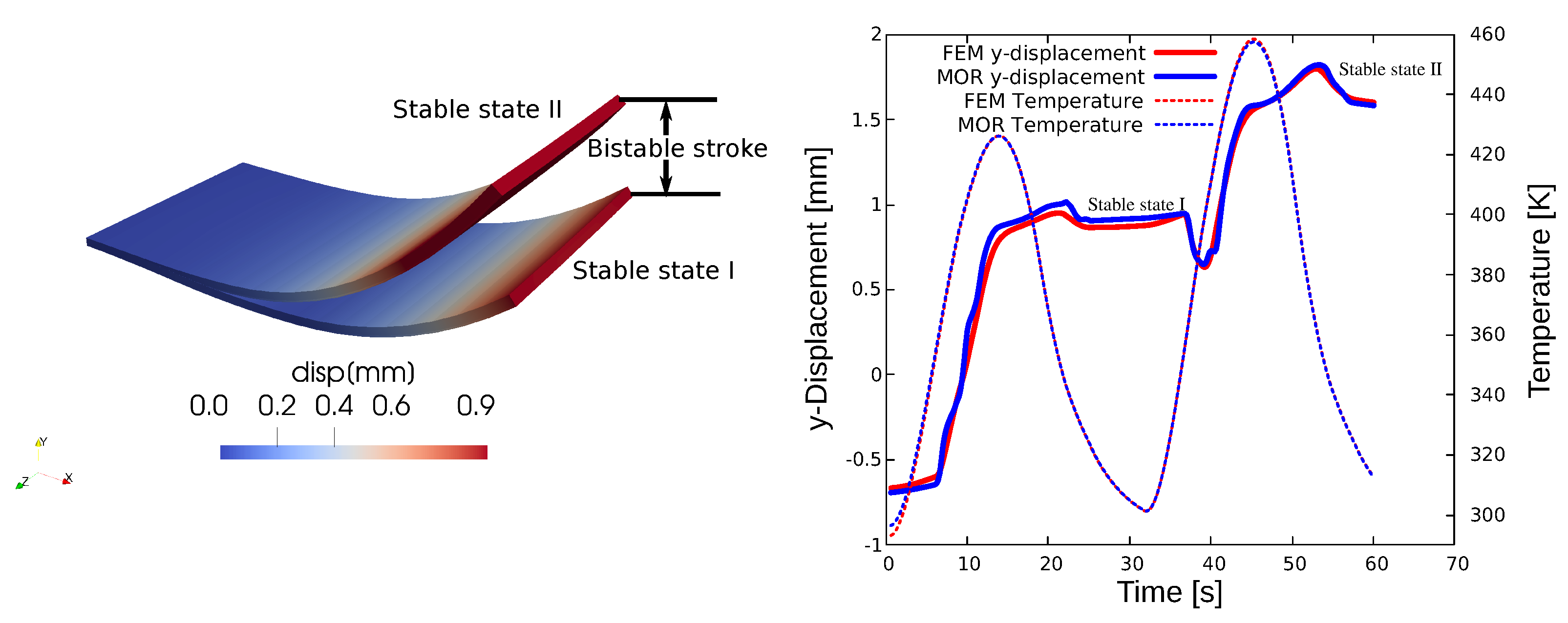
The purpose of this analysis is to comprehend the cross-sensitivities and coupling effects if two actuators cooperate, as well as to investigate the performance of the MOR for a more complicated geometry. In confined spaces, actuating one microactuator that is part of an array might have an influence on the other actuators for cooperative multistable operation. These are unwanted effects that cause a loss of precision in the actuation. For example, if there is a huge cross-coupling between the actuators, activating one actuator through Joule heating will cause the neighboring actuators to actuate, which restricts the design space of the actuator. These cross-coupling effects need to be understood properly [47].

Two actuators are connected at the base to a molybdenum block. The bottom and back-face of the molybdenum base are fixed. A zero Dirichlet boundary condition is applied for the displacement at the fixed locations, and we have a nonzero Dirichlet boundary condition at the back-face of the molybdenum block for temperature, which is 20 ${}^{\circ }$C, and the heat load is applied only at the left actuator. We investigate cross-coupling at different distances d between the actuators using our developed ROM after training the model against different size scales of the actuators. For this case, the snapshots are obtained for the parameters shown in

Table 3. Parameter training data set for cross-coupling effect investigation.

Scale	Dimensions of One Actuator L × W × T	${\mathit{d}}_1$	${\mathit{d}}_2$	${\mathit{d}}_3$
$\mathrm{m}\mathrm{m}$	5 × 1.5 × 0.34	1	0.5	0.1
$\mathsf{\mu }\mathrm{m}$	5 × 1.5 × 0.34	1	0.5	0.1
$\mathrm{n}\mathrm{m}$	500 × 150 × 3.4	100	50	10

. The predictions are given for the untrained case of dimensions, which are 500 × 150 × 24 $\mathsf{\mu }\mathrm{m}$. Figure 5 illustrates the simulation results for the cross-coupling effect due to thermal load application for FEM and MOR.

Figure 6 compares the FEM and MOR results for cross coupling sensitivities. The MOR results generated for this graph are for 52 modes of displacement. The number of temperature modes is taken to be equal to the number of displacement modes. These graphs are obtained for the point at the right tip of the first actuator and the point at the base of second actuator, as illustrated in Figure 5 with green circles. For this analysis, actuating the left actuator has a minor influence on the neighboring actuator, i.e., the sensitivity is not very high. When the temperature reaches 440 K at the left actuator, at a distance of 100 micrometers between the actuators (see Figure 6c), the maximum rise in temperature is 20 K, which is measured at the base of the second actuator, where the maximum temperature is found. This increase in temperature is not enough to initiate the actuation of the second actuator, because the temperature increase in the second actuator has not yet reached $T_g$ of the PMMA and the phase transformation temperature of SMA. The heat is transferred via conduction. The base that connects the two actuators plays an important role as, if we use any material that has a higher conductivity, we may see cross-coupling effects between the actuators.

For the displacement, the error for a small number of modes is large (see

Table 4. Speedup factors for the model considered for one parameter set and one heat load cycle at $d=100\mathsf{\mu }\mathrm{m}$.

CPU Time FEM	Displacement Modes	CPU Time MOR	Speedup	Displacement Error
202 s	10	12.2 s	16.5	6.54%
202 s	52	42 s	4.8	1.29%

). By enriching the basis with more modes, the error decreases. Table 4 summarizes this finding, including the speedup factor for this example.

3.3. Bistability

The term bistability describes the actuator’s ability to be able to hold two stable states at room temperature, which is useful for energy efficient switching of microdevices [48]. We investigate the trimorph NiTiHf/Mo/PMMA-based microactuator’s bistable stroke capabilities using the proposed reduced-order model. The resulting stable states at room temperature are shown in Figure 7. This phenomenon was already discussed in Section 3. Please see, respectively, Sections 4.3 and 3.4 in [21,46] for further details about the bistability phenomenon.

For the bistability performance investigation, we apply two heat load cycles for observing the two stable states of the actuator. We examine the actuator dimensions of 10 × 5 × 0.19 ${\mathrm{m}\mathrm{m}}^3$ with 10, 20 and 160 $\mathsf{\mu }\mathrm{m}$ thicknesses for NiTiHf, Mo and PMMA, respectively.

Figure 7 illustrates the bistability and shows the comparison of FEM and MOR results for displacement and temperature. The first heat cycle heats the actuator just above the polymers glass transition temperature $T_g$ and the second cycle just above the austenite finish temperature of the SMA. The two stable positions at room temperature obtained with the SMA-based actuator are depicted in Figure 7. Here, for the displacement and temperature, using 10 POD modes, the FEM and MOR results agree well. The speedup factor acquired for this analysis is 58.29, with 1061 s and 18.2 s for the FEM and MOR computations, respectively.

4. Conclusions

A reduced-order model for a thermomechanical finite strain shape memory alloy actuator is presented in this paper. Using POD, the reduced basis is obtained. The weak forms of the mechanical and thermal problem are formulated in the reduced-order format. As a major novelty, the reduced-order model is derived from an incremental thermomechanical potential, which ensures a symmetric tangent, and thus allows for efficient solvers and may enable a mathematical model analysis and the employment of enhanced solution methods. The ROM is tested for a single actuator example, cross-coupling effects for two actuators and bistability performance. It was shown from the numerical examples that the model can predict the properties of a parameterized actuator model with controlled accuracy and with less computational effort. The error can be reduced further if the snapshot matrix is enriched with more offline computations.

The ROM developed in this paper still needs further improvement in predicting new parameter values more accurately in less computational time. Therefore, we intend to perform hyper-reduction, in which instead of using each integration point, a reduced set of integration points is evaluated to reduce the computational time.

References

1. Chaudhari, R.; Vora, J.J.; Parikh, D.M. A review on applications of nitinol shape memory alloy. Recent Adv. Mech. Infrastruct. 2021, 123–132. [Google Scholar] [CrossRef]
2. Jani, J.M.; Leary, M.; Subic, A.; Gibson, M.A. A review of shape memory alloy research, applications and opportunities. Mater. Des.-(1980–2015) 2014, 56, 1078–1113. [Google Scholar] [CrossRef]
3. Serry, M.Y.; Moussa, W.A.; Raboud, D.W. Finite-element modeling of shape memory alloy components in smart structures, part II: Application on shape-memory-alloy-embedded smart composite for self-damage control. In Proceedings of the International Conference on MEMS, NANO and Smart Systems, Banff, AB, Canada, 23–23 July 2003; pp. 423–429. [Google Scholar]
4. Shibly, H.; Söffker, D. Mathematical models of shape memory alloy behavior for online and fast prediction of the hysteretic behavior. Nonlinear Dyn. 2010, 62, 53–66. [Google Scholar] [CrossRef]
5. Liang, C.; Rogers, C.A. One-dimensional thermomechanical constitutive relations for shape memory materials. J. Intell. Mater. Syst. Struct. 1997, 8, 285–302. [Google Scholar] [CrossRef]
6. Oka, S.; Saito, S.; Onodera, R. Mathematical Model of Shape Memory Alloy Actuator for Resistance Control System. In Proceedings of the 2021 International Conference on Advanced Mechatronic Systems (ICAMechS), Tokyo, Japan, 9–12 December 2021; pp. 7–11. [Google Scholar]
7. Huang, W. On the selection of shape memory alloys for actuators. Mater. Des. 2002, 23, 11–19. [Google Scholar] [CrossRef]
8. AbuZaiter, A.; Nafea, M.; Mohd Faudzi, A.A.; Kazi, S.; Mohamed Ali, M.S. Thermomechanical behavior of bulk NiTi shape-memory-alloy microactuators based on bimorph actuation. Microsyst. Technol. 2016, 22, 2125–2131. [Google Scholar] [CrossRef]
9. Terriault, P.; Brailovski, V. Modeling of shape memory alloy actuators using Likhachev’s formulation. J. Intell. Mater. Syst. Struct. 2011, 22, 353–368. [Google Scholar] [CrossRef]
10. Lagoudas, D.C.; Miller, D.A.; Rong, L.; Kumar, P.K. Thermomechanical fatigue of shape memory alloys. Smart Materials and Structures. 2009, 18, 085021. [Google Scholar] [CrossRef]
11. Song, S.H.; Lee, J.Y.; Rodrigue, H.; Choi, I.S.; Kang, Y.J.; Ahn, S.H. 35 Hz shape memory alloy actuator with bending-twisting mode. Sci. Rep. 2016, 6, 1–3. [Google Scholar] [CrossRef] [PubMed] [Green Version]
12. Stachiv, I.; Gan, L. Hybrid shape memory alloy-based nanomechanical resonators for ultrathin film elastic properties determination and heavy mass spectrometry. Materials 2019, 12, 3593. [Google Scholar] [CrossRef] [PubMed]
13. Samal, S.; Kosjakova, O.; Vokoun, D.; Stachiv, I. Shape Memory Behaviour of PMMA-Coated NiTi Alloy under Thermal Cycle. Polymers 2022, 14, 2932. [Google Scholar] [CrossRef] [PubMed]
14. Winzek, B.; Schmitz, S.; Rumpf, H.; Sterzl, T.; Hassdorf, R.; Thienhaus, S.; Feydt, J.; Moske, M.; Quandt, E. Recent developments in shape memory thin film technology. Mater. Sci. Eng. A 2004, 378, 40–46. [Google Scholar] [CrossRef]
15. Machairas, T.T.; Solomou, A.G.; Karakalas, A.A.; Saravanos, D.A. Effect of shape memory alloy actuator geometric non-linearity and thermomechanical coupling on the response of morphing structures. J. Intell. Mater. Syst. Struct. 2019, 30, 2166–2185. [Google Scholar] [CrossRef]
16. Chang, B.C.; Shaw, J.A.; Iadicola, M.A. Thermodynamics of shape memory alloy wire: Modeling, experiments, and application. Contin. Mech. Thermodyn. 2006, 18, 83–118. [Google Scholar] [CrossRef]
17. Roh, J.H.; Han, J.H.; Lee, I. Nonlinear finite element simulation of shape adaptive structures with SMA strip actuator. J. Intell. Mater. Syst. Struct. 2006, 17, 1007–1022. [Google Scholar] [CrossRef]
18. Popov, P.; Lagoudas, D.C. A 3-D constitutive model for shape memory alloys incorporating pseudoelasticity and detwinning of self-accommodated martensite. Int. J. Plast. 2007, 23, 1679–1720. [Google Scholar] [CrossRef]
19. Yang, Q.; Stainier, L.; Ortiz, M. A variational formulation of the coupled thermo-mechanical boundary-value problem for general dissipative solids. J. Mech. Phys. Solids 2006, 54, 401–424. [Google Scholar] [CrossRef]
20. Saleeb, A.F.; Dhakal, B.; Hosseini, M.S.; Padula, S.A., II. Large scale simulation of NiTi helical spring actuators under repeated thermomechanical cycles. Smart Mater. Struct. 2013, 22, 094006. [Google Scholar] [CrossRef] [Green Version]
21. Sielenkämper, M.; Wulfinghoff, S. A thermomechanical finite strain shape memory alloy model and its application to bistable actuators. Acta Mech. 2022, 233, 3059–3094. [Google Scholar] [CrossRef]
22. Sedlak, P.; Frost, M.; Benešová, B.; Zineb, T.B.; Šittner, P. Thermomechanical model for NiTi-based shape memory alloys including R-phase and material anisotropy under multi-axial loadings. Int. J. Plast. 2012, 39, 132–151. [Google Scholar] [CrossRef]
23. Potapov, P.L.; Shelyakov, A.V.; Gulyaev, A.A.; Svistunov, E.L.; Matveeva, N.M.; Hodgson, D. Effect of Hf on the structure of Ni-Ti martensitic alloys. Mater. Lett. 1997, 32, 247–250. [Google Scholar] [CrossRef]
24. Frost, M.; Benešová, B.; Seiner, H.; Kružík, M.; Šittner, P.; Sedlák, P. Thermomechanical model for NiTi-based shape memory alloys covering macroscopic localization of martensitic transformation. Int. J. Solids Struct. 2021, 221, 117–129. [Google Scholar] [CrossRef]
25. Solomou, A.G.; Machairas, T.T.; Saravanos, D.A. A coupled thermomechanical beam finite element for the simulation of shape memory alloy actuators. J. Intell. Mater. Syst. Struct. 2014, 25, 890–907. [Google Scholar] [CrossRef]
26. Shah, N.V.; Girfoglio, M.; Quintela, P.; Rozza, G.; Lengomin, A.; Ballarin, F.; Barral, P. Finite element based Model Order Reduction for parametrized one-way coupled steady state linear thermo-mechanical problems. Finite Elem. Anal. Des. 2022, 212, 103837. [Google Scholar] [CrossRef]
27. Chemisky, Y.; Duval, A.; Patoor, E.; Zineb, T.B. Constitutive model for shape memory alloys including phase transformation, martensitic reorientation and twins accommodation. Mech. Mater. 2011, 43, 361–376. [Google Scholar] [CrossRef]
28. Merzouki, T.; Duval, A.; Zineb, T.B. Finite element analysis of a shape memory alloy actuator for a micropump. Simul. Model. Pract. Theory 2012, 27, 112–126. [Google Scholar] [CrossRef]
29. Hickey, D.; Hoffait, S.; Rothkegel, J.; Kerschen, G.; Brüls, O. Model Order Reduction Techniques for Thermomechanical Systems with Nonlinear Radiative Heat Transfer Using Proper Order Decomposition. Available online: https://www.semanticscholar.org/paper/Model-order-reduction-techniques-for-systems-with-Hickey-Hoffait/09ff384c345b140035ac20271f4ec9fbf07ac503 (accessed on 10 October 2022).
30. Hickey, D.; Masset, L.; Kerschen, G.; Brüls, O. Proper orthogonal decomposition for nonlinear radiative heat transfer problems. In Proceedings of the International Design Engineering Technical Conferences and Computers and Information in Engineering Conference, Washington, DC, USA, 28–31 August 2011; Volume 54785, pp. 407–418. [Google Scholar]
31. Binion, D.; Chen, X. A Krylov enhanced proper orthogonal decomposition method for efficient nonlinear model reduction. Finite Elem. Anal. Des. 2011, 47, 728–738. [Google Scholar] [CrossRef]
32. Choi, Y.; Carlberg, K. Space-time least-squares Petrov–Galerkin projection for nonlinear model reduction. SIAM J. Sci. Comput. 2019, 41, A26–A58. [Google Scholar] [CrossRef] [Green Version]
33. Guo, M.; Hesthaven, J.S. Reduced order modeling for nonlinear structural analysis using Gaussian process regression. Comput. Methods Appl. Mech. Eng. 2018, 341, 807–826. [Google Scholar] [CrossRef]
34. Lin, W.Z.; Lee, K.H.; Lim, S.P.; Liang, Y.C. Proper orthogonal decomposition and component mode synthesis in macromodel generation for the dynamic simulation of a complex MEMS device. J. Micromech. Microeng. 2003, 13, 646. [Google Scholar] [CrossRef]
35. Kerschen, G.; Golinval, J.C.; Vakakis, A.F.; Bergman, L.A. The method of proper orthogonal decomposition for dynamical characterization and order reduction of mechanical systems: An overview. Nonlinear Dyn. 2005, 41, 147–169. [Google Scholar] [CrossRef]
36. Friderikos, O.; Olive, M.; Baranger, E.; Sagris, D.; David, C. A Space-Time POD Basis Interpolation on Grassmann Manifolds for Parametric Simulations of Rigid-Viscoplastic FEM. MATEC WEB Conf. 2020, 318, 01043. [Google Scholar] [CrossRef]
37. Vettermann, J.; Steinert, A.; Brecher, C.; Benner, P.; Saak, J. Compact thermo-mechanical models for the fast simulation of machine tools with nonlinear component behavior. at-Automatisierungstechnik 2022, 70, 692–704. [Google Scholar] [CrossRef]
38. Umunnakwe, C.B.; Zawra, I.; Yuan, C.; Rudnyi, E.B.; Hohlfeld, D.; Niessner, M.; Bechtold, T. Model Order Reduction of a Thermo-Mechanical Packaged Chip Model for automotive MOSFET applications. In Proceedings of the 2022 23rd International Conference on Thermal, Mechanical and Multi-Physics Simulation and Experiments in Microelectronics and Microsystems (EuroSimE), St Julian, Malta, 25–27 April 2022; pp. 1–5. [Google Scholar]
39. Hu, J.; Zhang, B.; Gao, X. Reduced order model analysis method via proper orthogonal decomposition for transient heat conduction. Sci. Sin. Phys. Mech. Astron. 2015, 45, 14602. [Google Scholar] [CrossRef] [Green Version]
40. Jia, W.; Helenbrook, B.T.; Cheng, M.C. A reduced order thermal model with application to multi-fin field effect transistor structure. In Proceedings of the Fourteenth Intersociety Conference on Thermal and Thermomechanical Phenomena in Electronic Systems (ITherm), Orlando, FL, USA, 27–30 May 2014; pp. 1–8. [Google Scholar]
41. Bikcora, C.; Weiland, S.; Coene, W.M. Thermal deformation prediction in reticles for extreme ultraviolet lithography based on a measurement-dependent low-order model. IEEE Trans. Semicond. Manuf. 2014, 27, 104–117. [Google Scholar] [CrossRef]
42. Hernández-Becerro, P.; Spescha, D.; Wegener, K. Model order reduction of thermo-mechanical models with parametric convective boundary conditions: Focus on machine tools. Comput. Mech. 2021, 67, 167–184. [Google Scholar] [CrossRef]
43. Das, A.; Khoury, A.; Divo, E.; Huayamave, V.; Ceballos, A.; Eaglin, R.; Kassab, A.; Payne, A.; Yelundur, V.; Seigneur, H. Real-time thermomechanical modeling of PV cell fabrication via a pod-trained RBF interpolation network. Comput. Model. Eng. Sci. 2020, 122, 757–777. [Google Scholar] [CrossRef]
44. Taylor, R.L.; Govindjee, S. FEAP-A Finite Element Analysis Program, Programmer Manual: v8. 6; University of California: Berkeley, CA, USA, 2022; Available online: http://projects.ce.berkeley.edu/feap/ (accessed on 25 October 2022).
45. Ahrens, J.; Geveci, B.; Law, C. Paraview: An end-user tool for large data visualization. Vis. Handb. 2005, 717. [Google Scholar]
46. Curtis, S.M.; Sielenkämper, M.; Arivanandhan, G.; Dengiz, D.; Li, Z.; Jetter, J.; Hanke, L.; Bumke, L.; Quandt, E.; Wulfinghoff, S.; et al. TiNiHf/SiO2/Si shape memory film composites for bi-directional micro actuation. Int. J. Smart Nano Mater. 2022, 13, 1–22. [Google Scholar] [CrossRef]
47. Habineza, D.; Zouari, M.; Le Gorrec, Y.; Rakotondrabe, M. Multivariable compensation of hysteresis, creep, badly damped vibration, and cross couplings in multiaxes piezoelectric actuators. IEEE Trans. Autom. Sci. Eng. 2017, 15, 1639–1653. [Google Scholar] [CrossRef] [Green Version]
48. Barth, J.; Krevet, B.; Kohl, M. A bistable shape memory microswitch with high energy density. Smart Mater. Struct. 2010, 19, 094004. [Google Scholar] [CrossRef]
Figure 1. Dimensions of the actuator assembly, which is clamped at the left side. The red layer is polymer, blue is SMA and gray is molybdenum.
Actuators 12 00036 g001
Figure 2. FEM and MOR result comparison for temperature for an “untrained” parameter set with 10 modes ( E = 331 MPa and ν = 0.35 ).
Actuators 12 00036 g002
Figure 3. FEM and MOR comparison for displacement and temperature for one heat cycle (left). Temperature graph with 10 modes. Displacement graph with 34 modes (right).
Actuators 12 00036 g003
Figure 4. Eigenvalue graph for modes obtained after POD computation for the displacement and temperature.
Actuators 12 00036 g004
Figure 5. FEM and MOR temperature results for cross-coupling effect investigation for an untrained actuator geometry (500 × 150 × 24 μ m ).
Actuators 12 00036 g005
Figure 6. Temperature and displacement graphs for different distances between actuators for the investigation of cross-coupling effects: (a) Temperature prediction at d = 1000 μ m . (b) Displacement prediction at d = 1000 μ m . (c) Temperature prediction at d = 100 μ m . (d) Displacement prediction at d = 100 μ m .
Actuators 12 00036 g006
Figure 7. MOR results for displacement magnitude at two different stable states (left): Bistable positions for the selected actuator with FEM and MOR comparison (right).
Actuators 12 00036 g007