Research on Control Strategy of Heavy-Haul Train on Long and Steep Downgrades

Abstract

The control of heavy-haul trains has always been the focus of China’s railway transportation development. One key challenge is the coordination of electric braking and air braking control when the electric-air combined braking is applied on long and steep downgrades. This is normally reliant on manual driving and thus is not cost-effective. To improve the safety and efficiency of train operation in existing heavy-haul railway lines, a multi-label random forest (ML-RF) based approach for heavy-haul train (HHT) operation is proposed. The control characteristics of electric braking and air braking on long and steep downgrades are analyzed first. A prediction model of control strategy is then established with the combination of line conditions and definition of multi-label learning. To evaluate the performance of the model, the 10-fold cross-validation method is adopted. Furthermore, a model parameter optimization algorithm based on evaluation metrics is designed. The feasibility of the proposed approach is demonstrated by the testing results on the actual train running data of one railway line.

1. Introduction

Heavy-haul transportation plays a vital role in improving transportation efficiency, increasing economic profits, and reducing the costs of logistics transportation. It is also one of the main directions of railway freight development in China, the United States, Brazil, Australia, South Africa, and so on [1,2]. Due to the large weight, long grouping, increasing traction mass, and complex line conditions, the control of heavy-haul trains (HHTs) is facing great challenges [3]. Typically in China, the characteristics of vehicles, lines, locomotive control, and operation are as follows:

• On the railway lines which transport coal from west to east in China, the maximum load capacity of the train has reached 20,000 tons, with a total length of about 2.6 km, and the number of vehicles is more than 200.
• There are many sections with long and steep downgrades, and the value of the slope reaches 12‰. Since “long and steep downgrades” is a relative concept, a unified definition should be given for trains with different electric braking capacities [4], which is shown in Equation (1).
• When the HHT runs on long and steep downgrades, the speed will increase continuously. To avoid exceeding the speed limit, the electric braking and air braking should be used together, which is called “electric-air combined braking” [5,6]. However, if air braking is applied for a long period, the shortage of air-filled time may become a serious problem. This may lead to insufficient force to reduce the speed in the next braking. Therefore, the air braking must be applied intermittently for HHTs, and the driver must choose the timing of the braking application and release accurately until the train leaves the given sections [7]. At the same time, the use of electric braking prevents the train speed from increasing sharply, and makes the air-filled time of the train pipe more sufficient. This contributes to improving the release performance of the train.
• The heavy-haul railway line is long, represented by the Datong-Qinhuangdao railway and the Shuozhou-Huanghua railway, the lengths of which are about 653 km and 594 km, respectively. Importantly, HHTs barely stop in between stations, and thus drivers usually suffer from higher work intensities [8].

Under the manual driving mode, the above-mentioned characteristics challenge the drivers on the control of HHTs in terms of both mature skills and good psychological and physical qualities. Generally, in addition to systematic theoretical training, new drivers need to take part in a lot of practice to gain enough experience to become competent in this field. This is considered to be time-consuming. Secondly, even for the competent drivers, some accidents could happen due to tiredness after tedious operations. As some works have shown [9,10], when the line condition and braking system are determined, improper control of the locomotive, including the timing and control force, will increase the longitudinal force of the train and even cause accidents such as coupler broken. Therefore, to reduce the cost of training drivers and to increase safety and efficiency, it is necessary and significant to develop an intelligent control strategy of HHTs.

In recent years, attention has been paid to the control of HHTs in academia. He and Zhang [11] presented a braking control method based on factor analysis, including braking frequency, pressure reduction, initial braking speed, and release speed. Dong and Wei [12] used the simulation system of longitudinal dynamics to optimize the control of braking, and pointed out that the number of braking can be reduced by changing the initial braking speed, braking current and air braking time. Zhang et al. [13] put forward an air braking application method for the operation of 23,000 t HHT, with a 30 t axle load, on long and steep downgrades. To reduce the longitudinal impulse caused by the braking delay of HHTs, a braking control strategy was given in [14]. Yang et al. [4] designed a simulation method based on the train control requirements and principles to provide the running speed curve faster. Considering the characteristics of air braking application and release constraints, a periodic braking strategy of “full braking, full electric braking, full braking” based on the maximum principle was proposed in [15]. The control strategy of air braking was studied by using heuristic algorithms in [16,17], mixed-integer linear programming in [18] and the dynamic programming method in [19]. On the other hand, with the wide application of machine learning, the advantage of the traction and braking of HHT as a non-linear process is becoming more and more prominent. The application of machine learning on HHT control has also attracted more and more attention. Wang et al. [20] introduced a strategy generation method based on machine learning to solve the problem of air braking control. Huang et al. [21] proposed a method based on neural networks for pressure reduction and release time prediction. Wei et al. [22] introduced the Adaboost based model and achieved the intelligent control of air braking for HHTs. Tang et al. [23] proposed a reinforcement learning method based on the traction and electric braking characteristics of electric locomotives and discussed the influences of slope and speed limit on control. Bai et al. [24] proposed a fuzzy neural network based on the historical data of train stopping to obtain the initial braking position under the given braking ratio, line conditions and initial braking speed.

It can be observed that most existing studies mainly consider the characteristics of air braking control, and have not taken the coordination of air braking and electric braking control into consideration. Accordingly, we carry out this study. The main contributions of the research are summarized as follows:

• The control problem of HHT on long and steep downgrades is transformed into a multi-label learning process.
• The research method based on multi-label random forest (ML-RF) is proposed, in combination with line conditions, running speed, and other factors. Because ML-RF belongs to the category of machine learning, the control strategy can be obtained without the need of an accurate train model.
• With evaluation metrics of multi-label learning, a parameter optimization algorithm for ML-RF is designed. Tests are also conducted, considering the neutral zone.

The rest of this paper is organized as follows. Section 2 presents the mathematical formulation of the studied problem. In Section 3, a multi-label prediction framework is proposed. In Section 4, the optimal parameters are calculated and performance testing is conducted. In Section 5, conclusions are given.

2. Problem Description

A long and steep downgrades section is shown in Figure 1, which consists of three parts, with values of i₁‰, i₂‰ and i₃‰, lengths of L₁, L₂ and L₃ respectively, and one neutral zone marked “F” contained. x₀ and x₁ are the beginning and end position of the neutral zone.

When trains running on such lines, if only the electric braking is applied, we have,

$$\left(-F_{\mathrm{e}}^{\max }-F_{\mathrm{r}}\right)>0\cup \left(v_{L_{\mathrm{r}}}>v_{\lim },0<L_{\mathrm{r}}<\left(L_1+L_2+L_3\right)\right)$$

(1)

where $F_{\mathrm{e}}^{\max }$ denotes the maximum instantaneous electric braking force, which is related to the type of locomotive; $F_{\mathrm{r}}$ denotes the running resistance, with the basic resistance, slope resistance, curve resistance, and tunnel resistance included; $v_{\lim }$ is the speed limit depending on the railway line or the temporary configuration during operation; $v_{L_{\mathrm{r}}}$ is the speed related to the running distance $L_{\mathrm{r}}$.

So, for a non-neutral zone, the dynamics description is given as follows:

$$F=-F_{\mathrm{e}}-F_{\mathrm{a}}-F_{\mathrm{r}},\left(x<x_0\right)\cup \left(x>x_1\right)$$

(2)

where $F$ is the resultant force, $F_{\mathrm{e}}$ is the electric braking force, $F_{\mathrm{a}}$ is the air braking force, and x is the train position.

While for the neutral zone in the electric railway, the output of electric braking force is equal to zero, and the air braking force is applied during the trip, the dynamics description is given as follows:

$$F=-F_{\mathrm{a}}-F_{\mathrm{r}}, x_0\le x\le x_1$$

(3)

When the neutral zone is located on long and steep downgrades, the train needs to output air brake force for speed regulation. The timing of air braking application is very important. If it is applied too early, the train may stop in the neutral zone due to the low speed. If it is applied too late, the train may run over the speed limit. Therefore, it should be applied at an appropriate time, according to the train running speed, the length of the neutral zone and the output value of electric braking force in order to ensure the smooth running of the train in this section.

In fact, during the actual operation, the output of the electric braking force is reduced to zero in advance, and recovered to a certain notch with delay, i.e., these differences are measured by the distance l₀ and l₁, Equations (2) and (3) can be rewritten as follows:

$$\begin{array}{c}F=-F_{\mathrm{e}}-F_{\mathrm{a}}-F_{\mathrm{r}},\left(x<x_0-l_0\right)\cup \left(x>x_1+l_1\right)\\ F=-F_{\mathrm{a}}-F_{\mathrm{r}},x_0-l_0\le x\le x_1+l_1\end{array}$$

(4)

In this paper, the problem of braking control for HHTs is studied from two aspects according to the operation rules. Application or release, and pressure reduction are obtained, which is called air braking force prediction. On the other hand, application or no application, and notches are obtained, which is called electric braking force prediction. Here, the multi-label classification method is used to predict them at the same time, and then the relation between air braking and electric braking is analyzed.

The problem can be described as follows:

$$\mathrm{function} f:\chi \to y$$

(5)

where $\chi$ denotes the input space, and objects are represented as feature vectors from $\chi$; $y$ denotes the output space, and labels come from the set L that spans y, referring to the application or release and pressure reduction of air braking and the application (notches) or no application of electric braking.

The single-label classification refers to the fact that an object can only be marked by one label l in sets L with multiple independent labels, $\left|L\right|>1$. If $\left|L\right|=2$, it is a two-class classification problem with single-label. If $\left|L\right|>2$, it is a multi-class classification with single-label. Multi-label classification means that an object can be marked by a group of labels $y_{\mathrm{l}}\subseteq L$, and labels are generally not independent.

Combined with the definition of multi-label learning, $y$ can be written as follows:

$$y=\left\{l_{\mathrm{e}},l_{\mathrm{a}}\right\}$$

(6)

where l_e and l_a are the labels corresponding to electric braking and air braking.

3. Prediction Model of Control Strategy

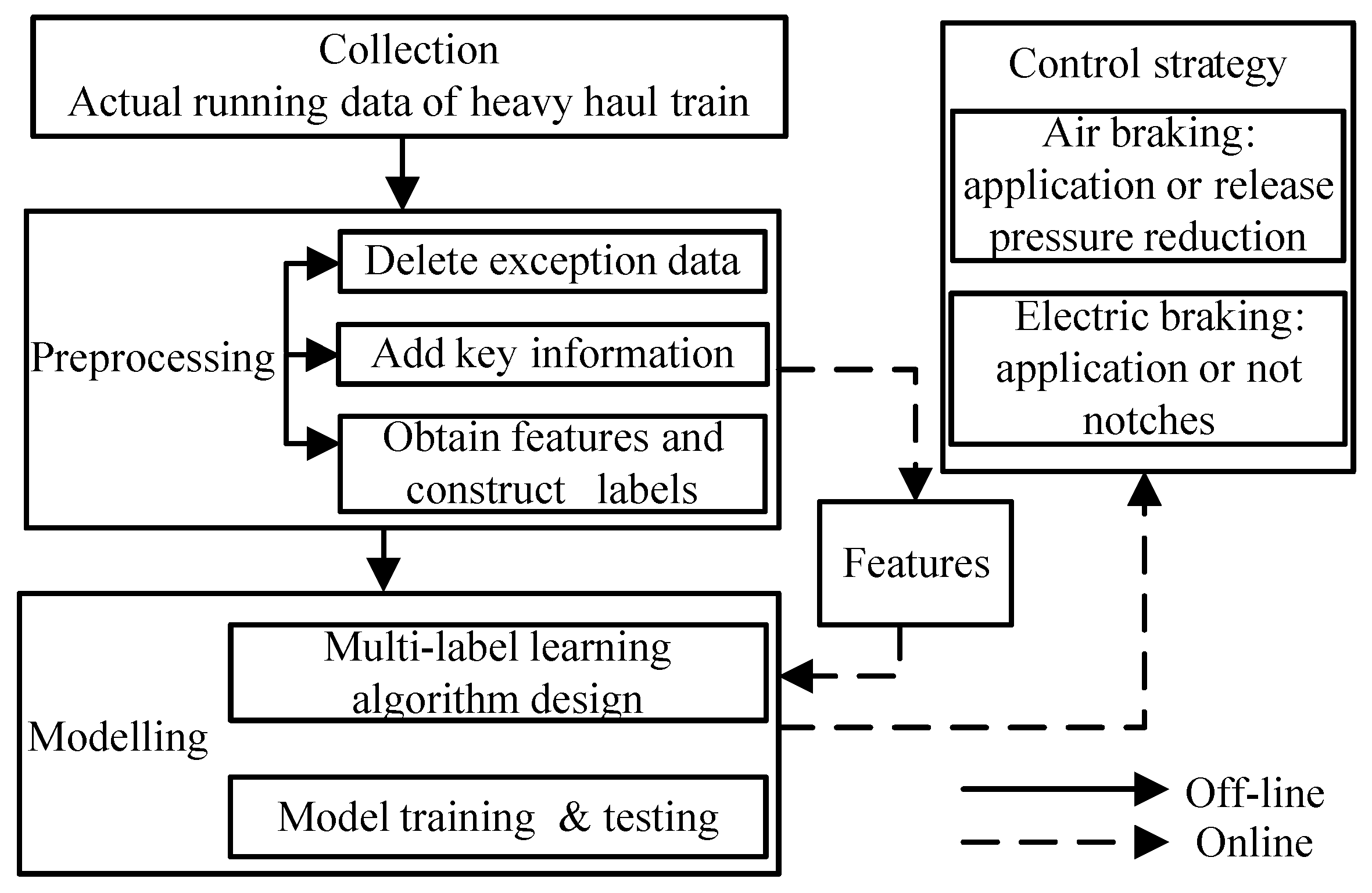
As is shown in Figure 2, we describe the framework of control strategy prediction for HHTs. First, collect the train running data. Then, make the information more consistent with the modelling requirements through data preprocessing. Furthermore, the multi-label learning algorithm is put forward to train a model. Finally, some data is used to test and analyze the model. When all of these are done, we will get the prediction model, which could be applied to a train operation simulation.

With regard to actual running data, it is important to note that,

• The train operation status and the control process of the driver are reflected in the data.
• The train operation status is the result of forces acting on the real train. Here, the resistance forces and braking forces are included.
• For a driver, longitudinal train dynamics and braking system characteristics are considered during driving, such as the air-filled time.

3.1. Data Preprocessing

After processing the exception data and adding some information, the features are determined, including the kilometer post, running speed, speed limit, signaling, train pipe pressure, equalizing cylinder pressure, slope information at the current location, slope and neutral zone information on the front of the train within a certain distance, etc.

Remark 1. 

For the control of air braking, the pressure reduction usually varies from 50 kPa to 140 kPa at 10 kPa intervals. When the train runs on long and steep downgrades, the pressure reduction of 50 kPa could make the HHT slow down; here, the normal stopping and stopping caused by improper control are not considered. The binary variable is then introduced to indicate the trigger timing of the application and release of air braking.

Remark 2. 

For the control of electric braking, the force is reflected by the notch information. In this paper, the application is assumed to have five notches.

Based on the assumptions, data collection is done according to the pressure reduction, and the electric braking force is discretized according to the total number of notches. The labels can be defined as follows:

$$l_{\mathrm{e}}=\{\begin{array}{l}0\hspace{1em}\hspace{1em}I/I_{\mathrm{z}}=0 \\ 1\hspace{1em} 0< I/I_{\mathrm{z}}\le 0.2\\ 2\hspace{1em}0.2< I/I_{\mathrm{z}}\le 0.4\\ 3\hspace{1em} 0.4< I/I_{\mathrm{z}}\le 0.6\\ 4\hspace{1em} 0.6< I/I_{\mathrm{z}}\le 0.8\\ 5\hspace{1em} 0.8< I/I_{\mathrm{z}}\le 1.0\end{array}$$

(7)

$$l_{\mathrm{a}}=\{\begin{array}{l}0\\ 1\end{array}$$

(8)

where I is the instantaneous braking current, I_z is the rated braking current. l_e = 0, electric braking is not applied; l_e > 0, electric braking is applied. l_a = 0, air braking is released; l_a = 1, air braking is applied. l_a = 0 → l_a = 1: the application timing of air braking; l_a = 1 → l_a = 0: the release timing of air braking. In actual operation, the label values correspond to three cases from regimes of a train, as shown below:

• l_e > 0, l_a = 0: electric braking is applied, while air braking is released;
• l_e > 0, l_a = 1: electric braking and air braking are applied together;
• l_e = 0, l_a = 1: only air braking is applied, especially when the train is running through a neutral zone.

Then, when l_e and l_a are obtained, the braking force can be calculated by:

$$F_{\mathrm{e}}=F_{\mathrm{e}}^{\max }\frac{I}{I_{\mathrm{z}}}\rho$$

(9)

$$F_{\mathrm{a}}=f\left(l_{\mathrm{a}},v,p,t\right)$$

(10)

where $\rho$ is the correction factor; v is the train speed; p is the pressure reduction; when t = 0, the locomotive receives the command of application or release.

3.2. Multi-Label Learning Algorithm Based on Random Forest

A multi-label learning task [25] means to learn a function that can predict a set of labels for an object which is matched to the control characteristics of HHTs.

Random forest (RF), known as one of the best classification algorithms, has three characteristics [26]: it performs well on most data sets and has great advantages over other algorithms; it performs well when dealing with high-dimensional data; it is not needed to select features in advance, and important feature sets are given in the process of training. In addition, the prediction and training speed of RF is greatly improved with a parallel process. Therefore, RF is selected as the basic algorithm in this paper.

RF is a typical ensemble learning model that uses bootstrap aggregation. As the name suggests, RF is a method of constructing decision forest randomly, and its randomness or the diversity of trees is mainly reflected in the randomization of training data set and input variable set [27]. Therefore, RF avoids the appearance of over fitting and has good ability with regard to anti-noise.

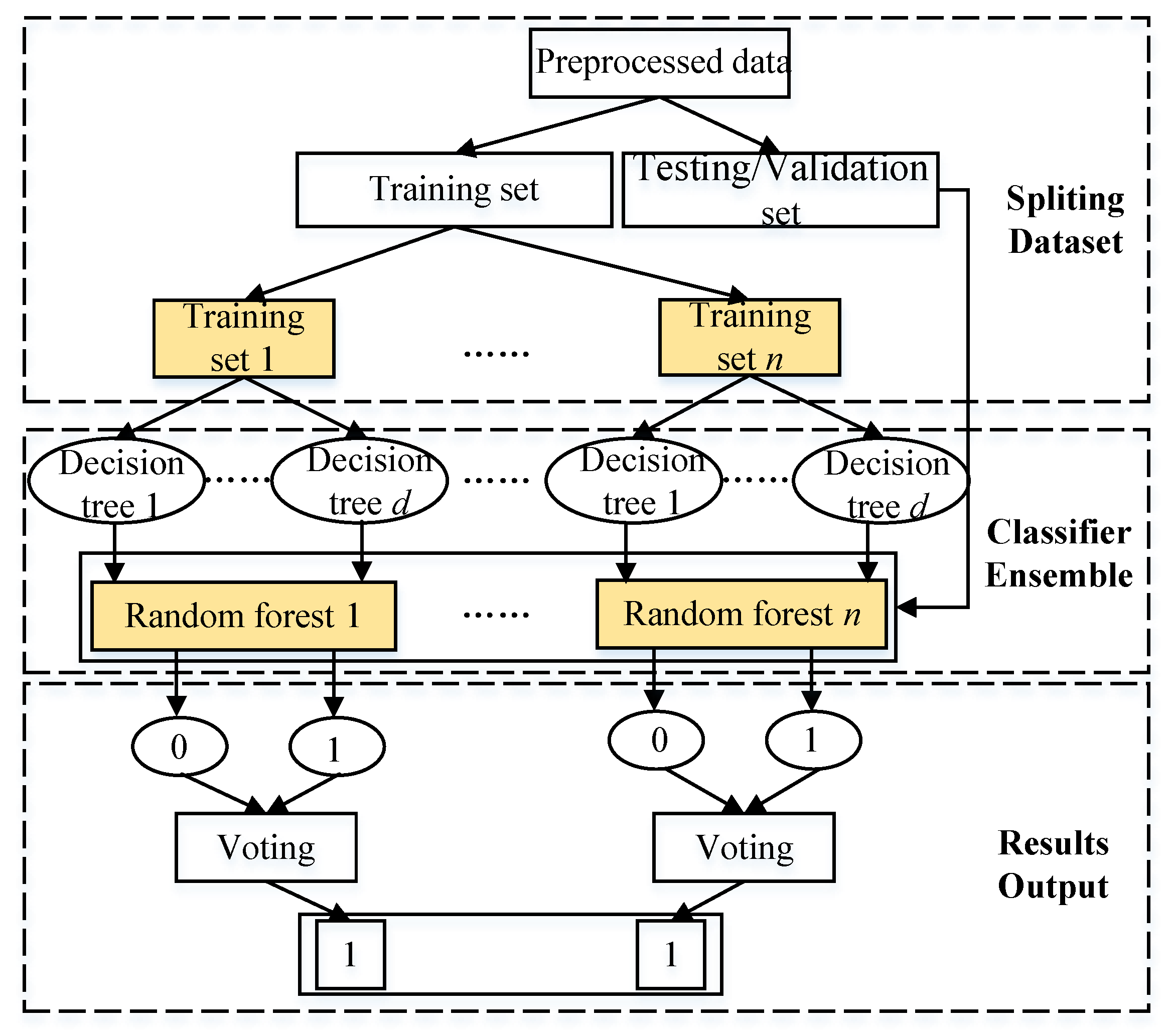
The prediction for control strategy in this study is considered as a problem of multi-label classification. However, the traditional RF can only achieve single-label classification. Therefore, the algorithm needs to be improved; correspondingly, we transform the problem into the integration of several two-class classification problems. That is, the RF is designed as a two-class classifier, and a single random forest is used to predict one of the notches of electric braking or regimes of air braking application and release. Based on these ideas, the realization of ML-RF is completely presented in Figure 3. Obviously, the integrated mechanism of random forests is used, and the idea of parallel processing is considered again.

1.

Generate sub training data set (Training set 1, …, Training set n).

For the training data set with m samples, k features, and n categories, the samples with same category are classified into one class and the rest are another class. Do this among all categories.

2.

Construct decision trees in a forest (Decision tree 1, …, Decision tree d).

• New training data set S_d is randomly sampled from the sub training set n through the replacement method; usually, the new training data sets are the same size m as that of the original sub one, and there will be a repetition between them.
• Candidates at each split node are randomly sampled from k features.
• The set S_d is used and the selected features are considered to build a tree.
• Repeat until all decision trees are constructed.
  In this paper, the determination about the number of trees and number of selected features will be discussed in Section 3.4.

3.

Construct a random forest.

The decision trees built above are used to construct a random forest.

4.

Repeat the process in steps 2–3 until n random forests are constructed.

5.

Determine the classification result according to the voting selection of the decision trees.

The schematic of decision trees that constitute a random forest is given in Figure 4.

3.3. Performance Metrics

According to the multi-label classification evaluation method proposed by Tsoumakas et al. [28], we use Hamming Loss, Accuracy Score, Jaccard Similarity, and F1 Score as evaluated by one averaging scheme: macro. Some notations introduced in [29] are used here, as shown in

Table 1. Definition of notations.

Notations	Meanings
$X$	the set of objects used for evaluation
$L$	the set of labels that spans the output space y
$\overline{x}$	an object undergoing classification
$h\left(\overline{x}\right)$	the label set assigned to object $\overline{x}$ by the evaluated classifier h
$\overline{y}$	the set of true labels for $\overline{x}$
tpj fpj fnj tnj	true positives, false positives, false negatives and true negatives of the label Lj, counted per label over the output of classifier h on the set of testing objects $\overline{x} \in$X, i.e., h(X)
$⟦p⟧$	the operator that converts logical value to a number, i.e., it yields 1 if p is true and 0 if p is false.
$\otimes$	denotes the logical exclusive or.

.

• Hamming Loss evaluates the inconsistency between predicted labels and true labels for an object.

$$Hloss\left(h\right)=\frac{1}{\left|X\right|}{\displaystyle {\sum }_{\overline{x}\in X}\frac{1}{\left|L\right|}{\displaystyle {\sum }_{L_j\in L}⟦L_j\in h\left(\overline{x}\right)\otimes \left(L_j\in \overline{y}\right)⟧}}$$

(11)

• Accuracy Score evaluates the objects whose predicted labels are exactly the same as the true labels.

$$Accuracy\left(h\right)=\frac{1}{\left|X\right|}{\displaystyle {\sum }_{\overline{x}\in X}⟦h\left(\overline{x}\right)=\overline{y}⟧}$$

(12)

• Jaccard Similarity is a method of similarity measure, and evaluates the coefficient of the size of the intersection and the union between the predicted labels and true labels.

$$Jaccard\left(h\right)=\frac{1}{\left|X\right|}{\displaystyle {\sum }_{\overline{x}\in X}\frac{h\left(\overline{x}\right)\cap \overline{y}}{h\left(\overline{x}\right)\cup \overline{y}}}$$

(13)

• F1 Score is a comprehensive evaluation method that takes into account both the precision and recall of the model by the introduction of the harmonic means. Precision is the proportion of actual positives in all classified positives, and recall is the proportion of actual positives that are correctly classified. Macro-averaging is taken to calculate the average of them.

$$precisio{n}_{\mathrm{macro}}\left(h,j\right)=\frac{t{p}_j}{f{p}_j+t{p}_j}$$

(14)

$$recal{l}_{\mathrm{macro}}\left(h,j\right)=\frac{t{p}_j}{f{n}_j+t{p}_j}$$

(15)

$$F{1}_{\mathrm{score}}\left(h,j\right)=2\cdot \frac{precisio{n}_{\mathrm{macro}}\left(h,j\right)\cdot recal{l}_{\mathrm{macro}}\left(h,j\right)}{precisio{n}_{\mathrm{macro}}\left(h,j\right)+recal{l}_{\mathrm{macro}}\left(h,j\right)}$$

(16)

$$F{1}_{\mathrm{score}}\left(h\right)=\frac{1}{\left|L\right|}{\displaystyle \sum _{j=1}^{\left|L\right|}F{1}_{\mathrm{score}}}\left(h,j\right)$$

(17)

Among the evaluation metrics, except for Hamming Loss, the larger the values of others are, the better the performance of the model is.

3.4. Parameters Determination

In this study, three parameters are primarily considered. Among these, n_tree is the number of trees in the forest; n_fea is the number of features considered in constructing the decision tree, and m_dep is the maximum depth of each tree in the forest. The optimal values of each are determined by the following algorithm, and the remaining parameters are left to the default values.

To obtain the optimal parameters for ML-RF, the 10-fold cross-validation is adopted. Taking n_tree, for example, the generalization model performance under different values was evaluated with the metrics just described. The process is shown in Algorithm 1.

Algorithm 1: The algorithm of parameter determination

Input: data set T, the range of ntree: [nmin, nmax]

Output: the optimal ntree

1: The data set T is randomly divided into 10 groups to get the data subset T1, T2, …, T10, and then one of these groups is selected as the validation data set, and others are the training data set;

2: Select ntree = nv, nv ∈ [nmin, nmax], and calculate the four evaluation metrics when one of 10 data subsets is used as a validation set in turn, then apply the averaging process to the evaluation metrics obtained;

3: Select different values for nv, repeat step 2, and save the calculation results;

4: Find the optimal value of each evaluation metric, save the corresponding value of nv, and statistic occurrence frequency of each value;

5: Output the value with the highest frequency, that is, the optimal ntree.

4. Simulation Results

4.1. Data Set

The experimental data sets are selected from the long and steep downgrades of a heavy-haul railway in China, the train traction weight is about 10,000 t, the maximum value of slope is 12‰, and the neutral zones are located on the slopes with values greater than 8.3‰, with a total of 11,450 samples. During the heavy haul train operation, the speed is controlled jointly by the electric braking and air braking.

4.2. Results Analysis

4.2.1. Optimal Parameters

The algorithm designed in Section 3 is adopted, and Figure 5, Figure 6 and Figure 7 show the evaluation results of ML-RF with different n_tree, different n_fea, and different m_dep, respectively. It is clear that when n_tree is 45, the maximum Accuracy Score, the maximum Jaccard Similarity, the maximum F1 Score, and the minimum Hamming Loss are obtained, with the same trend when n_fea is 4 and m_dep is 6. Those indicate that the best performance of ML-RF has been achieved.

4.2.2. Performance for Test Data Set

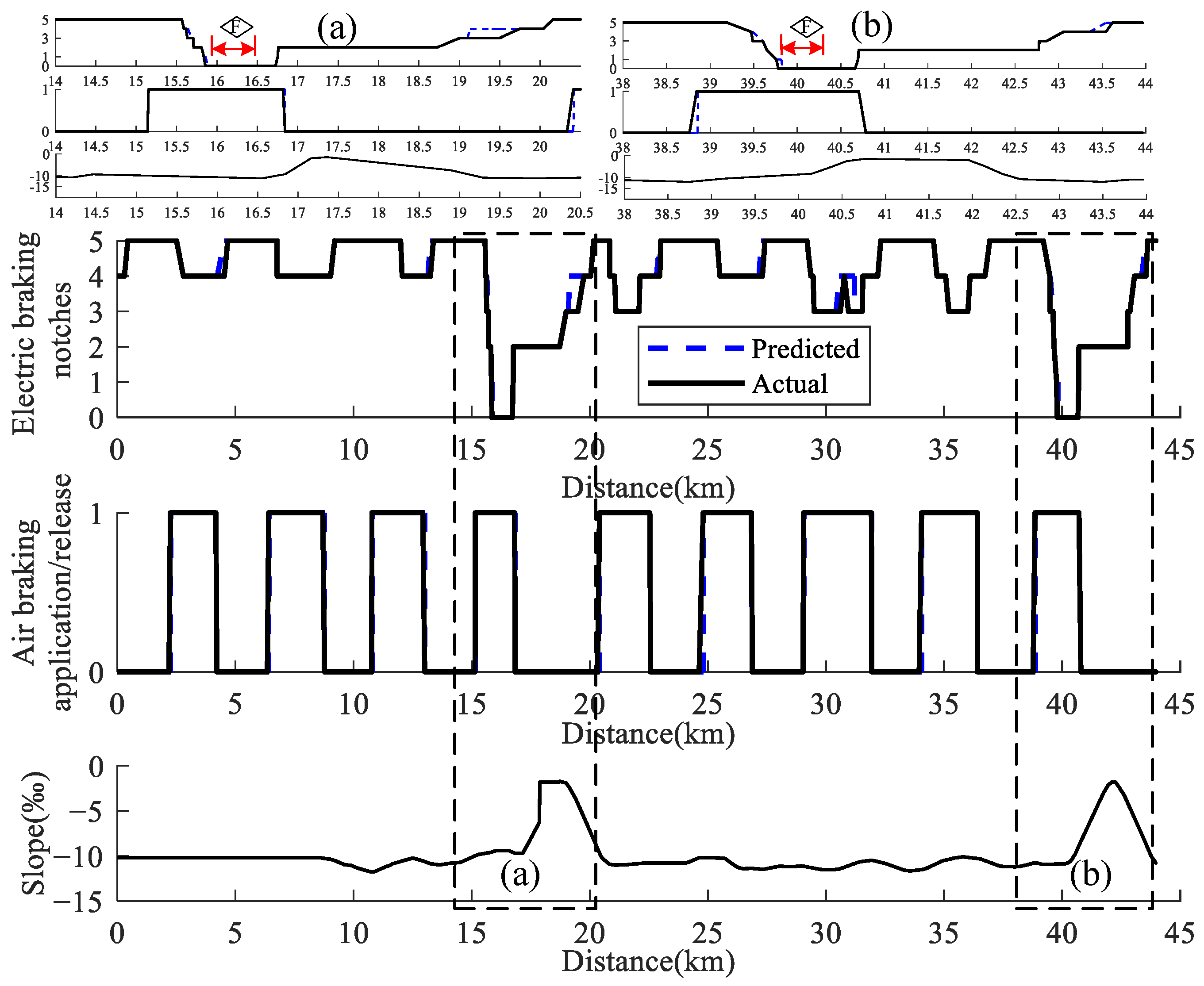
Based on the optimal ML-RF model, two sections of long and steep downgrades with a length of 29 km and 44 km, called scenario 1 and scenario 2, are chosen for the model testing. In scenario 1, there is one neutral zone, located in an area of 22.46 km to 22.98 km. In scenario 2, two neutral zones are included, located in an area of 15.90 km to 16.42 km, and 39.76 km to 40.29 km. The testing results are as follows.

Three famous algorithms, multi-label Adaboost (ML-Adaboost), multi-label support vector machine (ML-SVM), and multi-label knearest neighbor (ML-KNN), are used for comparison.

Table 2. Scenario 1: comparison with other methods.

Method	Accuracy Score	Jaccard Similarity	F1 Score	Hamming Loss
ML-RF	0.8661	0.9100	0.9330	0.0325
ML-Adaboost	0.7991	0.8735	0.9218	0.0434
ML-SVM	0.7723	0.8504	0.8142	0.0466
ML-KNN	0.5938	0.6786	0.6556	0.0982

and

Table 3. Scenario 2: comparison with other methods.

Method	Accuracy Score	Jaccard Similarity	F1 Score	Hamming Loss
ML-RF	0.9370	0.9563	0.9125	0.0147
ML-Adaboost	0.8483	0.9120	0.9003	0.0274
ML-SVM	0.8946	0.9235	0.8021	0.0222
ML-KNN	0.7095	0.7931	0.6605	0.0652

show the performance of the four algorithms. The results show that the multi-label classification algorithm based on RF, i.e., ML-RF, has the best performance on control strategy prediction.

Furthermore, the comparison of control strategies between prediction and actual operation of two scenarios are shown in Figure 8 and Figure 9. For air braking and electric braking control, the blue dotted line represents the predicted, and the black solid line represents the actual. Accordingly, the train operation curves under the predicted control strategies are shown in Figure 10 and Figure 11.

After testing, the results show that:

• From the perspective of evaluation metrics, the average values of Accuracy Score, Jaccard Similarity, F1 Score, and Hamming Loss reach up to 0.9016, 0.9332, 0.9228, and 0.0236, respectively. All of those show that the error rate of the prediction model for two kinds of braking is low, and the consistency of the predicted value and actual value is high.
• From the perspective of ensuring train operation safety, it can be seen from Figure 8 and Figure 9 that, for the HHTs running on long and steep downgrades, under the line conditions shown in the simulation, the reasonable electric braking force is used in the air braking release stage, which provides a guarantee for air-filled time. Figure 10 and Figure 11 show the HHT runs within the speed limit.
• When the train runs in the neutral zone, the electric braking force is zero. Before entering, the train is always in the release regime to prepare for the braking, because there are long and steep downgrades in this section. Through the discussion, it can be seen that the coordination of air braking and electric braking control is good.
• From the analysis of adaptability to different train operation status, although the slope of the line from 6.5 km to 29 km in scenario 1 is the same as the line from 0 km to 22.5 km in scenario 2, the control strategies for air braking and electric braking are different due to the different initial running speed of the train.

All mentioned above indicate that the proposed method in this paper is feasible.

5. Conclusions

This paper studies the control strategy of HHTs on long and steep downgrades. A learning method called ML-RF is proposed, providing a potential solution for the coordination of electric braking and air braking control on long and steep downgrades. The optimal parameters of the model are configured by combining actual running data and performance metrics. In comparison with other popular methods such as ML-Adaboost, ML-SVM and ML-KNN, the proposed model has shown a better performance on the real railway data. The average values of Average Score, Jaccard Similarity, F1 Score, and Hamming Loss are 0.9016, 0.9332, 0.9228, and 0.0236, respectively. These demonstrate that the ML-RF can be effectively applied to the prediction of HHT control strategy.

In future work, we plan to study this problem in combination with the actual notches of electric braking force and extend the strategy to automatic train operation.

References

1. Shi, J.; Ren, S.J.; Zhang, M.R. Model-based assessment of longitudinal dynamic performance and energy consumption of heavy haul train on long-steep downgrades. Transport 2019, 34, 250–259. [Google Scholar] [CrossRef] [Green Version]
2. Zhou, H.X.; Sheng, W.P.; Liu, H.E. A Modeling Method for the Driving Process of Heavy-Haul Train Based on Multi-Mass Model. IEEE Access 2020, 8, 185548–185556. [Google Scholar] [CrossRef]
3. Mcclanachan, M.; Cole, C. Current train control optimization methods with a view for application in heavy haul railways. Proc. Inst. Mech. Eng. F J. Rail Rapid Transit 2012, 226, 36–47. [Google Scholar] [CrossRef]
4. Yang, Y.Q.; Mao, B.H.; Wang, M. Research on freight train operation control simulation on long steep down lines. ASCE-ASME J. Risk Uncertain. Eng. Syst. Part A Civ. Eng. 2021, 7, 05021003. [Google Scholar] [CrossRef]
5. Yang, X.G.; Wei, W. Comparative Study on Simulation and Experiment of Heavy Haul Train Operating Conditions. J. Transp. Technol. 2019, 8, 129–137. [Google Scholar]
6. Yang, M.; Wang, K.Y.; Shi, Z.Y.; Ge, X.; Zhou, Y.C. Release performance of heavy-haul train based on electric-pneumatic blend braking. J. Chongqing Univ. Techno. (Nat. Sci). 2017, 31, 84–89. [Google Scholar]
7. Sun, Z.Y.; Wang, C.M. Security problems of operation heavy haul trains on the long heavy down grade. Railw. Locomot. Car 2009, 29, 4–7. [Google Scholar]
8. Du, K.B.; Zhang, Z.F.; Wen, Y.L. Research on autonomous driving control technology for heavy haul train. Control. Theory Appl. 2020, 31–35. [Google Scholar] [CrossRef]
9. Spiryagin, M.; Wolfs, P.; Cole, C.; Spiryagin, V.; Sun, Y.Q.; McSweeney, T. Design and Simulation of Heavy Haul Locomotives and Trains; CRC Press: Boca Raton, FL, USA, 2016. [Google Scholar]
10. Cole, C. Longitudinal train dynamics. In Handbook of Railway Vehicle Dynamics; Chapter 9; Taylor & Francis: London, UK, 2006; pp. 239–278. [Google Scholar]
11. He, F.H.; Zhang, B. Study on Brake control strategies for 20 kt combined heavy haul train under special working condition. In Proceedings of the 9th International Heavy Haul Conference on Heavy Haul and Innovation Development, Shanghai, China, 22–25 June 2009; pp. 617–623. [Google Scholar]
12. Dong, K.Y.; Wei, W. Optimizing of cycle braking of 10,000 t train on long heavy down grade of Shenshuo. J. Dalian Jiaotong Univ. 2017, 38, 17–20. [Google Scholar]
13. Zhang, X.F.; Lin, H.Q.; Zheng, M.H.; Lu, X.H. Study on air brake application and energy-saving strategy for 30 t axle load in long heavy down grade of Shenchi-Huanghua Railway. J. China Railw. Soc. 2018, 40, 63–69. [Google Scholar]
14. Yang, H.; Ma, H.P.; Fu, Y.T.; Li, Z.Q. Brake strategy for heavy-haul train based on multi-particle model. J. Beijing Univ. Technol. 2020, 46, 169–179. [Google Scholar]
15. Lin, X.; Wang, Q.Y.; Wang, P.L.; Sun, P.F.; Feng, X.Y. The energy-efficient operation problem of a freight train considering long-distance steep downhill sections. Energies 2017, 10, 794. [Google Scholar] [CrossRef]
16. Yu, H.Z.; Huang, Y.N.; Wang, M.Z. Research on operating strategy based on particle swarm optimization for heavy haul train on long down-slope. In Proceedings of the 2018 21st International Conference on Intelligent Transportation Systems (ITSC), Maui, HI, USA, 4–7 November 2018; pp. 2735–2740. [Google Scholar]
17. Huang, Y.C.; Su, S.; Liu, W.T. Optimization on the driving curve of heavy haul trains based on artificial bee colony algorithm. In Proceedings of the 2020 23rd International Conference on Intelligent Transportation Systems (ITSC), ELECTR NETWORK, Rhodes, Greece, 20–23 September 2020; pp. 1–6. [Google Scholar]
18. Su, S.; Huang, Y.; Liu, W.T.; Tang, T.; Cao, Y.; Liu, H.J. Optimization of the speed curve for heavy-haul trains considering cyclic air braking: An MILP approach. Eng. Optim. 2022, 1–15. [Google Scholar] [CrossRef]
19. Wang, X.; Tang, T.; He, H. Optimal control of heavy haul train based on approximate dynamic programming. Adv. Mech. Eng. 2017, 9, 1687814017698110. [Google Scholar] [CrossRef] [Green Version]
20. Wang, X.; Li, S.K.; Tang, T.; Xun, J. Intelligent operation of heavy haul train with data imbalance: A machine learning method. Knowl-Based Syst. 2019, 163, 36–50. [Google Scholar] [CrossRef]
21. Huang, Y.N.; Tan, L.T.; Chen, L.; Tang, T. A neutral network driving curve generation method for the heavy-haul train. Adv. Mech. Eng. 2016, 8, 1–14. [Google Scholar] [CrossRef] [Green Version]
22. Wei, S.Y.; Zhu, L.; Chen, L.J.; Lin, Q.Q. An adaboost-based intelligent driving algorithm for heavy-haul trains. Actuators 2021, 10, 188. [Google Scholar] [CrossRef]
23. Tang, H.Y.; Wang, Y.; Liu, X.; Feng, X.Y. Reinforcement learning approach for optimal control of multiple electric locomotives in a heavy-haul freight train: A Double-Switch-Q-network architecture. Knowl-Based Syst. 2020, 190, 105173. [Google Scholar] [CrossRef]
24. Bai, Y.; Mao, B.H.; Ho, T.; Feng, Y.; Chen, S.K. Station Stopping of Freight Trains with Pneumatic Braking. Math. Probl. Eng. 2014, 2014, 1–7. [Google Scholar] [CrossRef]
25. Zhang, M.L.; Zhou, Z.H. A review on Multi-label Learning Algorithms. IEEE Trans. Knowl. Data Eng. 2014, 26, 1819–1837. [Google Scholar] [CrossRef]
26. Wu, Q.H.; Wang, H.H.; Yan, X.S.; Liu, X.B. MapReduce-based adaptive random forest algorithm for multi-label classification. Neural Comput. Appl. 2019, 31, 8239–8252. [Google Scholar] [CrossRef]
27. Wang, Z.Y.; Wang, Y.R.; Zeng, R.C.; Srinivasan, R.S.; Ahrentzen, S. Random Forest based hourly building energy prediction. Energy Build. 2018, 171, 11–25. [Google Scholar] [CrossRef]
28. Tsoumakas, G.; Katakis, I.; Vlahavas, I. Mining multi-label data. In Data Mining and Knowledge Discovery Handbook; Springer: Berlin/Heidelberg, Germany, 2009; pp. 667–685. [Google Scholar]
29. Szymański, P.; Kajdanowicz, T.; Kersting, K. How is a data-driven approach better than random choice in label space division for multi-label classification? Entropy 2016, 18, 282. [Google Scholar] [CrossRef] [Green Version]
Figure 1. Long and steep downgrades.
Actuators 11 00145 g001
Figure 2. Prediction of control strategy.
Actuators 11 00145 g002
Figure 3. Implementation of ML-RF.
Actuators 11 00145 g003
Figure 4. Schematic diagram of one random forest.
Actuators 11 00145 g004
Figure 5. Evaluation results of ML-RF with different number of trees in the forest (ntree). (a) Accuracy Score; (b) Jaccard Similarity; (c) F1 Score; (d) Hamming Loss.
Actuators 11 00145 g005
Figure 6. Evaluation results of ML-RF with different number of features selected as candidates at each split (nfea). (a) Accuracy Score; (b) Jaccard Similarity; (c) F1 Score; (d) Hamming Loss.
Actuators 11 00145 g006
Figure 7. Evaluation results of ML-RF with different maximum depth of tree (mdep). (a) Accuracy Score; (b) Jaccard Similarity; (c) F1 Score; (d) Hamming Loss.
Actuators 11 00145 g007
Figure 8. Scenario 1: comparison of predicted and actual control strategy. (a) Section from 19.3 km to 25 km.
Actuators 11 00145 g008
Figure 9. Scenario 2: comparison of predicted and actual control strategy. (a) Section from 14 km to 20.5 km. (b) Section from 38 km to 44 km.
Actuators 11 00145 g009
Figure 10. Scenario 1: train operation curve under predicted control strategy.
Actuators 11 00145 g010
Figure 11. Scenario 2: train operation curve under predicted control strategy.
Actuators 11 00145 g011