1. Introduction
Condition monitoring compares a rotor system’s actual behavior with a desired or normal behavior using indicators to detect faults. In [
1], multiple rotor faults are described using minimal models. Displacement and force orbits are used as indicator functions that are used in combination with models for different rotor faults. Indicator functions can be, for example, frequency response functions (FRFs) or modal parameters. Mechanical FRFs
are defined as the linear relationship between harmonic forces
and harmonic responses
(displacement, velocity or acceleration), which depend on the excitation frequency
, cf. [
2]:
Obtaining the FRFs in simulation models requires low effort, as long as the model size is not too large. For a symmetric rotor, considering gyroscopic effects, the FRFs for a rotational speed
can be obtained by, cf. [
3]:
with the system’s mass, damping, gyroscopic and stiffness matrix represented as
and respectively.
To estimate the FRF from a set of given input (force) to output (response) time-signals, a number of algorithms, based on fast Fourier transforms, exist. Experimentally determining the FRFs of rotating systems is a special challenge. The FRFs obtained from measurement are often used in experimental modal analysis (EMA) to determine the modal properties of the system.
In order to measure the FRFs of a system, typically, its operation must be stopped. The system must be instrumented by exciters and sensors. Stopping the system’s operation and performing the tests takes a lot of time and effort. So, this is not feasible for condition monitoring.
In this contribution, the AMBs are used as combined exciters and sensors while still being used as bearings. This enables us to measure the FRFs of the rotor system during operation and thus avoids the need to stop its operation.
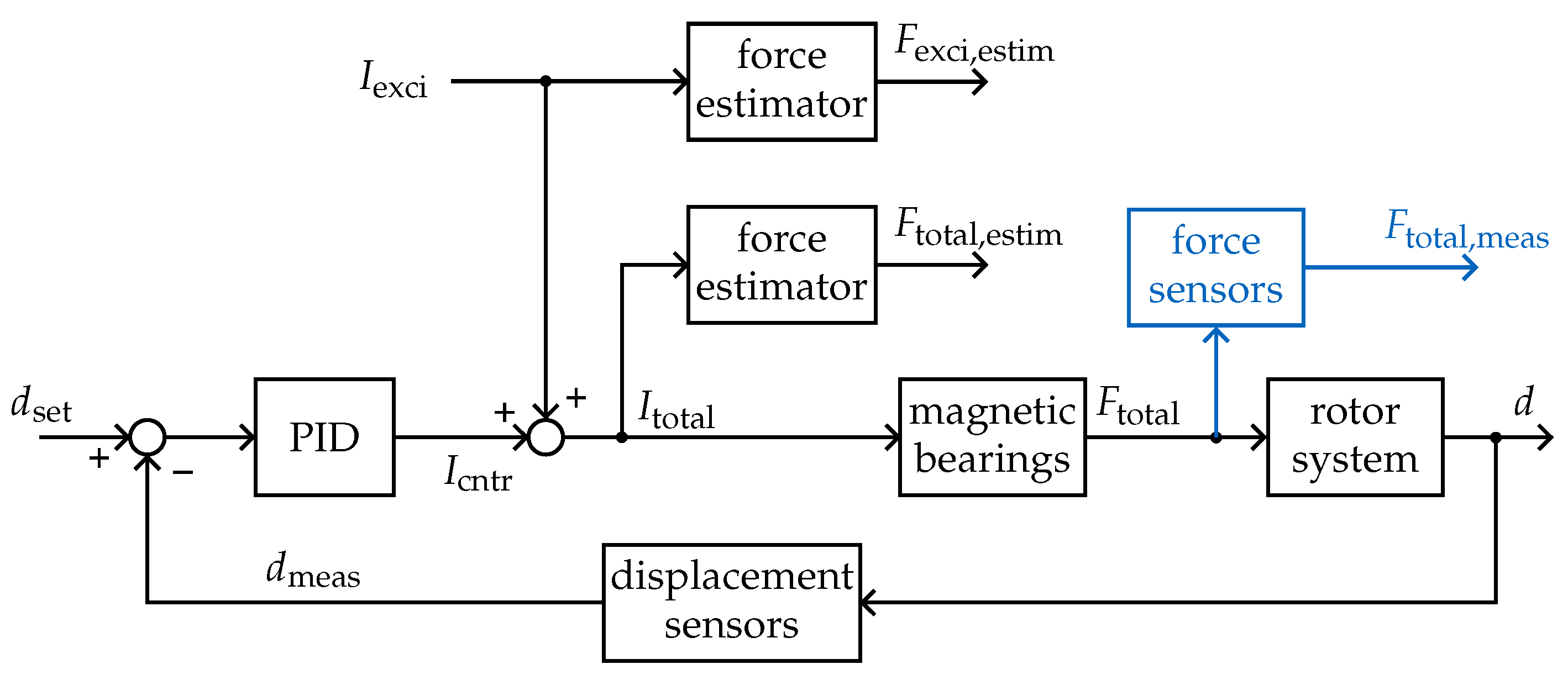
The force in the active magnetic bearings for normal operation is set by a current from its PID-controller. To measure the system’s FRFs, an additional excitation current is added to the controller current. This is called the excitation force. The total force includes both the controller and the additional excitation force.
The excitation force and the total force in the bearing is estimated by a linear current–force relationship. With this, it is possible to determine the FRFs of the supported system and of the free rotor in a single measurement run. Thus, FRFs can be used for a continuous condition monitoring of the rotor system. Knowing both the free and the supported FRFs of the rotor is especially useful for localizing faults in the rotor system, as the bearing effects can be separated from the rotor effects in the different FRFs.
Many publications have treated the identification of bearing parameters. In the review paper [
4], a comprehensive summary of identification techniques using vibration signals is given. Different excitation sources can be used to obtain the necessary vibration signals. For example, Refs. [
5,
6,
7] use the excitation from a mass unbalance to determine the bearing parameters. Impact excitation is commonly used in structural dynamics identification but can also be used for rotating systems. In [
8], an impact excitation is applied through an intermediate ball bearing on a rotating disc. In [
9], impact testing is applied to a non-rotating rotor in magnetic bearings to obtain FRFs, which are used to improve the AMBs’ control. A natural idea in rotor systems with AMBs is to use them for an excitation of the system. An overview of the state-of-the-art AMBs can be found in [
10], where there is a section dedicated to condition monitoring using AMBs.
An overview of strategies to measure FRFs of rotating systems have been proposed in the BRITE/MARS project [
11], also discussed in [
3]. In these publications, active magnetic bearings (AMBs) are used as an excitation system in addition to the existing support in ball bearings. Similarly, in [
12], a bearingless motor is used to excite a system with oil-film bearings. Related work can also be found in [
13], where the parameters of the oil-film bearings and the bearingless motor are identified through a regression by varying unbalance and controller parameters. In [
14], an excitation device similar to magnetic bearings is used to identify the dynamics of a machine tool spindle assembly. In [
15], an approach for combining the AMB’s control system with a MIMO identification procedure to obtain a state-space model is given for systems with real poles. In [
16,
17], a method to combine the magnetic bearing’s support with an additional excitation is given. This is similar to the method applied in this contribution. In [
18], an approach of using AMBs to perform EMA of the supported rotor system using an external commercial modal analysis system was shown for the levitating but non-rotating rotor. Furthermore, [
16] discusses the possibility to measure the FRF of the free rotor in AMBs but unfortunately does not give results. In the aforementioned publications, except for [
16], the FRF of the free rotor could not be measured.
In this contribution, the FRFs of the free and supported rotor can be measured simultaneously with one setup that is suitable for practical applications, see also
Section 2.4. The excitation is applied via the bearings, using an additional excitation current that is added to the AMBs’ controller currents. The combination of the excitation and bearing task in the magnetic bearing enables us to measure the FRFs of different theoretical system configurations in a single experiment by considering different force signals, which has not been shown in the literature. The basic idea can be summarized as follows: Considering only the excitation force, which is a perturbation added to the controlled bearing force, the FRF of the supported rotor is obtained. Considering the total force, namely, the sum of contributions from the controller and from the additional excitation, gives the FRF of the free rotor. Here, we want to use a simple implementation of a standard MIMO excitation signal, e.g., burst random excitation, which can be found in text books about EMA, for example, in [
2] (p. 323ff). We also want to give an intuitive interpretation of the results to understand how AMBs can be used to obtain different FRFs of one system in a single experiment.
The approach is applied to an academic test rig with and without rotation. First, the methodology is presented in
Section 2 with the academic test rig as an example. The academic test rig, the experimental procedure, and the simulation model are outlined, and requirements for applying the methodology to a practical application are discussed. Results obtained with the proposed approach for a non-rotating system are given and interpreted in
Section 3. The method is then also applied to a rotating system in
Section 4. A short outlook on how to estimate the bearing dynamics from the obtained FRFs is given in
Section 5. In the end, a short summary and conclusions of the contribution are given.
3. Non-Rotating System
The experimental results for the non-rotating system are obtained in a single measurement and are validated by comparison with simulation results.
3.1. FRF of the Rotor in AMBs Using Additional Excitation Force
In a first step, only the additional excitation force on the AMBs is considered as an input to the FRF calculation algorithm. The excitation force is estimated from the linear static relationship in Equation (
5).
Figure 5 shows a simplified model of the resulting system. As only the additional excitation force is considered, the bearings forces are considered as internal forces and thus are included in the dynamic FRF. The abbreviation
supp is used for the
supported system.
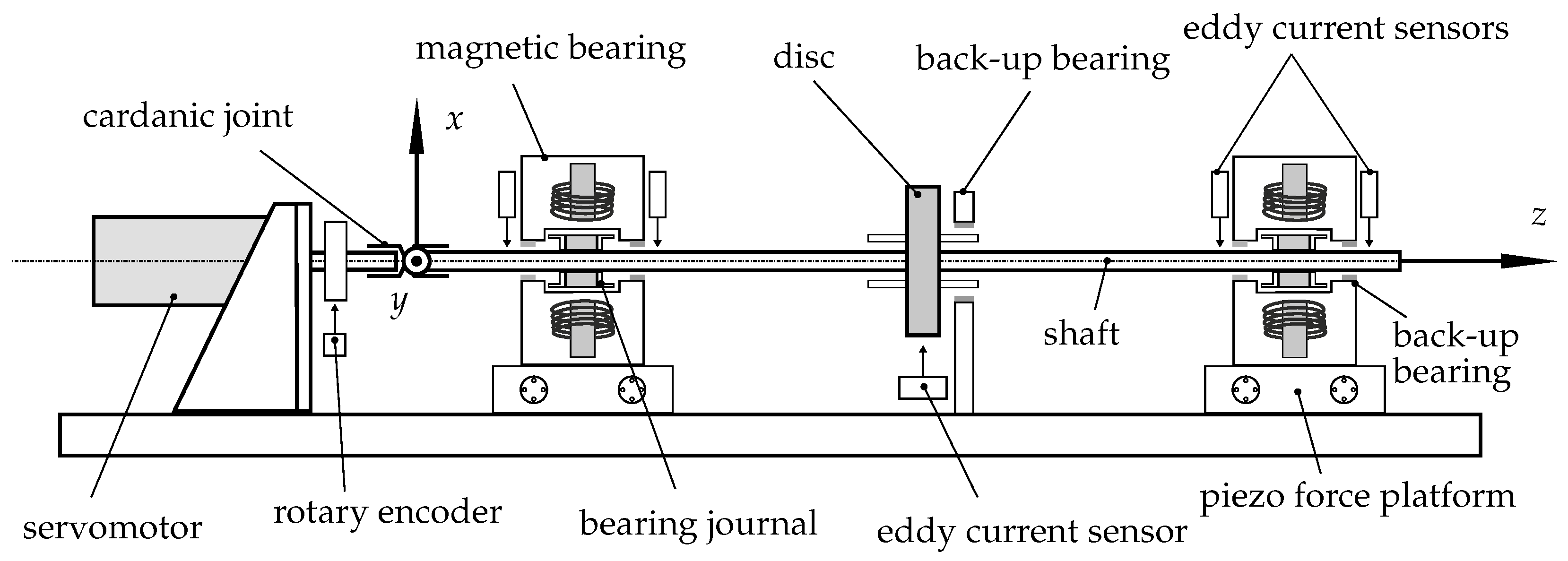
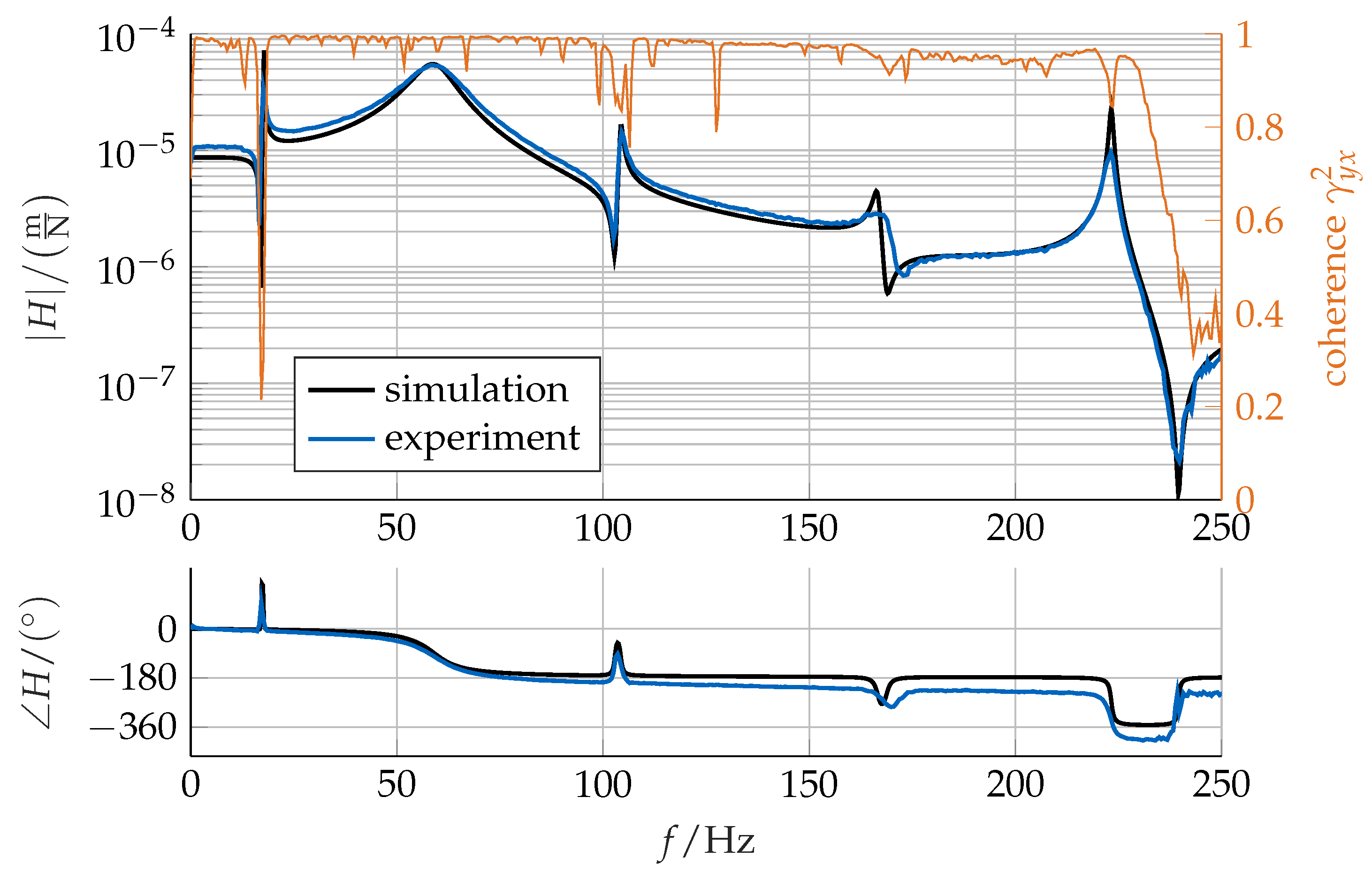
Figure 6 shows the experimental results for the FRF using only the additional excitation force and compares them with the results from the numerical simulation for the rotor in elastic bearings. It shows the FRF between excitation at the right AMB and the response at the rightmost eddy current sensor. The excitation and response positions are very close, so a behavior similar to a driving point FRF is expected. The experimental and simulation results are clearly similar. The coherence of the experimental FRF is shown in orange. It starts to fall at around 200 Hz because a band-limited noise with a cut-off frequency of 250 Hz was used in the burst random excitation.
The frequency of the peaks in simulation and experiment agree very well. There is a slight difference for the peak at around 165 Hz. The damping of the modes can be qualitatively seen from the sharpness of the peaks. For frequencies above 150 Hz, the simulation’s damping is lower than in the experiment. The peak at around 58 Hz is due to the support from the magnetic bearings. The simulation model agrees well for this peak thanks to the model updating procedure, described in
Section 2.3. The depicted FRF does not completely show a driving point behavior, which can be seen by the missing anti-resonance between the resonance-peaks at 105 and 168 Hz. This can be observed in both experiments and simulations and is due to the distance between the excitation and response points.
There is an offset in the amplitude between the experimental and simulation results. This is due to imperfections in determining the current–force factor .
The phase of the FRF shows a similar behavior in simulation and experiment. As expected, the phase falls by 180° for resonances and rises by 180° at anti-resonances. The phase of the experimental FRF exhibits, however, a linear drift with frequency. This is due to effects in the current amplifier, mainly time-delay. These effects are not compensated in the static force estimation using
, see Equation (
4).
Both curves show anti-resonances close to the resonance frequencies. This means, that the points for excitation or response measurement are very close to vibration nodes. This is due to the fact that the considered excitation and response locations for the measurements are directly at the AMB. The AMB’s controller tries to minimize the displacement because it acts as a bearing. Naturally, the vibration nodes will be close to the bearing. The close vicinity of the excitation and measurement points to the bearing is a disadvantage of the method and can be interpreted as a bad observability and controllability at these points. The stiffer the AMBs are tuned, the worse the problem becomes.
This also means that the resulting FRFs are very sensitive to the exact positioning of the sensors as they are close to the vibration nodes. Small mistakes in the position have a rather large influence on the measured FRFs. So, an inherent problem of the method is that the excitation position is very close to the vibration nodes.
This experiment showed the measurement of the supported rotor FRF with a force estimation using only the additional excitation current.
3.2. FRF of the Free Rotor Using Total Force
In this section, the total force of the AMB is considered for the FRF calculation algorithm.
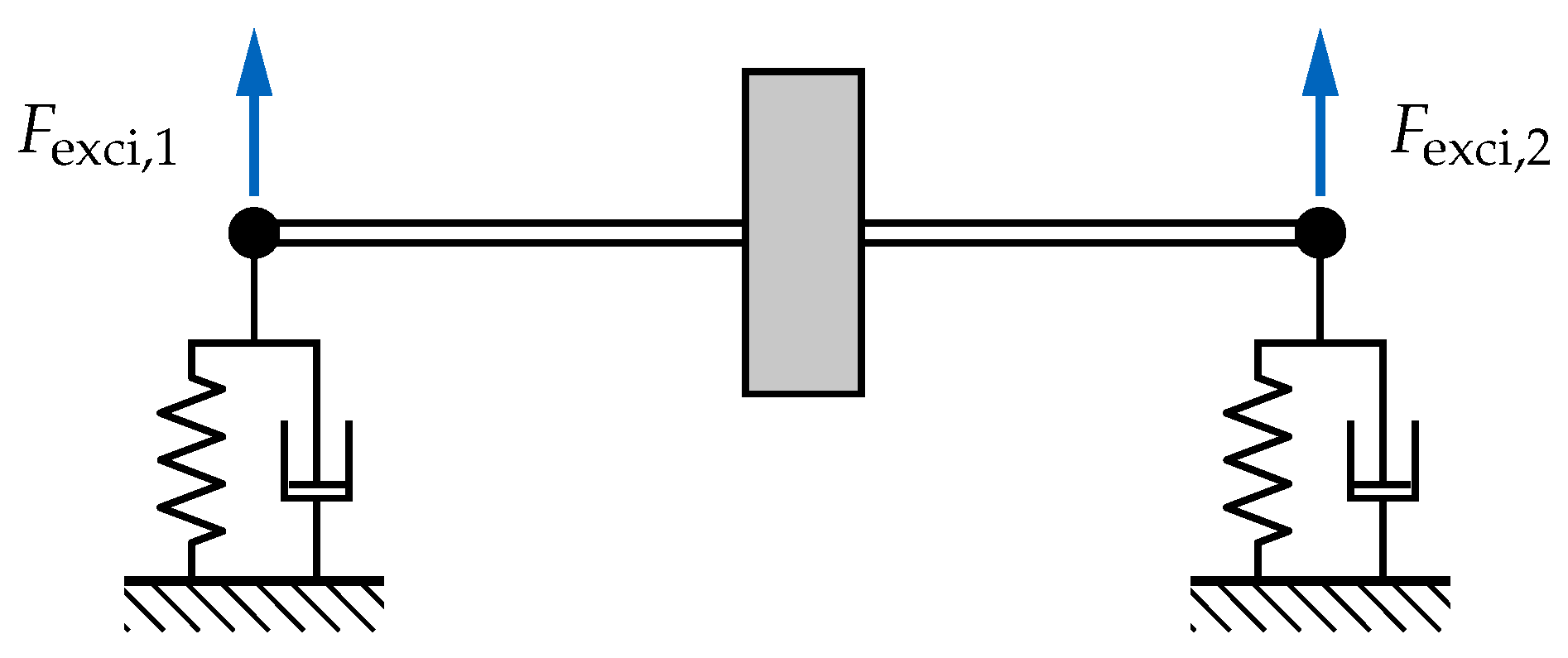
Figure 7 shows the rotor that is cut free from the bearings.
The total force is estimated from Equation (
5) and measured by the force platforms. It is the force that acts between the ground and the magnetic bearings. It includes the additional excitation force and the controller force. The controller force can be seen as the reaction force of the bearings. It is now assumed to be part of the external excitation and the bearings are therefore no longer part of the characterized system. So, only the rotor without the bearings remains, i.e., the free rotor:
For this example, the estimated total force is used and compared with the results from the measured total force. There are several methods to determine the total force. In [
16], some possibilities are given. We summarize them in the order of increasing abstraction, i.e., starting from a method using a simple model to methods using more advanced models:
Measuring the force between the AMB and the ground. This is applied here using the piezo force platforms as validation for the results involving a more complicated model. It is suggested to consider the inertia of the AMB. For this work, the inertia is not considered because the force platform is assumed to be rigid and rigidly fixed to the testbed.
Measuring the magnetic flux density B using a Hall-sensor in the AMB and estimating the force using the area of the electromagnet and the magnetic permeability constant. This method enables the magnetic bearing to measure the total force, without using additional force sensors, making the AMB a self-sensing active component. It requires a simple model for the relationship between flux density B and the force F.
Estimating the force from a more comprehensive model using the electrical current. This can be a model which has been parameterized experimentally or which used theoretical knowledge about the AMBs from an electromagnetic simulation model.
One way is to directly measure the current. Current measurement is much cheaper and more easily available than, for example, force measurement.
Another way is to estimate the current from the controller’s output. The electrical current is not measured, but guessed from the control system’s desired values. This is the method used in this work. It is assumed that the behavior of the electrical system is ideal, i.e., a desired current is perfectly executed. Here, the force is estimated using a linear static current–force relationship, given in Equation (
5).
Figure 8 shows the results for the experimental FRF using the total force between the right magnetic bearing and the rightmost eddy current sensor. It shows the amplitude and phase of
and its coherence for the experimental results. This experimental FRF is obtained by using signals from the same experiment that was also described previously in
Section 3.1. The curves
exp. measured total force use the force that is directly measured by the force platforms
. The curves
exp. estimated force use the force that is estimated from the total electric current
. It is compared to the simulation results for the free rotor system.
For the receptance FRF of a free system, one expects to see the effect of the rigid body modes, i.e., the amplitude starts at infinity, . This can be clearly seen in the simulation results. In the experimental results, this is less obvious. For lower frequencies, the amplitude does not match. In order for the FRF to go to infinity, the FFT of the force must go to zero, as the displacement response is bounded by the bearings. A force FFT of zero is not possible in practice, as the force signal is then primarily dominated by noise. The same effect also applies to the resonance peaks with very high FRF amplitudes. The amplitude above 6 Hz and outside of the resonance points agrees very well using the force platforms, at least up to 210 Hz.
The FRF from the estimated force approaches the correct amplitudes only after approx. 90 Hz. The FRF with the estimated force is lower than for the measured force. This implies that the force is overestimated by the force estimation. The reason for the deviation in the amplitudes is not fully clear. It is suspected that the deviation is due to not considering the effect of the displacement on the magnetic force. Due to the bias current in the coils, the magnetic bearings have a destabilizing effect, i.e., they exhibit a negative stiffness that gives a force on the journal pulling it out of the center. The P-part of the PID-controller gives a positive stiffness that acts against the displacement. The controller force acts on the journal pointing towards the center, while the negative stiffness due to the bias current creates a force pointing away from the center. This can effectively decrease the bearing force. The effect of bias current on the out-of-center journal is not considered in the linear current–force estimation, thus creating an overestimation of the force.
As in the previous section, the simulation model agrees very well with the experimental result for the measured total force. For frequencies above 150 Hz, the simulation’s damping is too low. This is caused by an imperfect model updating for the simulation model in
Section 2.3.
The free rotor has vibration nodes close to the measurement positions, which makes the system sensitive to small positioning errors. In contrast to the previous section, this is not an inherent problem of the method, but rather the case for this special rotor system, which has concentrated mass at the bearing journal while the rest of the rotor is rather slim.
Compared to the previous
Section 3.1, there is no eigenfrequency at around 58 Hz, which was found from the identification of the rotor with supports because the FRF of the free rotor is determined here, using the total force.
The phase of the FRFs show a similar behavior between simulation and experiment.
The coherence has small dips at resonance points. This is especially relevant for the first peak. The same reason, which is given above, applies: the force is very low for high FRF amplitudes, so noise has a larger effect. In
Figure 9, the ordinary coherence (correlation) between the input signals is shown. The controller force is dominant when there is large displacement that has to be controlled. At resonance frequencies of the supported system, the displacement is large and thus strongly influences the total force and thus its correlation. A high correlation of the input signals can cause problems in the FRF calculation due to the poor conditioning of the problem, cf. [
2] (p. 327).
Another effect that can negatively influence the results is internal feedback in the measured system. This can lead to biased FRFs, cf. [
3]. In magnetic bearings, the displacement/position within the magnetic bearing directly influences the magnetic force. This influence was neglected in this contribution. For a significant feedback, disturbances in the output (displacement) have an effect on the input (force), which cannot be averaged out by the used
-estimator.
3.3. Interim Conclusions
It has been shown that it is possible to measure the FRF of the supported rotor system and of the free rotor in a single measurement run. The supported system’s FRFs were experimentally determined by estimating the excitation force from the current, and the results agree well. The free rotor’s FRFs were determined by considering the total force. The experimental results using the force estimation do not reflect the amplitude well for small frequencies. In the low frequency range, the estimation is insufficient. However, the overall behavior agrees well with simulation and experimental results using measured force.
The results for the FRFs using only force estimation showed differences in amplitude compared to simulation results or to measured force FRFs. In continuous condition monitoring, the FRFs (indicator function) of a rotating machine are continuously compared to previous FRFs. So, mostly differences in the FRFs are important, while the exact amplitude is of less importance, which supports the suitability of the presented FRF acquisition using estimated forces.
4. Rotating System—FRF of Free Rotor
In this section, an example of applying the measurement method to obtain the free rotor’s FRF on the rotating system is presented shortly.
As given in Equation (
2), in simulation, the FRF of a symmetric rotor at a given speed can be easily obtained from the system matrices. In contrast, experimental measurements of the FRFs for the rotating system are hard to acquire. Especially the FRF of the rotating free rotor cannot be obtained by usual EMA techniques, e.g., using impact testing.
Using the technique shown in this contribution, the rotor is excited in its magnetic bearings, and the total force is used for FRF-estimation.
Figure 10 shows the determined FRFs in simulation and from the experiment for a rotational speed of
s
−1. Two results from the experiment are shown.
The results are similar to
Figure 8, with the damping of the simulation model still being too low. Due to the rotational speed, gyroscopic effects occur, which split the eigenfrequencies. This can be seen occurring in double peaks for the tilting modes.
At the frequency of rotation and at , which are marked in the figure, the FRF with the measured force has a small dip. The disturbance at frequency is due to unbalance. The unbalance force is not measured directly. However, the force is counteracted by both bearings and is thus indirectly measured. For a conventional impact excitation of the system, the additional unbalance force is not detected. That would lead to peaks in the FRF at multiples of the rotation frequency. Here, the unbalance force is indirectly measured. So, it cannot be predicted whether the FRF has a peak or a dip. The only possible statement is that the computed FRF should not be trusted for multiples of the rotation frequency. Outside of these critical points, the FRFs of the rotating system can be determined accurately with little disturbance from the rotation.
Figure 11 gives a summary of the experimentally determined FRFs. Each sub-figure shows the results from one measurement run, for
and
, respectively. This clearly shows the difference between the supported system’s and free rotor’s FRFs, where the rigid body modes are apparent at small frequencies for the free system and the distinct peak at around 58 Hz only appears in the supported system. By comparing the left and right parts of
Figure 11, the splitting of eigenfrequencies with rotation becomes clear.
Summary of Difficulties in the Experiments
Points that require special care in the experiments were given in this section for the rotating system and in the previous section for the non-rotating system. They are summarized here for convenience.
The biggest assumption in the method is the assumption of a linear current–force law with no influence from displacement. In combination with an imperfect calibration of the current-force factor , this can lead to bias in the FRFs from estimated forces. The phase of FRFs from estimated forces show a linear drift, which was not compensated in the presented results. The correlation between input signals in the MIMO procedure must be checked to make sure that the results are valid. In the presented experiments, this was given in a large frequency region. When using results from measured forces, high FRF amplitudes cannot be accurately determined due to noise which pollutes measurements of very low forces. For FRFs with rotation, one must keep in mind that there is a pollution due to unbalance forces and higher harmonics at multiple of the rotation frequency.
5. Decoupling of Bearing Dynamics
This section gives a short outlook on a possible method to extract the bearing dynamics from FRF measurements of the supported system and free rotor. The resulting bearing dynamics could be used as indicator functions in a condition monitoring scheme.
Dynamic substructuring allows us to combine or decouple substructures, cf. [
26,
27]. Frequency-based substructuring uses frequency response functions of dynamic systems. The so-called dynamic decoupling uses dynamic stiffnesses, which are the inverse of frequency response functions
.
Figure 12 shows the decoupling procedure to obtain the bearing dynamics. The free rotor is decoupled from the supported system, which yields the bearing dynamics, without the influence of the rotor itself. In primal decoupling, this is written as:
As an example, this procedure is applied on the results for the rotating system in
Figure 10. For the supported system, the FRFs using the estimated excitation force are used. For the free rotor, the results from the estimated total force are used. Driving point FRFs in the middle of each the bearings are obtained by averaging the displacement signals from the eddy current sensors in the front and back plate of each bearing. Only the
x-direction is considered because this is the direction of the excitation force. The rotor and bearing dynamics are taken to be axisymmetric.
The dynamic stiffness matrix of the isolated AMB is the the result of the decoupling procedure, see Equation (
8). The results of the decoupling are shown in
Figure 13. The degrees of freedom are the
x-directions in magnetic bearings 1 and 2. They are given as real and imaginary parts in sub-figures a and b, respectively.
For the real-part of
in
Figure 13a, the diagonal elements are close to a constant line, while the off-diagonal elements are close to zero. For the imaginary-part of
in
Figure 13b, the diagonal elements evolve approximately linear with the frequency, while the off-diagonal elements are again close to zero.
A simple dynamic model of the bearings can be used to model the system according to the experimental results for the dynamic stiffness of the isolated AMBs:
A simple curve fitting in the real and imaginary part can be used to obtain linear stiffness and damping of the bearings
. These identified parameters could be used in condition monitoring as indicators of the bearing condition. A large change in the bearings’ stiffness and damping could indicate a fault in the bearings.
It should be noted that the identified parameters could only be used for monitoring purposes because of the uncertainties in the exact amplitude of the estimated FRFs. For condition monitoring, changes in the values are more important than exact calibrated absolute values. For a direct joint identification, high-quality FRFs would be needed with calibrated precise amplitudes.
6. Summary and Conclusions
This contribution shows that it is possible to measure the free FRF of a rotor and the supported system’s FRF in a single measurement run using AMBs with multiple input signals. Measurement of the FRF of a rotating rotor without bearing influence could not be performed using usual impact hammer FRF measurements.
With the force estimator used in this contribution, the FRF amplitude cannot be accurately determined for low frequencies. For condition monitoring, the correct amplitude is not as critical as a continuous evaluation of the results. Thus, one could possibly use FRFs using estimated forces for condition monitoring.
The availability of FRFs of the free and the supported rotor during operation can further improve condition monitoring. It can be used to locate a possible fault. A fault in a bearing would show in the FRF of the supported rotor, but not in the FRF of the free rotor. A fault in a rotating component can be localized if it can be observed in both types of FRFs. A method to estimate the current bearing stiffness and damping was presented.
Furthermore, the possibility of measuring different FRFs during a machine’s operation can be used to continuously adjust a machine model, i.e., for parameterizing a digital twin.
Free rotor FRFs can also be used to extend frequency-based substructuring, cf. [
27], to rotating systems, which can, for example, be applied in experimental characterization of rotor system components (e.g., seals, journal bearings), see also
Section 5. This requires high-quality FRFs, i.e., force measurement or an improved force-model.


