Body Calibration: Automatic Inter-Task Mapping between Multi-Legged Robots with Different Embodiments in Transfer Reinforcement Learning

Abstract

Machine learning algorithms are effective in realizing the programming of robots that behave autonomously for various tasks. For example, reinforcement learning (RL) does not require supervision or data sets; the RL agent explores solutions by itself. However, RL requires a long learning time, particularly for actual robot learning situations. Transfer learning (TL) in RL has been proposed to address this limitation. TL realizes fast adaptation and decreases the problem-solving time by utilizing the knowledge of the policy, value function, and Q-function from RL. Taylor proposed TL using inter-task mapping that defines the correspondence between the state and action between the source and target domains. Inter-task mapping is defined based on human intuition and experience; therefore, the effect of TL may not be obtained. The difference in robot shapes for TL is similar to the cognition in the modification of human body composition, and automatic inter-task mapping can be performed by referring to the body representation that is assumed to be stored in the human brain. In this paper, body calibration is proposed, which refers to the physical expression in the human brain. It realizes automatic inter-task mapping by acquiring data modeled on a body diagram that illustrates human body composition and posture. The proposed method is evaluated in a TL situation from a computer simulation of RL to actual robot control with a multi-legged robot.

1. Introduction

Owing to the declining birth rate, aging population, and declining working population in recent times, intelligent robots will be deployed in the real world in the future. In intelligent robots such as autonomous robots, it is important to realize and implement not only hand-coding rules but also machine learning theory and the corresponding architecture. Among machine learning techniques, reinforcement learning (RL) has been attracting attention as it can actively search for solutions [1,2]. An optimal solution can be found through trial and error based on rewards. However, RL needs to be lengthy or include many trials. Transfer learning (TL) in RL is proposed for solving this problem [3,4]. TL is a method of improving the efficiency of current learning by reusing the knowledge acquired in the past. In TL for RL, the agent of the target task can improve the learning speed and adaptive performance of the target task by reusing the knowledge (e.g., policy, value-function) acquired by the agent of the source task. In the agents of the source task and target task, the effects of the physical composition and behavior on the environment need to be similar. If the agents’ configurations are different (but similar) in the source task and target task, they are described by inter-task mapping.

Inter-task mapping is defined by a human operator based on experience and intuition. The importance of mapping in the TL in RL is that it can directly change the performance of the TL, even if appropriate knowledge is transferred. A method using an ontology that supports the design of inter-task mapping has been proposed [5]. In addition, a method for learning inter-task mapping using a neural network has also been proposed [6,7,8]. These studies are limited to verification by simple computer simulation and the use of robots with low-DOF control, which are not automated. Automation of inter-task mapping between robots with multiple degrees of freedom (DOF) such as multi-legged robots has not been achieved.

In order to realize TL in RL in practical use, it is important to integrate it with other research areas and domains. DQN, which combines Q-learning and deep learning, has achieved explosive performance improvement [9]. Evolutionary TL in RL, inspired by Darwin’s theory, has also been studied [10]. A four-legged walking robot that imitates and learns the movements of animals is being studied [11]. There are also studies that apply the findings of cognitive psychology to TL in RL [12]. As mentioned above, it is possible to solve new problems by fusing with technologies and theories other than TL and RL. For the automated acquisition of inter-task mapping with high DOF, it is important to consider not only the trial-and-error process but also the embodiment of the robot and the relationships between robots. Ota investigated the mechanism of the human brain as it adapts to changes in bodily function for rehabilitation [13]. Humans have an internal model of the body in the brain called a body representation, and it has been shown that active human movements with goal-oriented and achievement feedback influence the updating of the body representation in the human brain [14]. If the functions or structures of the body are changed, the body representation is also changed to represent the actual state, in the long term. Focusing on the transformation of the human body representation, the aim of this research is to realize automatic inter-task mapping by acquiring the physicality of the robot as a diagram and describing it as a difference or transformation. In this study, RL robots are used to construct a body diagram. The environmental effects of their actions are measured using sensors mounted on the robots, and the geometric connections of each joint or motor of the robots are estimated. Furthermore, for performing TL between robots with different physicalities, a method of automatically generating inter-task mapping by computing the similarity of body diagrams is proposed.

The remainder of the paper is organized as follows. Section 2 discusses the basic theories, related work, and the approach in this paper. Section 3 presents the proposed method of automatic inter-task mapping based on a body diagram. Section 4 presents the evaluation experiment using computer simulation and actual robots such as multi-legged robots. Finally, Section 5 presents the concluding remarks.

2. Theories, Related Work, and Approach

2.1. Reinforcement Learning

RL is a machine learning method [1] in which the agent obtains the optimal solution for the task by maximizing the reward obtained from the environment. Many types of RL methods have been proposed in the past few decades. In this research, Q-learning is adopted as the RL method for the robots [15]. Q-learning is defined by

$$Q(s,a)\leftarrow Q(s,a)+\alpha \{r+\gamma \underset{a^{\prime }\in A}{max}Q(s^{\prime },a^{\prime })-Q(s,a)\},$$

(1)

where $s,s^{\prime }\in$ is the element of the state of the environment in the state space S, $a\in A$ is the element of the action of the agent in the action space A, $\alpha$ is the learning rate $(0<\alpha \le 1)$, $\gamma$ is the discount rate $(0<\gamma \le 1)$, and r denotes the reward from the environment. $Q(s,a)$ is called the action-value function, which is represented by the Q-table.

An action selection function is used, e.g., the $ϵ$-greedy or Boltzmann selection function, when the agent selects an action from $Q(s,a)$. In this study, we assume that the Boltzmann selection is used for the action selection function. The Boltzmann selection represents the softmax method and is defined as follows:

$$p\left(a\right|s)=\frac{e^{\frac{Q(s,a)}{T}}}{{\sum }_{b\in A}{e}^{\frac{Q(s,b)}{T}}}$$

(2)

2.2. Transfer Learning

TL is a framework that speeds up the learning time and improves the adaptive performance in new tasks by reusing knowledge acquired in the past. TL is also proposed for RL [3]. The agent transfers the knowledge learned in the source task to the agent of the target task. The transferring action-value function is given by

$$Q_t(s_t,a_t)\leftarrow Q_t(s_t,a_t)+Q_s({\chi }_s\left(s_t\right),{\chi }_a\left(a_t\right)).$$

(3)

Here, $s_t$ and $a_t$ are the elements of the set of $S_t$ and $A_t$, respectively, in the target task. $Q_t(s,a)$ is the initialized action-value function in the target task. $Q_s(s,a)$ is the reused action-value function in the source task. In addition, ${\chi }_s(·)$ and ${\chi }_a(·)$ indicate inter-task mapping, which is defined as follows:

$$\begin{array}{c}\hfill {\chi }_s:s_t\mapsto s_s,\\ \hfill {\chi }_a:a_t\mapsto a_s.\end{array}$$

(4)

where $s_s$ and $a_s$ are elements of the set of $S_s$ and $A_s$, respectively, in the source task. This definition of mapping is referred to as inter-task mapping herein. The function $\chi$, observable state $s_t$, and executable action $a_t$ in the target task are mapped to the observable state $s_s$ and executable action $a_s$ in the source task. Hence, the agent in the target task can be referred to as the action-value function read from the source task.

2.3. Heterogeneity in Robots

In the same hardware structure, the TL technique has shown some success in the “sim-to-real” condition [11,16,17,18]. The difference between robots, that is, the heterogeneity, is defined with regard to not only the shape of the robot’s body but also the observable states and executable actions. Actions defined by the set of A, such as the number of motors and the relationships between the motors, are constructed within the hardware configuration of the robot. For example, one action may correspond to the movement of one motor, or the sequential movements of multiple motors may constitute the action a. The same is true for the state s, where information extracted from multiple sensors may or may not constitute s.

This study focused on the heterogeneity of robots, as well as the difference in the set of A in the target-task and source-task agents, for the verification of the proposed method.

2.4. Mappings Leveraging with Ontology

Kono et al. proposed labor-saving techniques for inter-task mapping using ontology [5]. The behavior of each agent is shared through the ontology stored on the cloud, and the mapping was successfully simplified. As a result, the amount of work was reduced by using Internet facilities such as the cloud, and the effect of TL was obtained. However, it is not automated or learned. In addition, it was confirmed that when the difference in physicality is high, the effect of TL is less likely to appear.

2.5. Learning of Inter-Task Mapping

Taylor et al., Fachantidis et al., and Cheng et al. proposed a learning method of inter-task mapping using a neural network. Taylor et al. and Fachantidis et al. proposed the methods known as MASTER and COMBREL. The agent executes a random action at the beginning of the target task and obtains a sample of the state transition for the action. This is a method of mapping the obtained sample to the behavior and state of the agent of the source task. However, the evaluation is limited to agents with few DOF and to simple simulations.

Cheng et al. proposed a method that evaluated a keepaway soccer task using computer simulation. However, in this method, only inter-task mapping in an agent with few DOF is considered, and it is difficult to adapt to a multiple-DOF robot with actual physicality.

2.6. Body Representation in Human Brain

In the human brain, “body representation in the brain” is a function for adaptation. Ota et al. investigated this phenomenon for a rehabilitation method in the form of an “embodied-brain systems science” field [13]. The key to elucidating the adaptability to changes in the human body is the body representation, and if there is a method to specifically describe the body representation, it should be possible to describe the embodiment of the robot and recognize changes in the embodiment.

It might be difficult to represent the human body in a format that can be implemented by a computer that uses organized robot intelligence. However, it is possible to apply the concept, as well as to define and utilize a body representation in a robot.

2.7. Approach

As mentioned above, RL and TL are applied to real-world situations as knowledge-leveraging methods. The mechanism for recognizing changes in the body is also elucidated, and by integrating these technologies and ideas, it may be possible to realize TL between robots with different embodiments. That is, the automation of inter-task mapping can be realized. In addition, unlike automated inter-task mapping using simulations, which has been discussed in previous research, this research aims to transfer from the learning results of multiple trials by physics-based simulation of the robot into the real environment using the “sim-to-real” method [11,16,17,18] for realizing transfer learning between robots with a large number of DOF. In this paper, we proceed with the discussion on the premise of a multi-legged robot with a large number of DOF (compared to a mobile robot such as a wheel type, which has a configuration with a small number of DOF). With reference to the transformation of the body representation in the human brain, it is considered that the body representation can also represent the structure of the robot body, as a diagram. By moving the robot and acting on the environment, the diagram inside the robot is modified, and the robot’s own body structure is clarified.

In both RL and TL using agents that physically resemble robots, actions are realized by the movement of one or more actuators (e.g., motors). Therefore, in this study, we propose a method of acquiring a body diagram, which is the information regarding body composition, using the sensor data obtained from each action of the agent, the actuator in each action, the number of executions, and the performance of the automatic physicality mapping. This method is called Body Calibration. The main contribution of the proposed method is not only realizing the automation of inter-task mapping but also realizing sim-to-real transfer and real-to-real transfer by considering the body diagram. Previous research has used only a trial-and-error approach to the automatic description of inter-task mapping for generalization of the method. In the proposed method, by acquiring the body diagram by trial and error in advance, it is possible to reuse the body diagram during transfer learning. This is expected to reduce the trial-and-error process for automatic inter-task mapping in transfer learning.

3. Proposed Method: Body Calibration

In this research, inspired by the body representation, a method is proposed in which the robot performs body calibration in advance to acquire the body diagram and then compares the body diagrams of the agents to perform automatic inter-task mapping.

3.1. Number of Executed Actions

Executable actions of agents are defined as $a_i$, and paired with the corresponding executed number of actions $n_i$, as follows:

$${\mathbf{A}}_i\triangleq (a_i,n_i).$$

(5)

Here, $a_i$ is constructed with a driven motor number pattern, defined as

$$a_i\triangleq f(M_m,\cdots ,M_n).$$

(6)

and $a_i$ is also $a_i\in A$. Furthermore, i is a number that identifies the type of action and $M_j$ is an arbitrary motor number or identification (ID). Each $M_j$ is an actuator, such as a motor, corresponding to each joint of the robot’s movement. Therefore, the function f means that one or multiple motors realize the motion of the robot, that is, an action of the robot.

The variable $n_i$ represents the count when there is a change in body vector $\mathbf{B}$ or foot vector $\mathbf{F}$ (described later), or when the agent is not overturned as a result of the action.

3.2. Body Vector

It is assumed that the agent can be obtained by self-location using any sensor system. The obtained coordinate information $p_t^i$ is defined as $p_t^i=(x,y,z)\top$. The coordinate changes $\mathrm{\Delta }{p}^i$ with respect to $a_i$ executed by the agent are obtained by the following equation, using the coordinate information before (t) and after ($t+1$) for an action.

$$\mathrm{\Delta }{p}^i=p_{t+1}^i-p_t^i.$$

(7)

where i is also the number that identifies the type of action. Similarly, the posture angle information ${\eta }_t^i$ is defined as ${\eta }_t^i=(\varphi ,\theta ,\psi )\top$. The change in the posture angle is expressed as

$$\mathrm{\Delta }{\eta }^i={\eta }_{t+1}^i-{\eta }_t^i.$$

(8)

It is assumed that the posture angle information can be obtained using a gyro sensor. The posture angle change for each rotation axis is calculated by the rotation matrix, shown in the following equation.

$$\begin{array}{ccc}\hfill {}^{\psi }R& =& \left[\begin{array}{ccc}cos\left(\mathrm{\Delta }\psi \right)& -sin\left(\mathrm{\Delta }\psi \right)& 0\\ sin\left(\mathrm{\Delta }\psi \right)& cos\left(\mathrm{\Delta }\psi \right)& 0\\ 0& 0& 1\end{array}\right],\hfill \end{array}$$

(9)

$$\begin{array}{ccc}\hfill {}^{\varphi }R& =& \left[\begin{array}{ccc}cos\left(\mathrm{\Delta }\varphi \right)& 0& sin\left(\mathrm{\Delta }\varphi \right)\\ 0& 1& 0\\ -sin\left(\mathrm{\Delta }\varphi \right)& 0& cos\left(\mathrm{\Delta }\varphi \right)\end{array}\right],\hfill \end{array}$$

(10)

$$\begin{array}{ccc}\hfill {}^{\theta }R& =& \left[\begin{array}{ccc}1& 0& 0\\ 0& cos\left(\mathrm{\Delta }\theta \right)& -sin\left(\mathrm{\Delta }\theta \right)\\ 0& sin\left(\mathrm{\Delta }\theta \right)& cos\left(\mathrm{\Delta }\theta \right)\end{array}\right].\hfill \end{array}$$

(11)

It is assumed that each rotation matrix for the roll $\varphi$, pitch $\theta$, and yaw $\psi$ can be described as follows:

$$R\left(\mathrm{\Delta }{\eta }^i\right)={}^{\psi }R{}^{\varphi }R{}^{\theta }R.$$

(12)

The body vector $\mathbf{B}$ is then obtained by the following equation.

$${\mathbf{B}}_i\triangleq R\left(\mathrm{\Delta }{\eta }^i\right)\mathrm{\Delta }{p}^i.$$

(13)

The latest calculation, ${\mathbf{B}}_i=(x_r,y_r,z_r)\top$, is written as ${\mathbf{B}}_t^i$, and the current body diagram ${\mathbf{B}}_i$ is updated each time the agent acts, as shown in the following equation.

$${\mathbf{B}}_i\leftarrow {\mathbf{B}}_i+{\mathbf{B}}_t^i.$$

(14)

3.3. Foot Vector

The end point of the leg (toe) of a multi-legged robot has a touch sensor, and the obtained sensor information ${\tau }^i$ is given by ${\tau }^i=\{0,1\}$, which indicates whether the toe has been touched. Here, i is also the number that identifies the type of action. The sensor vector is defined as $T^i=({\tau }^1,{\tau }^2,\cdots ,{\tau }^n)\top$. Note that the i of the sensor vector is the action number in Equation (6).

$$\mathrm{\Delta }{T}^i=T_t^i-T_0^i.$$

(15)

Here, $T_0^i$ is the sensor vector in the default posture of the robot. The function $N_{\left(1\right)}\left(\mathrm{\Delta }{T}^i\right)$ is defined as the number of toes that are in contact with ground due to the action $a_i$. From the number of toes that are in contact with the ground, the degree of influence $\lambda$ is calculated as follows:

$$\lambda =\frac{N_s}{N_{\left(1\right)}\left(\mathrm{\Delta }{T}^i\right)}.$$

(16)

where $N_s$ is the number of elements of the sensor vector and therefore the number of touch sensors at the toes of the legs. Finally, the foot vector $\mathbf{F}$ is updated using the above values each time the agent acts, as follows.

$${\mathbf{F}}_i\leftarrow {\mathbf{F}}_i+\lambda \mathrm{\Delta }{T}^i.$$

(17)

Here, the initial value ${\mathbf{F}}_i$ is also set as an arbitrary default value, typically zero.

3.4. Body Diagram

The obtained body vector ${\mathbf{B}}_i$ and foot vector ${\mathbf{F}}_i$ are averaged by the number of executed actions $n_i$ in ${\mathbf{A}}_i$, which are defined in Equation (5). The averaged body vector ${\mathbf{B}}_i$ and foot vector ${\mathbf{F}}_i$ are as follows:

$${\overline{\mathbf{B}}}_i=\frac{{\mathbf{B}}_i}{n_i},$$

(18)

$${\overline{\mathbf{F}}}_i=\frac{{\mathbf{F}}_i}{n_i}.$$

(19)

The body diagram $\mathbf{D}$ is constructed with the calculated values of ${\overline{\mathbf{B}}}_i$ and ${\overline{\mathbf{F}}}_i$, based on ${\mathbf{A}}_i$. The body diagram $\mathbf{D}$ is defined as follows:

$$\mathbf{D}=\{({\mathbf{A}}_1,{\overline{\mathbf{B}}}_1,{\overline{\mathbf{F}}}_1),({\mathbf{A}}_2,{\overline{\mathbf{B}}}_2,{\overline{\mathbf{F}}}_2)\cdots ({\mathbf{A}}_n,{\overline{\mathbf{B}}}_n,{\overline{\mathbf{F}}}_n)\}.$$

(20)

The body diagram $\mathbf{D}$ is stored in a table as the body vector $\mathbf{B}$ and foot vector $\mathbf{F}$ for all $\mathbf{A}$, where n is the number of types of actions. The body diagram $\mathbf{D}$ is calculated for the agents, and mapping realizes the transfer between agents with different embodiments, using mapping behaviors or actuators that have similar effects on states in the action of agents after obtaining the body diagram $\mathbf{D}$. When the body diagrams $\mathbf{D}$ are generated, the initial state is such that all the legs of the robots and agents are in contact with the ground and are in a standing position, for the measurement of the body vector ${\mathbf{B}}_i$ and foot vector ${\mathbf{F}}_i$. After defining the initial position, the robots and agent select all actions and calculate the body vector ${\mathbf{B}}_i$ and foot vector ${\mathbf{F}}_i$, which represent the differences before and after the action. In the simulation, this may be executed multiple times, or it may be executed only once when there is a time constraint, as in the case of an actual robot.

3.5. Mapping between Body Diagrams

After the calculation of the body diagram $\mathbf{D}$, actions are mapped to the other agent’s actions. The body diagram ${\mathbf{D}}_{\alpha }$ is obtained from agent $\alpha$ in the source task, and the body diagram ${\mathbf{D}}_{\beta }$ is obtained from agent $\beta$ in the target task. Each action is mapped between the action $a_i$ of agent $\alpha$ and the action $a_j$ of agent $\beta$ using the following equation:

$${\chi }_{\mathbf{D}}:a_i\mapsto a_j,$$

(21)

with the condition

$${\displaystyle min\left\{d({\overline{\mathbf{B}}}_{\alpha },{\overline{\mathbf{B}}}_{\beta })\right\}\cap min\left\{d({\overline{\mathbf{F}}}_{\alpha },{\overline{\mathbf{F}}}_{\beta })\right\}.}$$

(22)

Here, actions are $a_i\in A_{\alpha }$ and $a_j\in A_{\beta }$, where $A_{\alpha }$ and $A_{\beta }$ are sets of actions of the agents $\alpha$ and $\beta$, respectively. ${\mathbf{B}}_{\alpha }$ and ${\mathbf{F}}_{\alpha }$ are the body and foot vectors of agent $\alpha$ that are stored in the body diagram ${\mathbf{D}}_{\alpha }$. Moreover, ${\mathbf{B}}_{\beta }$ and ${\mathbf{F}}_{\beta }$ are the body vector and foot vector of agent $\beta$, which are stored in the body diagram ${\mathbf{D}}_{\beta }$. In Equation (22), the function $d(·)$ calculates the Euclidean distance between two input vectors. In other words, the action with a similar body and foot vector between agents is mapped, and a list of mappings from agent $\alpha$ to agent $\beta$ is generated.

Finally, the theoretical descriptions are mapped to a simplified schematic, as shown in Figure 1. This figure demonstrates the relationship between the traditional transfer reinforcement learning structure and the proposed method. Only the body diagram information is provided for the transfer reinforcement learning to translate the inter-task mapping based on the difference in the bodies of the agents.

4. Experiments

To evaluate the effectiveness of the proposed method, experiments were conducted using a multi-legged type of virtual agent and an actual multi-legged robot. The purpose of this experiment was to confirm that an equivalent or near-equivalent effect can be obtained by TL using the conventional inter-task mapping set by humans and the TL of the automatic mapping, using body calibration. This means that if the proposed method has an equivalent effect to the conventional method, the inter-task mapping process can be automated using mapping with body calibration. In addition, the proposed method is an automated method of generating inter-task mapping as part of the TL process. Therefore, the RL setup was not original, and the possibility of TL is the most important result of this experiment.

4.1. Experimental Setup

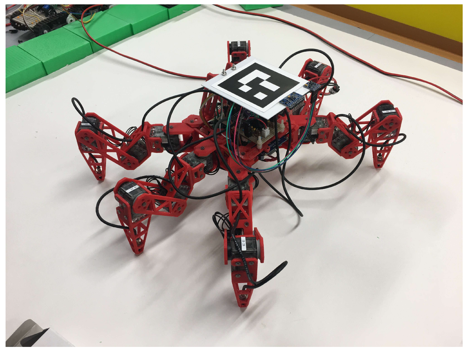
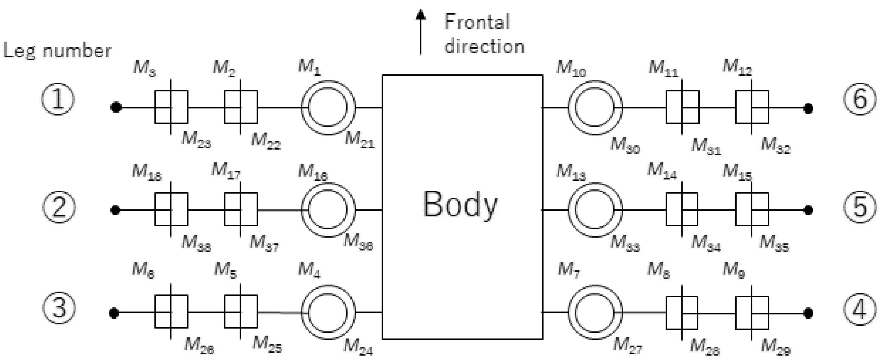
In this experiment, a physical calculation simulator and actual small multi-legged robot were adopted to evaluate the proposed method. Webots was used as a physical calculation simulator [19]. The virtual agent’s body was designed to be multi-legged, as shown in Figure 2. The virtual agent was compatible with the actual multi-legged robots that were developed for this experiment, as shown in Figure 3. The robot in Figure 3 is called Robot 1 hereinafter. The virtual agent and Robot 1 have 18 joints, and each joint is connected by a link, as shown in Figure 4. Obtaining the contact and posture information in the computer simulation is straightforward. However, Robot 1 needs to be equipped with sensors to obtain this information. Therefore, a touch sensor was implemented for the end point of each leg, and a gyro sensor was implemented on the robot’s body. In this configuration, the touch sensor can detect contact between the end point of the leg and the ground as on/off. To detect contact between the body and the ground, a laser distance sensor was implemented under the body.

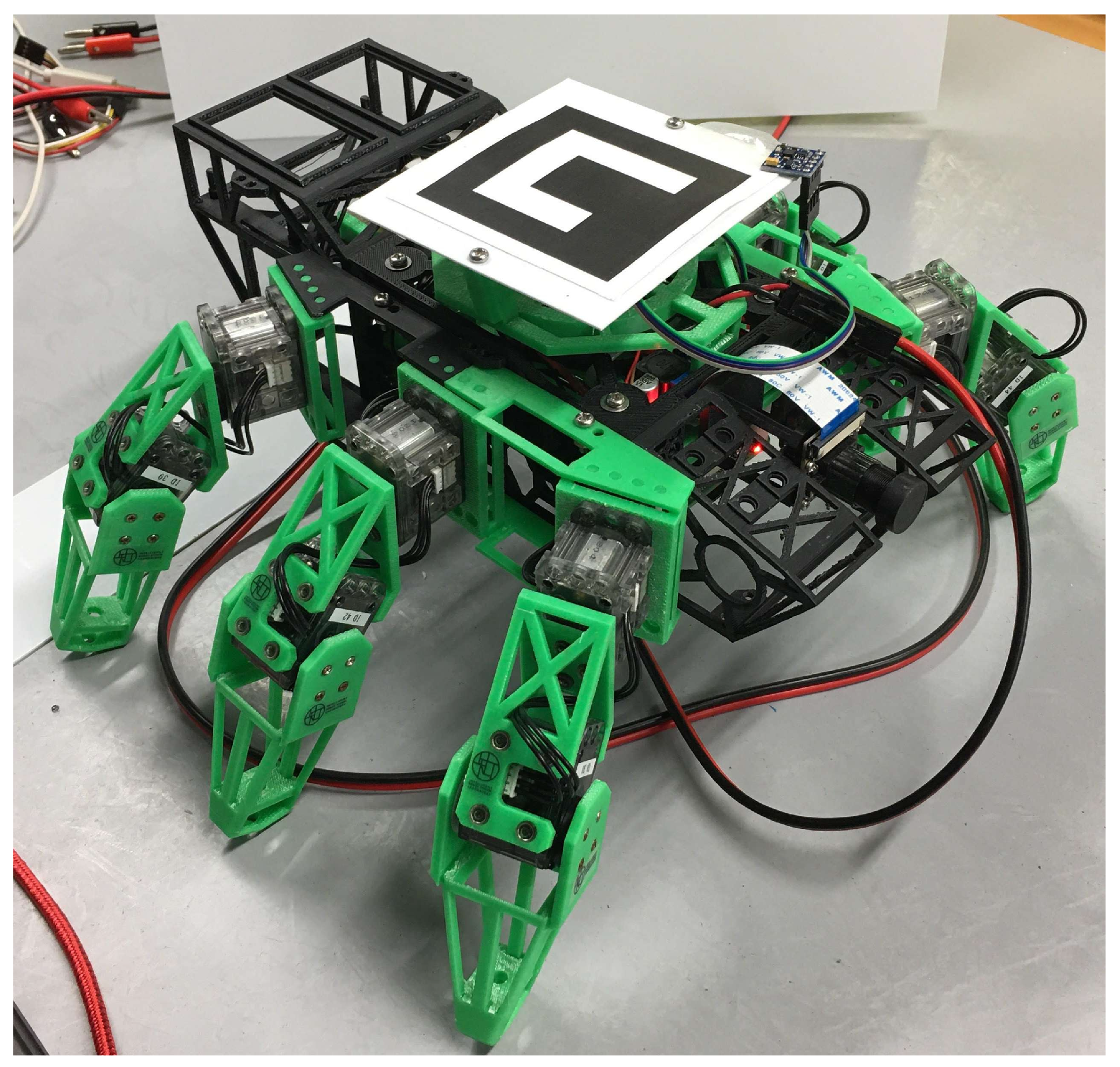
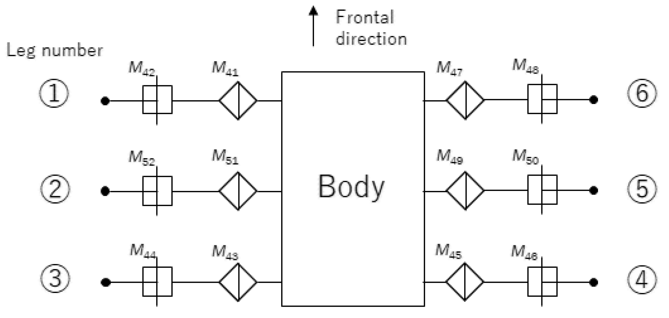
A different type of robot embodiment is shown in Figure 5, and this robot’s joint structure is shown in Figure 6. The robot in Figure 5 is called Robot 2. Robot 2 was also developed for this experiment. The specifications of the joints, sensors, and controls are the same as in Robot 1. Only the number of joints and the rotation angles of the joints are different from those of Robot 1. In Figure 4 and Figure 6, the motor IDs assigned to the virtual agent, Robot 1, and Robot 2 are $M_1$ to $M_{18}$, $M_{21}$ to $M_{38}$, and $M_{41}$ to $M_{52}$, respectively.

To obtain the self-coordination of the robot, actual robots have a marker on the top of body, as shown in Figure 3 and Figure 5. A camera for recognizing markers was implemented on the ceiling of the experimental environment. The self-position recognition server was installed outside, and the robots can acquire the self-coordinates from the server using a wireless LAN. When the agent and robot are controlled by the RL algorithm, the legs are actuated three legs at a time. For example, legs 1, 3, and 5 in Figure 4 move simultaneously with respect to the command value to rotate the joint. This contributes to a reduction of the action space and a simplification of control.

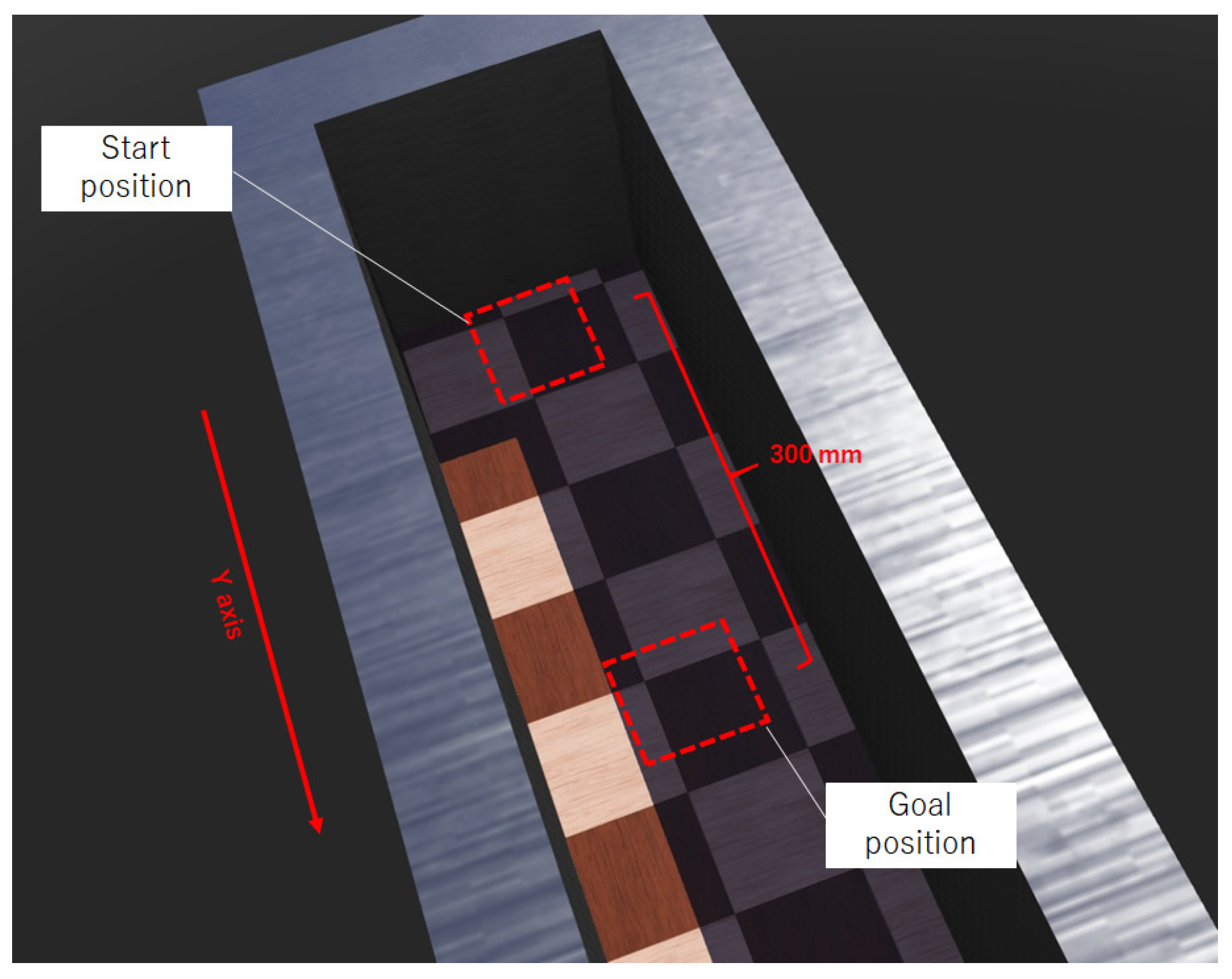
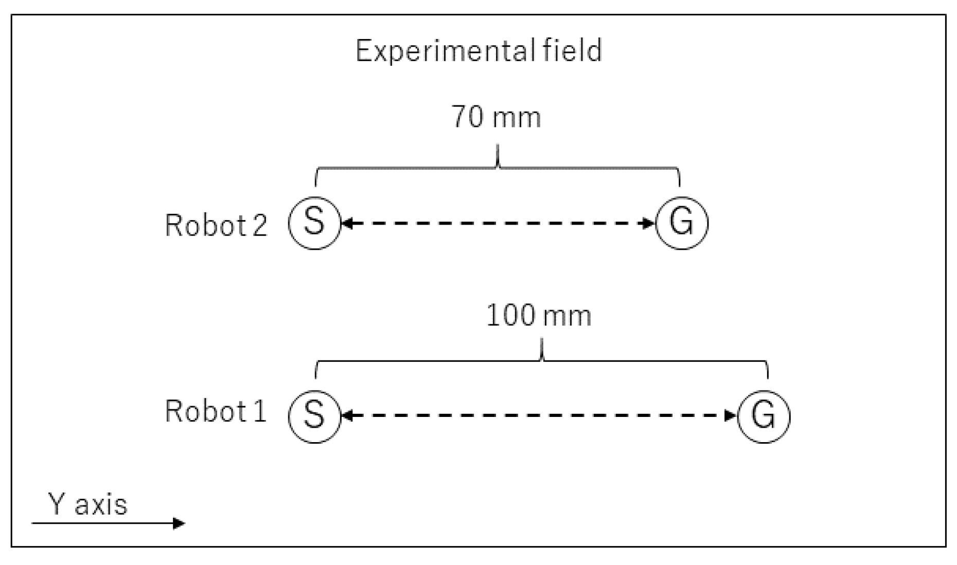
The virtual learning environment in Webots is constructed as shown in Figure 7. The distance between the starting and goal points was 300 mm. A wall was set around the experimental field, as shown in Figure 8, to give a negative reward to the agent. If the agent reached the goal, the agent’s position was automatically reset to the start position. The start position on the y-axis was the same, but the goal position differed depending on the robots, because each robot has a different maximum movement distance for one action. In the case of two robots, the goal position was set as the position reached by the same number of actions. If the robots reached the goal, the robots’ positions were reset to the start position by the human operator.

4.2. Conditions

At the beginning of this experiment, the moving behavior was learned through RL in Webots using a virtual agent. The parameters for RL were set as shown in

Table 1. Reinforcement learning parameters in simulation. These parameters are used for learning simulation in Webots.

Parameters	Values
Number of trials	5
Maximum number of episodes	100,000
Learning rate $\alpha$	0.1
Discount rate $\gamma$	0.99
Reward at reaching goal r	10
Reward per step $r_s$	−0.05
Reward for body contact with ground $r_g$	−0.1
Temperature of Boltzmann selection T	0.1

. After the learning of the simulation, the body calibration was executed using all agents and robots. In the experiment involving the robot, the parameters were the same as those given in Table 1, except that the maximum number of episodes was different because, unlike simulations, actual robots cannot perform the same number of episodes.

In the reward design, when the agent and robots reach the goal, the virtual agent and robots obtain a positive reward value of $r=10$, and therefore receive a negative reward value of $r_s=-0.05$ per step of an action. In addition, if the virtual agent and the robots’ bodies are in contact with the ground, they also obtain a negative reward value of $r_g=-0.1$. As an evaluation of the proposed method, the difference between the results from the proposed method and hand-coded inter-task mapping by a human who was not related to this study were compared. The evaluating factor used was the number of steps between the start and goal positions. Essentially, the smaller the number of steps, the higher the performance at the end of the learning process.

In this experiment, state $s\in S$ for RL and TL is defined as follows:

$$s=(x,y)\top .$$

(23)

In the robots, the above coordinates were set from the camera system described in Section 4.1, and for the agents, they could be obtained from Webots. The action $a\in A$ for RL and TL is defined as follows:

$$a=(M_i,M_j,M_k,\theta ).$$

(24)

Here, $M_x$ is the motor ID, and $i\ne j\ne k$ are the other IDs. The action a specifies the operation of the three servo motors and executes the changing angle command value of $\theta$ for each motor, where $\theta$ can be set as $+20$ degrees or $-20$ degrees from the current angle in this experimental condition.

4.3. Results of Learning Simulation

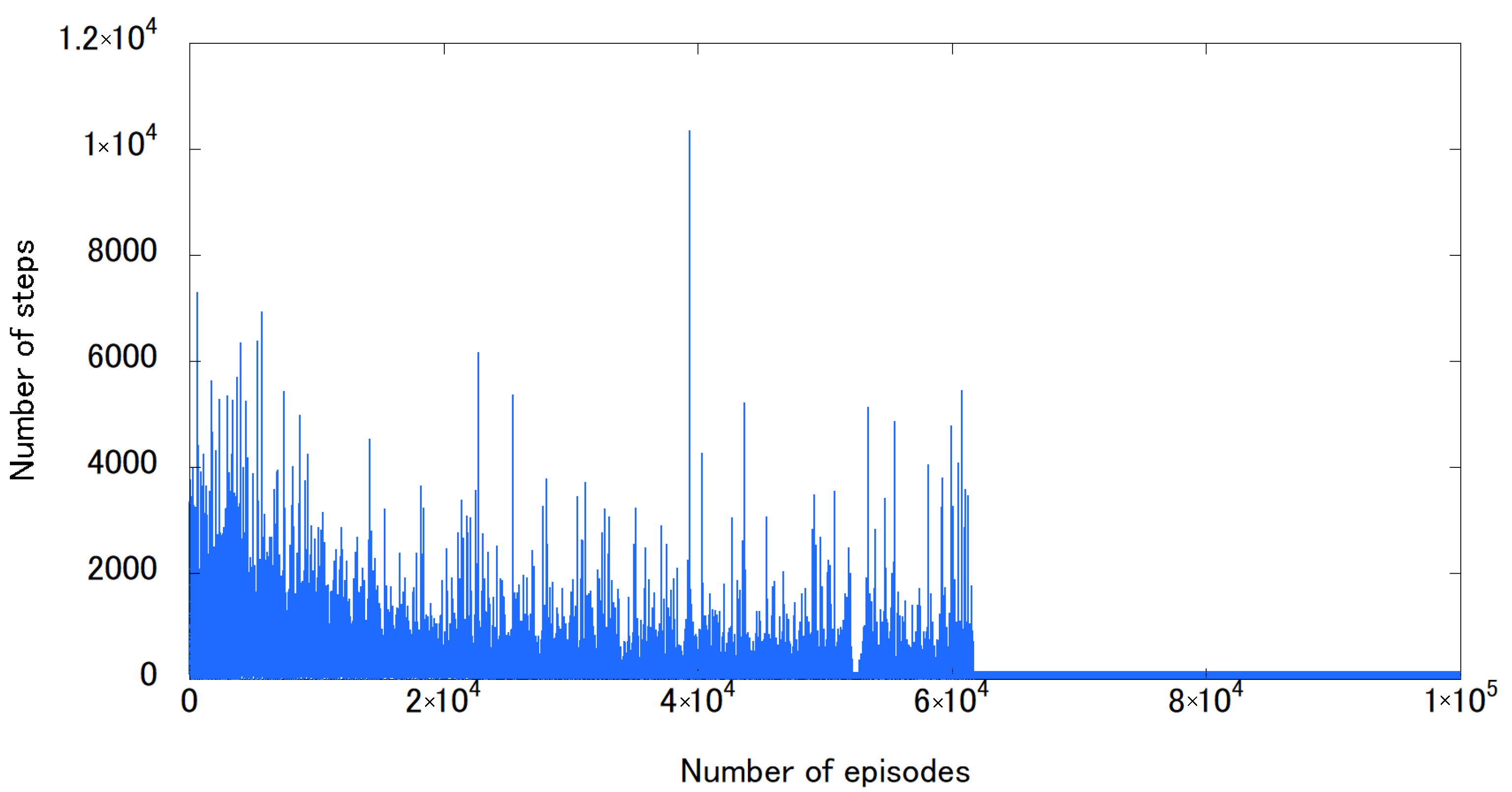
The results of the learning curve with a learning simulation of virtual agents are shown in Figure 9. In this figure, the learning curve converges at around 60,000 episodes. As for to general RL effects, the learning curve has a large number of steps at the beginning of learning, and the number of steps decreases with each episode. The virtual agent can be moved from the starting position to the goal with a gait motion.

4.4. Results for Body Calibration

Before transferring the obtained action-value function from the virtual agent to the actual robots, the results of the body calibration in the virtual agent and the robots are shown in

Table 2. Results of body calibration in virtual agent. This agent has motor IDs $M_1$ to $M_{18}$.

Action No. ${\mathit{a}}_{\mathit{i}}$, Motor IDs ${\mathit{M}}_{\mathit{j}}$, and Number of Executed Actions ${\mathit{n}}_{\mathit{k}}$	Body Vector ${\overline{\mathit{B}}}_{\mathit{i}}$	Foot Vector ${\overline{\mathit{F}}}_{\mathit{i}}$
($0,M_1,M_4,M_{13},100$)	$(-1.41\times {10}^{-2},-1.14\times {10}^{-5},1.15\times {10}^{-3})\top$	$(0,0,0,0,0,0)\top$
($1,M_1,M_4,M_{13},100$)	$(1.41\times {10}^{-2},-2.98\times {10}^{-6},1.25\times {10}^{-3})\top$	$(0,0,0,0,0,0)\top$
($2,M_{16},M_{10},M_7,100$)	$(1.41\times {10}^{-2},-3.00\times {10}^{-6},-1.20\times {10}^{-3})\top$	$(0,0,0,0,0,0)\top$
($3,M_{16},M_{10},M_7,100$)	$(-1.41\times {10}^{-2},-2.98\times {10}^{-6},1.25\times {10}^{-3})\top$	$(0,0,0,0,0,0)\top$
($4,M_{17},M_{11},M_8,100$)	$(-3.33\times {10}^{-5},2.81\times {10}^{-2},-1.38\times {10}^{-2})\top$	$(-2,-2,-2,0,0,0)\top$
($5,M_{17},M_{11},M_8,100$)	$(2.27\times {10}^{-9},-3.00\times {10}^{-4},-7.33\times {10}^{-5})\top$	$(0,0,0,-2,-2,-2)\top$
($6,M_{14},M_2,M_5,100$)	$(-1.41\times {10}^{-7},-2.95\times {10}^{-4},6.31\times {10}^{-5})\top$	$(-2,-2,-2,0,0,0)\top$
($7,M_{14},M_2,M_5,100$)	$(8.07\times {10}^{-5},2.81\times {10}^{-2},1.38\times {10}^{-2})\top$	$(0,0,0,-2,-2,-2)\top$
($8,M_{12},M_{18},M_9,100$)	$(-3.97\times {10}^{-5},-3.93\times {10}^{-4},-2.57\times {10}^{-3})\top$	$(0,0,0,-2,-2,-2)\top$
($9,M_{12},M_{18},M_9,100$)	$(3.94\times {10}^{-5},-4.09\times {10}^{-4},2.24\times {10}^{-3})\top$	$(0,0,0,-2,-2,-2)\top$
($10,M_{15},M_3,M_6,100$)	$(3.73\times {10}^{-5},-4.04\times {10}^{-4},2.56\times {10}^{-3})\top$	$(-2,-2,-2,0,0,0)\top$
($11,M_{15},M_3,M_6,100$)	$(-3.77\times {10}^{-5},-4.09\times {10}^{-4},-2.24\times {10}^{-3})\top$	$(-2,-2,-2,0,0,0)\top$

,

Table 3. Results of body calibration in Robot 1. This robot has motor IDs $M_{21}$ to $M_{38}$.

Action No. ${\mathit{a}}_{\mathit{i}}$, Motor IDs ${\mathit{M}}_{\mathit{j}}$, and Number of Executed Actions ${\mathit{n}}_{\mathit{k}}$	Body Vector ${\overline{\mathit{B}}}_{\mathit{i}}$	Foot Vector ${\overline{\mathit{F}}}_{\mathit{i}}$
($0,M_{21},M_{24},M_{34},1$)	$(-1.11\times {10}^{-2},-8.36\times {10}^{-4}-2.38\times {10}^{-2})\top$	$(0,0,0,0,0,0)\top$
($1,M_{21},M_{24},M_{33},1$)	$(7.45\times {10}^{-3},2.33\times {10}^{-3},-1.87\times {10}^{-2})\top$	$(0,0,0,0,0,0)\top$
($2,M_{36},M_{27},M_{30},1$)	$(7.19\times {10}^{-3},4.70\times {10}^{-4},1.40\times {10}^{-2})\top$	$(0,0,0,0,0,0)\top$
($3,M_{26},M_{27},M_{30},1$)	$(-7.33\times {10}^{-3},4.07\times {10}^{-4},-1.40\times {10}^{-2})\top$	$(0,0,0,0,0,0)\top$
($4,M_{31},M_{37},M_{28},1$)	$(-4.98\times {10}^{-3},9.84\times {10}^{-3},-9.43\times {10}^{-3})\top$	$(0,0,0,-2,-2,-2)\top$
($5,M_{31},M_{37},M_{28},1$)	$(-2.41\times {10}^{-3},-2.45\times {10}^{-3},6.81\times {10}^{-5})\top$	$(0,-3,-3,0,0,0)\top$
($6,M_{25},M_{34},M_{22},1$)	$(1.36\times {10}^{-4},-4.00\times {10}^{-3},5.48\times {10}^{-6})\top$	$(0,0,0,-2,-2,-2)\top$
($7,M_{25},M_{34},M_{22},1$)	$(-4.64\times {10}^{-3},6.88\times {10}^{-3},-9.53\times {10}^{-3})\top$	$(-6,0,0,0,0,0)\top$
($8,M_{32},M_{38},M_{29},1$)	$(2.52\times {10}^{-6},-5.00\times {10}^{-4},4.92\times {10}^{-7})\top$	$(0,0,0,0,0,0)\top$
($9,M_{32},M_{38},M_{29},1$)	$(-4.56\times {10}^{-5},-3.50\times {10}^{-3},9.85\times {10}^{-5})\top$	$(0,-3,-3,0,0,0)\top$
($10,M_{23},M_{35},M_{26},1$)	$(2.41\times {10}^{-3},2.55\times {10}^{-3},-4.65\times {10}^{-3})\top$	$(0,0,0,0,0,0)\top$
($11,M_{23},M_{35},M_{26},1$)	$(2.61\times {10}^{-3},-5.33\times {10}^{-3},4.76\times {10}^{-3})\top$	$(0,0,0,-2,-2,-2)\top$

and

Table 4. Results of body calibration in Robot 2. This robot has motor IDs $M_{41}$ to $M_{52}$.

Action No. ${\mathit{a}}_{\mathit{i}}$, Motor IDs ${\mathit{M}}_{\mathit{j}}$, and Number of Executed Actions ${\mathit{n}}_{\mathit{k}}$	Body Vector ${\overline{\mathit{B}}}_{\mathit{i}}$	Foot Vector ${\overline{\mathit{F}}}_{\mathit{i}}$
($0,M_{43},M_{41},M_{49},100$)	$(-2.35\times {10}^{-3},6.32\times {10}^{-5},4.70\times {10}^{-3})\top$	$(0,0,0,-2,-2,-2)\top$
($1,M_{43},M_{41},M_{49},100$)	$(2.36\times {10}^{-3},-1.48\times {10}^{-3},4.64\times {10}^{-3})\top$	$(0,0,0,-2,-2,-2)\top$
($2,M_{51},M_{47},M_{45},100$)	$(-2.33\times {10}^{-3},1.91\times {10}^{-4},-4.71\times {10}^{-3})\top$	$(-2,-2,-2,0,0,0)\top$
($3,M_{51},M_{47},M_{45},100$)	$(2.30\times {10}^{-3},-2.42\times {10}^{-3},4.77\times {10}^{-3})\top$	$(-2,-2,-2,0,0,0)\top$
($4,M_{52},M_{48},M_{1}46,100$)	$(3.32\times {10}^{-5},-8.72\times {10}^{-4},-4.68\times {10}^{-3})\top$	$(-2,-2,-2,0,0,0)\top$
($5,M_{52},M_{48},M_{1}46,100$)	$(-2.38\times {10}^{-3},-2.22\times {10}^{-3},9.05\times {10}^{-5})\top$	$(0,0,0,-2,-2,-2)\top$
($6,M_{50},M_{42},M_{44},100$)	$(1.17\times {10}^{-5},-3.25\times {10}^{-3},-8.54\times {10}^{-6})\top$	$(-2,-2,-2,0,0,0)\top$
($7,M_{50},M_{42},M_{44},100$)	$(9.86\times {10}^{-5},-1.78\times {10}^{-3},-4.79\times {10}^{-3})\top$	$(0,0,0,-3,0,-3)\top$

. The tables show the calculation results of the body diagram corresponding to the action number. The corresponding motor ID is attached to the action number, giving a correspondence table between the body ${\overline{\mathbf{B}}}_i$ and foot ${\overline{\mathbf{F}}}_i$ as a result of moving the motor. In these tables, the foot-vector values are indicated as negative values because all foot sensors are detected at the default position of the robot. Therefore, after an action, the change in the foot vector is a small value.

Table 5. Results of mapping using each body diagram and hand coding.

Action Number of Virtual Agent	Mapping to Robot 1 by Proposed Method	Mapping to Robot 1 by Hand Coding	Mapping to Robot 2 by Proposed Method	Mapping to Robot 2 by Hand Coding
0	0	0	0	0
1	1	1	1	1
2	2	2	7	2
3	3	3	6	3
4	7	4	4	N/M 4
5	6	5	5	N/M 4
6	5	6	N/M 4	N/M 4
7	4	7	N/M 4	N/M 4
8	11	8	N/M 4	4
9	10	9	N/M 4	5
10	9	10	3	6
11	8	11	2	7

⁴ N/M indicates that there is nothing to map.

shows the mapping results of body calibration. Between the virtual agent and Robot 2, there are cases where there is nothing to map because the DOF are different. In the case of mapping between the virtual agent and Robot 1, the DOF are the same but the mapping does not match exactly. The validity of this mapping result is verified by the results shown in the next subsection. In the next subsection, the action-value function obtained by simulation is transferred to an actual robot, and the behavior of the robot using the mapping obtained by this body calibration is described for the inter-task mapping of TL.

4.5. Results of Transfer to Robots

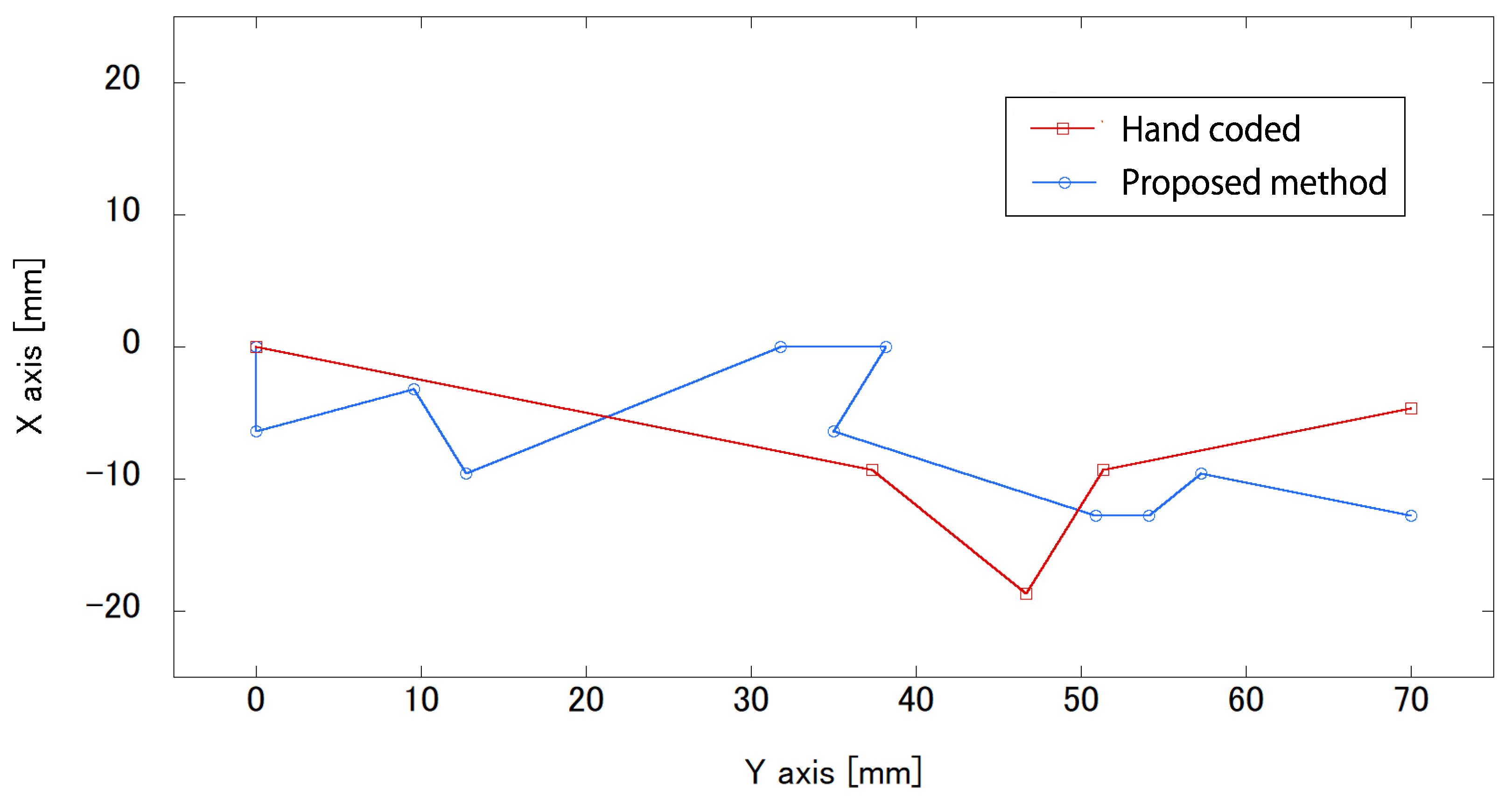
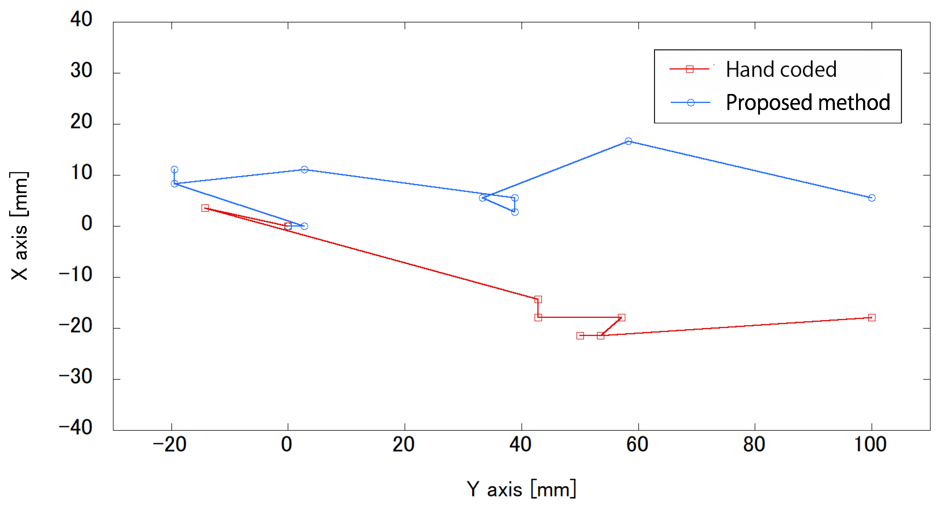
The results for the movement trajectory of Robot 1 are shown in Figure 10 and the movement trajectory of Robot 2 is shown in Figure 11. These movement trajectories are illustrations of experiments that were attempted five times for each robot. In the trajectories in the figures, the coordinates $(x,y)=(0,0)$ represent the starting position of the robot, based on the marker. The goal position is 70 mm along the y-axis in Figure 10. The goal position in Figure 11 is 100 mm along the y-axis.

For the trajectories of Robot 1, hand-coded conditions are needed to move in four steps from the starting position to the goal. However, the proposed method condition takes 33 steps to move from the starting position to the goal. In other trials, hand coding may require more steps. Both conditions in Figure 10 show that the task of moving forward and reaching the goal was accomplished. In the trajectories of Robot 2, it appears that there is no significant difference in the number of steps between the hand-coded method and the proposed method, and the task of moving forward and reaching the goal was accomplished, as in the experiment with Robot 1.

4.6. Discussion

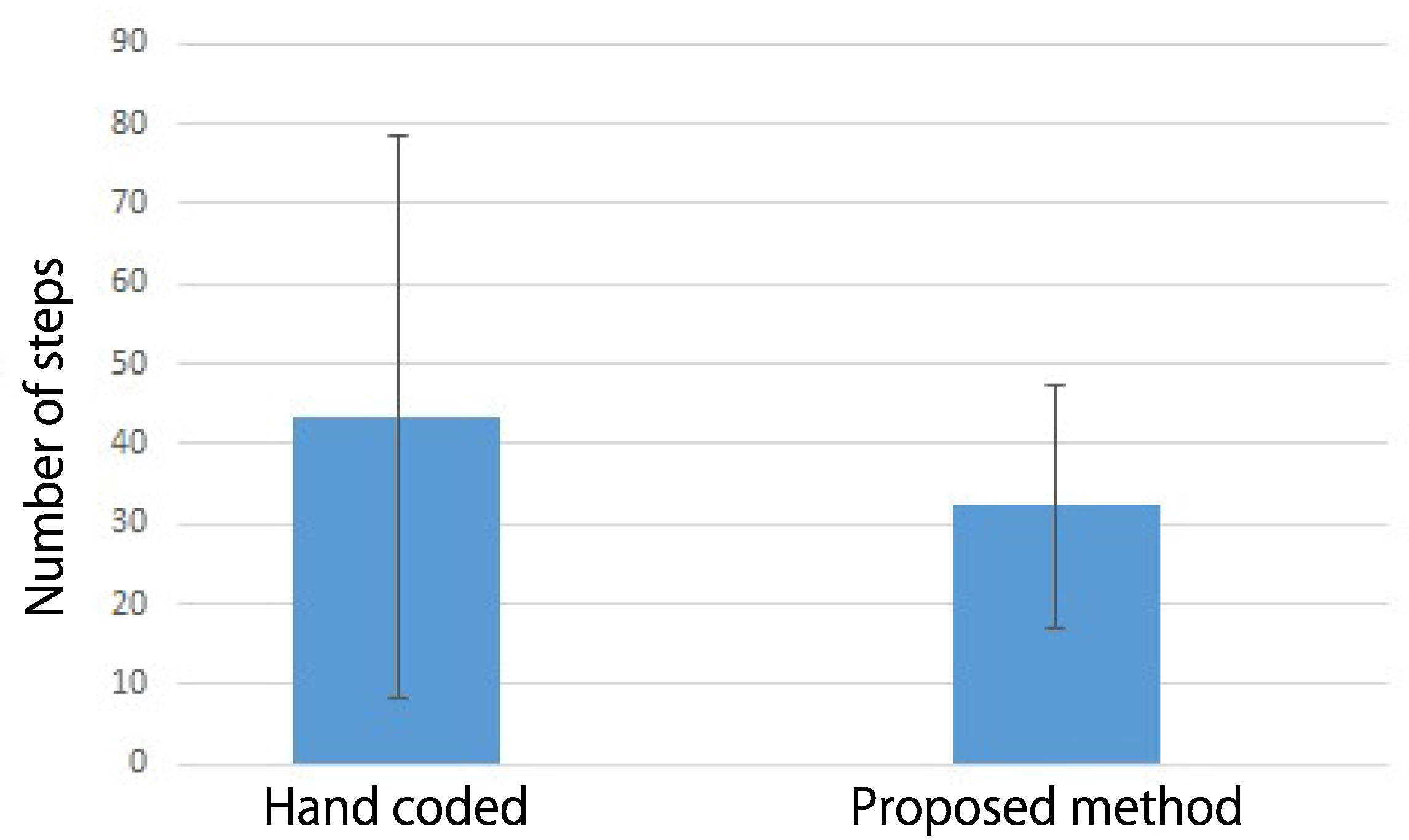
The averaged number of steps and the standard deviation for five trials are shown in Figure 12 and Figure 13. In Figure 12, the result using Robot 1 focuses on the average value. The hand-coded method and the proposed method have a similar number of steps, and there is no significant difference. However, since the deviation is smaller in the proposed method compared with the hand-coded method, it is suggested that it could be possible to avoid design mistakes by humans and maintain the performance of TL by automating the mapping using the proposed method. In this case, the virtual agent and Robot 1 have the same embodiments in terms of DOF and structure. In fact, the hand-coded mapping is intuitively correct because the action number of the virtual agent is mapped to the same action number in Robot 1. Nevertheless, the reason why the deviation in the number of steps is so large is assumed to be because there is a difference in the behavior of the virtual agents and robots in the simulation and real environments. This fact shows that the proposed method of body calibration can absorb and map the difference between the simulation and actual environments, even if the embodiments of the virtual agent and robot are the same.

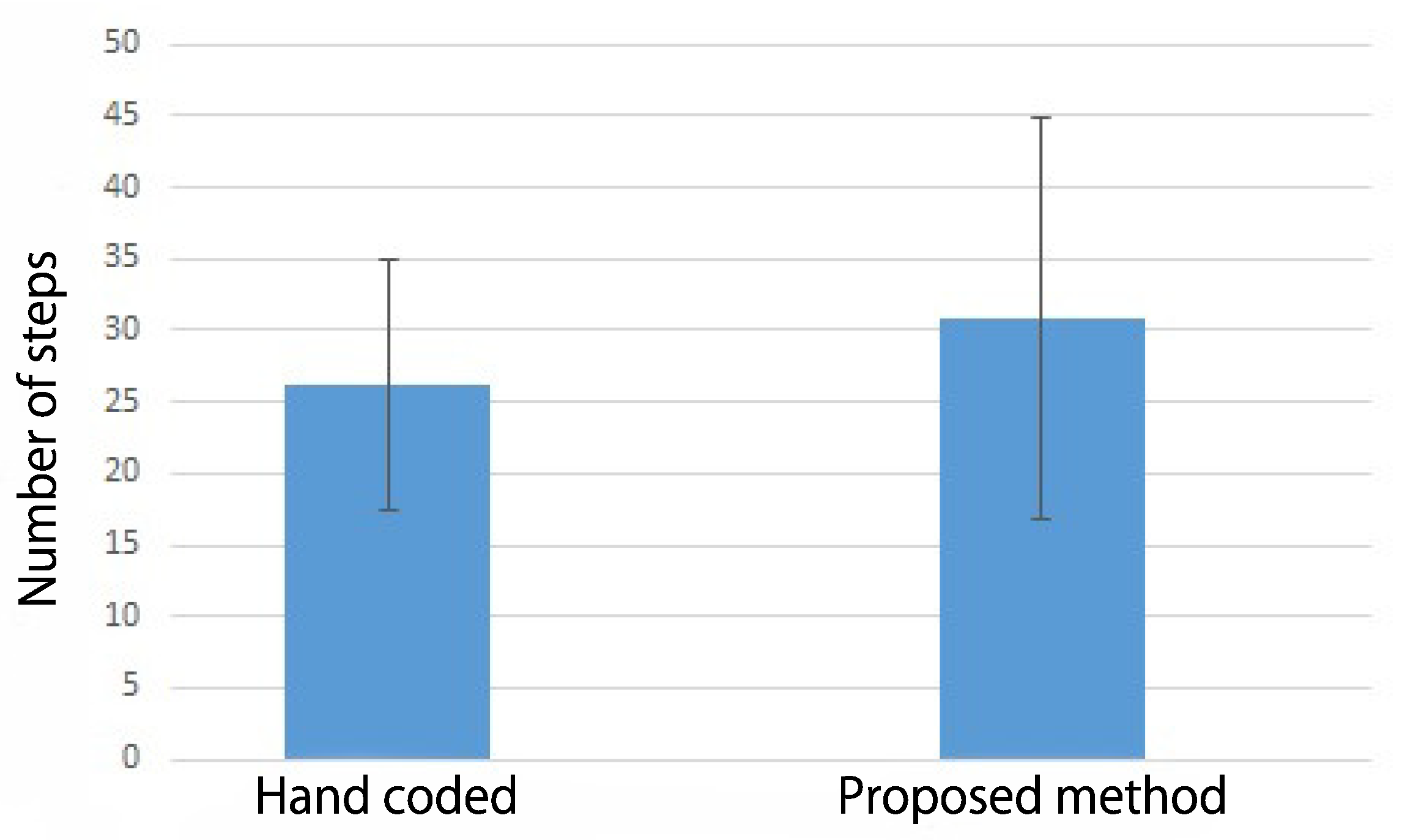
However, under the experimental condition using Robot 2, there is no large difference in the number of steps, as shown in Figure 12. Additionally, the deviation is larger in the proposed method than in the hand-coded method. Because the DOF of the robot at the transfer destination are fewer than those of the virtual agent, this may increase the difficulty of TL. Another reason for the deviation may be the differences from the simulation when the real robot interacts with the real environment, e.g., slip and control errors.

The difficulty level of TL also changes depending on the differences in the embodiments of agents and robots. Therefore, although the effect of the proposed method has changed, the experimental results indicate that the mapping can be automated, because there is no large difference in the transfer results between the proposed and hand-coded methods. However, the standard deviation of the experimental results is large overall. This is because the gait motion has not been sufficiently acquired in the RL process. In this experiment, reaching the destination is the main reward condition of RL, and therefore gait efficiency and load are not taken into consideration. Therefore, execution of the policy obtained in the simulation put a load on the joints motors of the actual robot. It is considered that the number of actions to reach the goal became unstable and the standard deviation of the number of steps became large.

5. Conclusions

This study proposed an automatic inter-task mapping method for transfer reinforcement learning inspired by the body representation in the human brain. Body calibration using a body diagram calculated using body and foot vectors was proposed and evaluated using learning simulation and actual robots. Before the transfer of knowledge to actual robots, the behavior was learned with RL using a virtual agent which contained 18 actuators operating six legs in a multi-legged robot. After the simulation, the obtained action-value function was transferred to the actual robot, and the robot moved using the obtained action-value functions through body diagrams which were obtained by body calibration. As a result, compared with human-designed inter-task mapping, the TL using body diagrams had the same effect as the TL for which the mapping was set manually. Therefore, automatic inter-task mapping was realized. In addition, this result shows that the proposed method, body calibration, could absorb and map the differences between the simulation and actual environments, even if the embodiment of the virtual agent and robot were the same.

In future work, it will be necessary to evaluate the usefulness of the proposed method using a robot with a different embodiment, as well as investigating the difficulty of transfer and experimental conditions with extremely different DOF. Moreover, under the experimental conditions of this paper, the movement distance of the robot was at the most 100 mm, and therefore it is necessary to evaluate the method by moving a longer distance and measuring the effect in a more complicated environmental shape. It is also important to measure the limits of the proposed method. In addition, the effect of the transfer depends on the difference between the simulation and the actual experiment; therefore, the performance of the proposed method also depends on this difference. It is necessary to clarify the differences in the effects of TL owing to the differences between the simulation and actual experiments and the relationship between the effects in the proposed method. Considering the implementation in real applications, it is necessary to evaluate the accuracy of the method and verify the real-time property.

References

1. Sutton, R.S.; Barto, A.G. Reinforcement Learning: An Introduction; The MIT Press: Cambridge, MA, USA, 1998. [Google Scholar]
2. Kober, J.; Bagnell, J.A.; Peters, J. Reinforcement learning in robotics: A survey. Int. J. Robot. Res. 2013, 32, 1238–1274. [Google Scholar] [CrossRef] [Green Version]
3. Taylor, M.E. Transfer in Reinforcement Learning Domains; Ser. Studies in Computational Intelligence; Springer: Berlin/Heidelberg, Germany, 2009; p. 216. [Google Scholar]
4. Lazaric, A. Reinforcement Learning—State of the art. In Transfer in Reinforcement Learning: A Framework and A Survey; Springer: Berlin/Heidelberg, Germany, 2012; Volume 12, pp. 143–173. [Google Scholar]
5. Kono, H.; Murata, Y.; Kamimura, A.; Tomita, K.; Suzuki, T. Transfer Learning Method Using Ontology for Heterogeneous Multi-agent Reinforcement Learning. Int. J. Adv. Comput. Sci. Appl. 2014, 5, 15–164. [Google Scholar] [CrossRef] [Green Version]
6. Taylor, M.E.; Kuhlmann, G.; Stone, P. Autonomous transfer for reinforcement learning. In Proceedings of the Seventh International Joint Conference on Autonomous Agents and Multiagent Systems, Estoril, Portugal, 12–16 May 2008; pp. 283–290. [Google Scholar]
7. Fachantidis, A.; Partalas, I.; Taylor, M.E.; Vlahavas, I. Transfer learning with probabilistic mapping selection. Adapt. Behav. 2015, 23, 3–19. [Google Scholar] [CrossRef] [Green Version]
8. Cheng, Q.; Wang, X.; Shen, L. An Autonomous Inter-task Mapping Learning Method via Artificial Network for Transfer Learning. In Proceedings of the IEEE International Conference on Robotics and Biomimetics, Macau, China, 5–8 December 2017; pp. 768–773. [Google Scholar]
9. Mnih, V.; Kavukcuoglu, K.; Silver, D.; Rusu, A.A.; Veness, J.; Bellemare, M.G.; Graves, A.; Riedmiller, M.; Fidjel, A.K.; Ostrovski, G.; et al. Human-Level control through deep reinforcement learning. Nature 2015, 518, 529–533. [Google Scholar] [CrossRef]
10. Hou, Y.; Ong, Y.; Feng, L.; Zurada, J.M. An Evolutionary Transfer Reinforcement Learning Framework for Multiagent Systems. IEEE Trans. Evol. Comput. 2017, 21, 601–615. [Google Scholar] [CrossRef]
11. Peng, X.B.; Coumans, E.; Zhang, T.; Lee, T.-W.E.; Tan, J.; Levine, S. Learning Agile Robotic Locomotion Skills by Imitating Animals. In Proceedings of the Robotics: Science and Systems, Corvalis, OR, USA, 12–16 July 2020. [Google Scholar]
12. Kono, H.; Katayama, R.; Takakuwa, Y.; Wen, W.; Suzuki, T. Activation and Spreading Sequence for Spreading Activation Policy Selection Method in Transfer Reinforcement Learning. Int. J. Adv. Comput. Sci. Appl. 2019, 10, 7–16. [Google Scholar] [CrossRef]
13. Ota, J. Understanding Brain Plasticity on Body Representations to Promote Their Adaptive Functions; 2018 Annual Report; Kaken: Tokyo, Japan, 2018. [Google Scholar]
14. Wen, W.; Katsutoshi, M.; Shunsuke, H.; Qi, A.; Hiroshi, Y.; Yusuke, T.; Atsushi, Y.; Hajime, A. Goal-Directed Movement Enhances Body Representation Updating. Front. Hum. Neurosci. 2016, 10, 1–10. [Google Scholar] [CrossRef] [PubMed] [Green Version]
15. Watkins, C.J.C.H.; Dayan, P. Q-Learning. Mach. Learn. 1992, 8, 279–292. [Google Scholar] [CrossRef]
16. Peng, X.B.; Andrychowicz, M.; Zaremba, W.; Abbeel, P. Sim-to-Real Transfer of Robotic Control with Dynamics Randomization. In Proceedings of the 2018 IEEE International Conference on Robotics and Automation, Brisbane, Australia, 21–25 May 2018; pp. 3803–3810. [Google Scholar]
17. Baar, J.V.; Sullivan, A.; Cordorel, R.; Jha, D.; Romeres, D.; Nikovski, D. Sim–to–Real Transfer Learning using Robustified Controllers in Robotic Tasks involving Complex Dynamics. In Proceedings of the 2019 International Conference on Robotics and Automation (ICRA), Montreal, QC, Canada, 20–24 May 2019; pp. 6001–6007. [Google Scholar]
18. Hwasser, M.; Kragic, D.; Antonova, R. Variational Auto-Regularized Alignment for Sim–to–Real Control. In Proceedings of the 2020 IEEE International Conference on Robotics and Automation (ICRA), Paris, France, 31 May–31 August 2020; pp. 2732–2738. [Google Scholar]
19. Webots: Open Source Robot Simulator. Available online: https://cyberbotics.com/ (accessed on 30 January 2022).
20. ROBOTIS: Dynamixel XL-320. Available online: https://www.robotis.us/dynamixel-xl-320/ (accessed on 30 January 2022).
Figure 1. Simplified illustration of proposed method. The right side explains traditional transfer reinforcement learning, and the left side explains body calibration’s information flow.
Actuators 11 00140 g001
Figure 2. Multi-legged type of virtual agent in Webots. Scales such as for the lengths of the links and the positions of joints and the body are set to be similar to those of an actual robot, as shown in Figure 3. This model is controlled by a Python program in Webots, and information on contact between the ground and the end point of a leg can be obtained in the program.
Actuators 11 00140 g002
Figure 3. Actual multi-legged robot (called Robot 1). All the joints are realized using a servo motor, and the link and body structures are generated using a 3D printer. All the motors and sensors are controlled and connected using a Raspberry Pi, which is powered by a small LiPO battery. This robot also drives an external power source using a regulated DC power supply device. The servo motor used was a Dynamixel XL-320 [20], and the Python library Pypot was used to control the servo motor through the U2D2 module from the Raspberry Pi.
Actuators 11 00140 g003
Figure 4. Joint placement and structure of Robot 1 in top view. All the joints are rotational joints. The end point of each leg has a touch sensor, as described above. Leg numbers are assigned in this figure, for the control. Motor IDs M 1 to M 18 are assigned to the virtual agent, and motor IDs M 21 to M 38 are assigned to Robot 1.
Actuators 11 00140 g004
Figure 5. Different robot embodiment. The system configuration for elements such as servo motors and touch sensors is the same as in Robot 1. Only the number of joints and rotation angles of the joints are different from Robot 1.
Actuators 11 00140 g005
Figure 6. Joint placement and structure of Robot 2 in a top view. Motor IDs M 41 to M 52 are assigned to Robot 2.
Actuators 11 00140 g006
Figure 7. Virtual environment in Webots. In this figure, the distance between the start and goal position is 300 mm. The agent has learned the motion of the legs to begin moving towards the goal.
Actuators 11 00140 g007
Figure 8. Simplified overview of the actual learning environment. This figure is a bird’s-eye view. S denotes the start position and G denotes the goal position.
Actuators 11 00140 g008
Figure 9. Learning curve obtained from learning simulation with virtual agents. The x-axis denotes the number of episodes, indicating the iteration number of learning. The y-axis denotes the number of steps between the start and goal positions. In other words, the number of steps represents the problem-solving time or number of action selections.
Actuators 11 00140 g009
Figure 10. Movement trajectory of Robot 1 when the action-value function is transferred from the virtual agent through body calibration. As a comparison, the movement trajectory of Robot 1 during the transfer of learning using hand-coded inter-task mapping is used.
Actuators 11 00140 g010
Figure 11. Movement trajectory of Robot 2 when the action-value function is transferred from the virtual agent through body calibration. As a comparison, the movement trajectory of Robot 2 during the transfer of learning using hand-coded inter-task mapping is used.
Actuators 11 00140 g011
Figure 12. Averaged number of steps and standard deviation over five trials ( n = 5 ) in Robot 1, for comparison between the proposed and hand-coded methods.
Actuators 11 00140 g012
Figure 13. Averaged number of steps and standard deviation over five trials ( n = 5 ) in Robot 2, for comparison between the proposed and hand-coded methods.
Actuators 11 00140 g013