1. Introduction
Condensers are essential heat-transfer equipment [
1] in petrochemical and power plant industries. The current cleaning methods for these are mostly tandem robotic arms or manually operated high-pressure water-gun cleaning [
2,
3]. However, high-pressure water backlash and other factors cause the existing methods to be less stable, accurate, and efficient than is desired, and special cleaning robots must be developed for the use of condensers.
Kinematic and dynamic analyses are the basis for parallel mechanism research [
4,
5,
6]. Lei et al. [
7] conducted kinematics calibration and error analysis for a 3-RRRU parallel robot, while Jinzhu et al. [
8] proposed a multi-branch coupled parallel drive mechanism with five degrees of freedom and analysed the mechanism based on the azimuth feature set method, degrees of freedom, and motion characteristics of the end of the mechanism. The existing dynamic modeling methods mainly include: the Newton–Euler method [
9,
10,
11], Lagrangian method [
12,
13], and virtual work principle method [
14,
15,
16], in which the virtual work principle omits calculation constraints force and moment, and the derivation process is concise. Xinxue et al. [
17] conducted a singular analysis of the 2-UPR-RPU parallel mechanism, while Guangchun et al. [
18] used the virtual work principle to carry out dynamic and power analyses. The PD/PID control method is usually used to control the trajectory and pose of the parallel mechanism [
19,
20,
21], but control will be affected by the parameter error or external load disturbance in the dynamic model of the parallel mechanism. Xuemei et al. [
22] used ASMC to suppress the load disturbance of the parallel mechanism but did not consider the parameter uncertainty and the time-varying load. Navabi [
23] combined SMC with a fuzzy system to improve the uncertainty of structural and non-structural parameters and controller performance. Zhang Bin et al. [
24] proposed a dual-space adaptive synchronisation controller, which could significantly improve the control accuracy of the moving platform. Liu et al. [
25] proposed a terminal sliding mode-based control strategy to achieve accurate motion tracking control. Liu Yu et al. [
26] proposed an I&I controller that estimated the interference error in real-time based on the adaptive law, designing the control rate through the sliding surface, which realised the pose control of the robot. Long et al. [
27] proposed an ASMC method with an RBFNN compensator and Newton–Eulerian estimator to achieve real-time attitude control.
The working mechanism of cleaning robots is as follows. First, the mouth of the tube bundle is located using the vision system. Second, the parallel mechanism and the gun feeding device cooperate for pose adjustment, which, however, is disturbed by the backlash of high-pressure water, thereby affecting the cleaning effect.
In this paper, a hybrid robot with a redundant mechanism is designed. The variation, velocity, and acceleration model of each rod of the 4-RPU mechanism are obtained through the inverse kinematics solution, and the dynamic model of the mechanism is constructed using the principle of virtual work. Considering the parameter error of the model and external load disturbance, an adaptive law based on sliding mode surface construction is used to estimate and compensate for this uncertainty, and an adaptive sliding mode control method is proposed, which has a simple structure and can accurately estimate and overcome the time variance. Compared with the traditional sliding mode control algorithm, the average tracking error is effectively reduced.
2. Description and Degree of Freedom Analysis
2.1. Institution Description
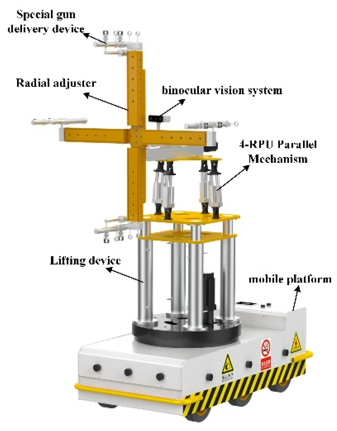
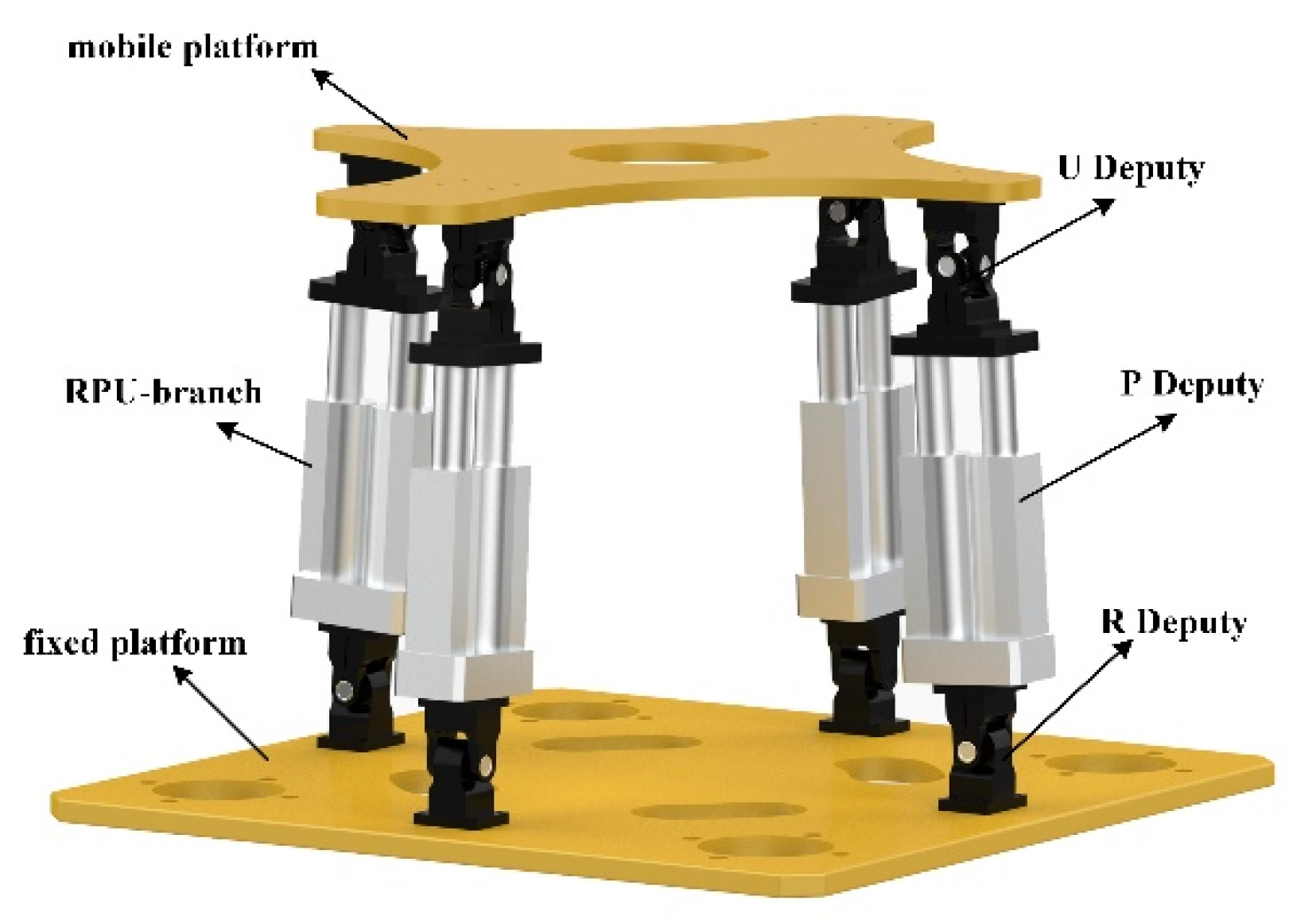
Figure 1 is a schematic structural diagram of a hybrid condenser cleaning robot, the function of which is to clean the dirt from the inner wall of the condenser tube bundle. It mainly includes a mobile platform, 4-RPU parallel mechanism, binocular vision system, and special gun feeding device. Through the parallel mechanism, the working attitude of the special gun feeding device can be adjusted. As shown in
Figure 2, the 4-RPU parallel mechanism is composed of a fixed platform, a moving platform, and four identical RPU (rotating pair-moving pair-Hooker hinge) branches. The branches are symmetrically distributed on the fixed platform. In the RPU symmetrical branch chain, the rotation axis of the R pair is parallel. The moving direction of the P pair passes through the center of the U pair and is always perpendicular to the rotation axis of the R pair. The first rotation axis of the U pair connected to the moving platform is parallel to the R pair axis, and the second axis by moving the platform centroid.
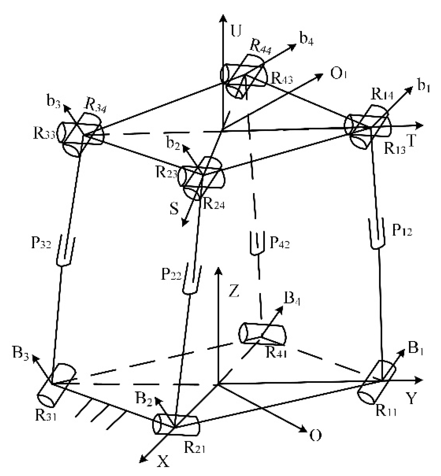
The 4-RPU parallel topology is shown in
Figure 3. B
1, B
2, B
3, and B
4 are the rotation center points of the R pair in the RPU branch chain, and b
1, b
2, b
3, and b
4 are the rotation center points of the U pair. The origin O of the fixed coordinate system is the center point of B
1B
3, the X-axis is collinear with OB
2, the Y-axis is along the direction of OB
1, and the Z-axis is determined by the right-hand rule to be vertically upward. The origin O
1 of the moving coordinate system is the center of mass of the moving platform, T is pointing to O
1b
1, S is along the direction of O
1b
2, and it can be determined that the U axis is vertical and the moving platform is upward.
2.2. Degree of Freedom Analysis
As shown in
Figure 3, the topology of the branch chain is as follows:
In the parallel regulation platform, the POC set of each branch end member is:
From the analysis of the topology structure, it can be seen that the parallel adjustment platform has three independent loops, and the number of independent displacement equations of the first independent loop is set as:
Let the number of independent displacement equations of the second independent loop then be:
Moreover, let the number of independent displacement equations of the third independent loop then be:
Through the above analysis, the degrees of freedom of the 4-RPU parallel mechanism are:
Combined with the judgment criteria of passive motion pairs in the parallel mechanism, it can be seen that there is no passive motion pair in the 4-RPU parallel mechanism. In Equation (6), the 4-RPU parallel mechanism has three degrees of freedom, including two rotations around the S axis, T axis, and movement along the U axis, including a redundant branch chain. From the analysis results of the degrees of freedom, the requirements of the condenser cleaning robot for posture adjustment during cleaning operations can be seen to be met.
3. Kinematic Analysis and Dynamic Modeling
3.1. Inverse Position Solution
The inverse position solution for the 4-RPU parallel mechanism determines the specific size parameters of the mechanism and the pose of the moving platform center O1 relative to the fixed coordinate system, determining the rod length vectors of the drive rods in each branch of the mechanism using the rotation matrix.
For a 4-RPU parallel mechanism, the rotation matrix of the moving coordinate system relative to the fixed coordinate system can be expressed as:
According to the movement degrees of freedom of the 4-RPU parallel platform, the attitude matrix of the moving coordinate system relative to the fixed coordinate system can be expressed as:
The third column of
is the unit vector
of the branch direction. As shown in
Figure 3, the vector equations of each motion branch of the 4-RPU parallel mechanism are established:
Let
,
,
, and
represent the position vectors of
,
,
, and
in the fixed/moving coordinate system, respectively.
According to the mechanism theory, the positions of the vector
and the rotation secondary axis vector
in the fixed coordinate system can be expressed as:
It can be seen from Formula (9) that the coordinate vector of the center point
O1 of the moving platform in the fixed coordinate system is
. By establishing the constraint equation, the secondary axis of rotation
d1 can be determined to always be perpendicular to the plane B
1b
1b
3B
3, and the relationship between X and Z obtained.
We can learn from
that the position of the origin of the moving coordinate system s in the fixed coordinate system is
. When substituting parameters
,
, and
into the position vector equation of each branch link, the inverse solution expression of the 4-RPU parallel mechanism position is:
3.2. Speed Analysis
Using the differential transformation method based on symbolic operation, the first-order influence coefficient matrix of the mechanism is obtained, and then the velocity Jacobian matrix of the 4-RPU parallel mechanism is solved through the first-order motion influence coefficient. According to the kinematic characteristics of the mechanism, the rod length of the driving rod can be expressed as:
Taking the time derivative of Formula (15), the speed of the driving rod of each branch chain can be obtained as:
By deriving Equation (15) from time, we can discern that the driving rod speed of each branch chain is:
Order , , and then , is the speed of the driving rod. J is the first-order influence coefficient matrix of the mechanism, and . is the moving speed of the moving platform, and the Jacobian matrix of the 4-RPU parallel mechanism is a matrix with four rows and three columns.
3.3. Acceleration Analysis
The acceleration of the mechanism is solved with the second-order influence coefficient. When deriving Equation (15) with respect to time, the acceleration of the driving rod is obtained as:
In the formula: , h can be regarded as a 4 × 3 × 3 matrix, and , is a Hessian matrix and a 3 × 3 scalar square matrix; it is the acceleration of the moving platform. Equation (19) is equivalent to four equations.
3.4. Branched Chain Jacobian Solver
Let the velocity and angular velocity of the moving platform be and , respectively. According to the velocity synthesis theorem, the relationship between the velocity vector of each hinge point on the moving platform and the velocity vector of the center of the moving platform is: .
From the perspective of the branch chain, the speed of each branch chain endpoint on the moving platform can be expressed as: . In the formula, is the angular velocity of the branch chain since each branch chain has no rotation around its own axis. Therefore, . So, can be obtained.
Substitute
into
. The following then becomes available:
In the formula, is the Jacobian matrix of the branched angular velocity, and . Taking the derivation of Formula (22), the angular acceleration of each branch chain can be obtained as .
Suppose the distance from the center of mass of each branch to each hinge point of the moving platform is
, and the speed and acceleration of the center of mass of each driving rod are represented by
and
, respectively, then the speed at the center of mass of each rod is:
In the formula,
is the branch speed Jacobian matrix, and has:
The acceleration at the center of mass of each rod is:
3.5. Kinetics Analysis
The dynamic analysis of parallel robots based on the principle of virtual work is one of the dynamic analysis methods for parallel robots. Compared with the Newton–Euler and Lagrange methods, this has a faster calculation speed and less complexity. Since there is no need to calculate the restraining force and moment, the dynamic analysis of the 4-RPU parallel mechanism is carried out using the principle of virtual work.
Set the mass of the moving platform to . The external force and moment acting on the center of mass of the moving platform are and , respectively. In the fixed coordinate system, they are represented by and , respectively. Then, , .
Use to represent the inertia matrix of the moving platform in the moving coordinate system. Then, the inertia matrix of the moving platform is expressed as in the fixed coordinate system.
The force and moment on the center of mass of the moving platform can be expressed as:
When each branch chain is only subjected to gravity, let the mass of the driving rod in the branch be
. Its inertia matrix is represented as
in the branch system. Then, the force and moment on the branch can be expressed as:
From Equations (24) and (25), the dynamic equation of the mechanism is established by applying the principle of virtual work:
In the formula, is the virtual displacement of the moving platform, F is the driving force, is the virtual displacement of the driving force, and is the virtual displacement corresponding to .
The virtual displacement in Equation (25) and the generalized virtual displacement of the mechanism satisfy the geometric constraints of the 4-RPU mechanism itself, and the relationship can be expressed as
,
, meaning Equation (25) can be written as:
To any
, formulas are established. Then:
,
, and
are the pseudo-inverse matrix, null space basis vector, and null space basis vector coefficients, respectively, which can be used as the dynamic model of the mechanism. For the 4-RPU redundant parallel mechanism, Equation (27) comprises three linear equations, but there are four unknowns, so the solution of the equation is not unique. Using the two-norm solution of the driving force, Equation (27) can be written as:
3.6. Numerical Simulation Verification
The correctness of the kinematics and dynamics models of the parallel mechanism is verified by MATLAB and ADAMS co-simulation. According to the working requirements of the condenser cleaning robot, the parameters of the 4-RPU redundant parallel mechanism are determined, as shown in
Table 1.
The pose parameters of the setting platform are:
Based on the trajectory of the moving platform and the kinematics and dynamics equations established above, the rod length variation, velocity, acceleration, and driving force curves of each driving rod in the 4-RPU parallel mechanism can be calculated. The step length is 0.1 s, and the time is 20 s.
Figure 4a–d are the curves of rod length change, speed, acceleration, and driving force calculated by MATLAB.
Figure 5a–d are the curves of rod length change, speed, acceleration, and driving force obtained by ADAMS simulation. The results show that the theoretical calculation is basically consistent with the simulation analysis, which verifies the correctness of the kinematic and dynamic models of the mechanism.
4. Control Scheme Design
The control task of the 4-RPU parallel mechanism system is to design the control law W. When there are uncertainties such as high-pressure water recoil, parameter error, and unknown load interference, the actual trajectory of the moving platform can still track the desired trajectory and maintain the stability of the system.
4.1. Sliding Surface
Let
and
be the expected trajectories of the pose and velocity of the moving platform, respectively.
and
are tracking errors, respectively, and the expression is:
Define the sliding surface as:
In the formula, is a positive definite matrix; . Formula (30) shows that if the designed control law W can make S close to 0, then and converge exponentially to zero.
4.2. Traditional Sliding Mode Control
Combined with the dynamic model (27) and considering the friction force of each moving pair, the added parameters uncertainty and load disturbance are concentrated as the total uncertainty, which is
.
In the form
,
,
,
b is the upper bound of
d,
.
,
, 1 and 1 are the modeling errors caused by the measurement errors of the system inertia matrix, centripetal force, and Coriolis force coefficient matrix, and by the gravity term and friction term of each moving pair, respectively.
represents load interference. When
is known, the traditional switched sliding mode control is:
Among them, is a feedforward control based on a dynamic model, and is a PD-type feedback control. It is used to suppress the error caused by model uncertainty in feedforward control and enhance the closed-loop stability of the system. compensates for d, and is a positive definite switching gain matrix. When , the system can be asymptotically stable. However, the disadvantage of traditional sliding mode control (32) is that the upper bound b of uncertainty cannot be accurately estimated due to the complex and changeable load characteristics in practical application. If the estimation is too conservative, then is too large to aggravate the chattering and cannot be applied.
4.3. Adaptive Sliding Mode Control
Adaptive sliding mode control is adopted because the uncertainty d will affect the trajectory error and thus affect the sliding mode surface, so the information on d can be reflected by the change of the sliding mode surface. Therefore, the adaptive law constructed by the sliding mode surface is used to estimate and compensate for d in real-time, and the switching item
in Equation (32) is replaced to eliminate the chattering of the control input, while the upper bound b is no longer estimated. The control law is:
is the estimated value of the uncertainty item
, and the adaptive law is:
In the formula, adaptive gain matrix . The larger the , the faster the adaptive estimation rate.
To analyse the system stability under adaptive sliding mode control, let the Lyapunov function be:
In the formula,
is the estimation error of the uncertain term,
.
is the derivation with respect to time:
It can be seen that
is an antisymmetric matrix,
. Bringing it into Formula (38), we get:
Substituting control law (33) into Equation (37), we obtain:
Depending on whether is time-varying, there are two possible cases:
- (1)
If is constant, then . Therefore . The system is globally asymptotically stable when , , . The trajectory tracking error converges exponentially to zero after adaptive sliding mode control (34).
- (2)
If
is time-varying, then
. Then, the system also satisfies Lyapunov stability. When
, the system can be stabilized by adjusting the control gains
and
. As
, it decreases with the increase of
, and the larger
, the smaller
, so when
and
are large enough, the control gain in practical application can be limited by the natural frequency of the mechanism and the output torque of the motor. Therefore, to further improve the stability of the system, a robust item
is added to the control law (34), and the Formula (38) is changed to:
When the system deviates from the sliding surface due to error or external interference,
is a positive definite matrix, and
. When
is selected properly, the robust item
can make
fixed. When the system is stable near the sliding surface, there is no need to add the robustness term
to avoid the control input chattering. Therefore,
can be adjusted according to the size range of
, where
is the boundary value.
The estimated value
of the uncertainties can be obtained by integrating the sliding surface
, and the final adaptive sliding mode control law can be expressed as:
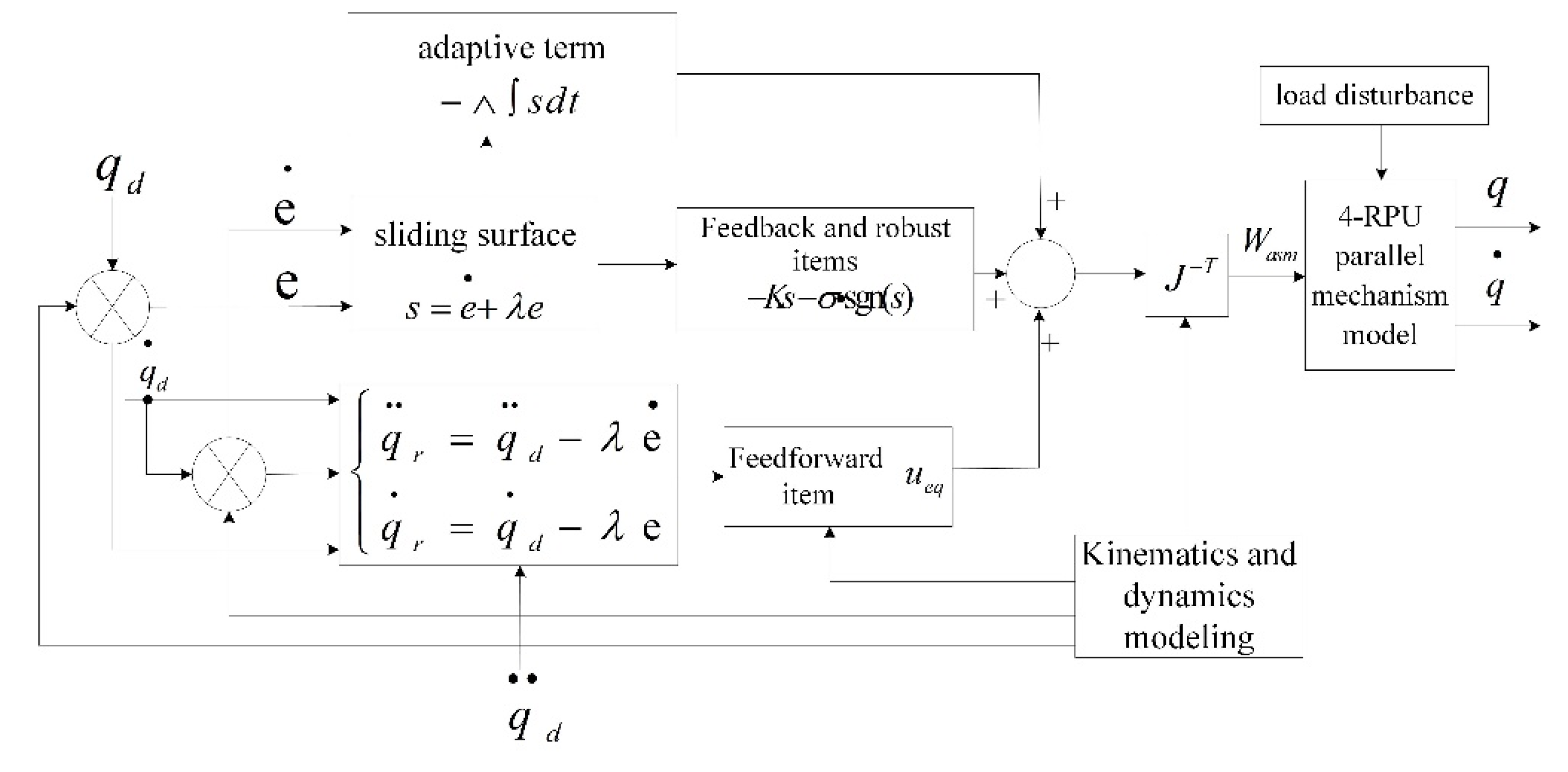
The control block diagram of the adaptive sliding mode system is obtained by Formula (31), as shown in
Figure 6.
5. Control System Simulation Experiment
To verify the effectiveness of the adaptive sliding mode control algorithm, the simulation calculation is programmed in MATLAB-Simulink, and the fourth-order R-K method is used to solve the dynamic response of the mechanism.
5.1. Simulation Parameters
The physical parameters of the mechanism are shown in
Table 1, and the error rate of each parameter is set to 10%. Periodic time-varying loads are applied to the
,
, and
pose directions: 12sin (2t)
, −16cos (1.5t)
, and −25sin (2t)
. The control parameters are:
,
,
,
,
,
, and
.
The pose parameters of the platform are:
To test the convergence performance of the error, it is assumed that there is an initial system error, and the initial state of pose is set as:
The simulation running time is 20 s, and the step length is 0.001 s.
5.2. Analysis of Simulation Results
To evaluate the effect of the control method, an evaluation index is introduced here:
Type: Represents run time; represents the average tracking error.
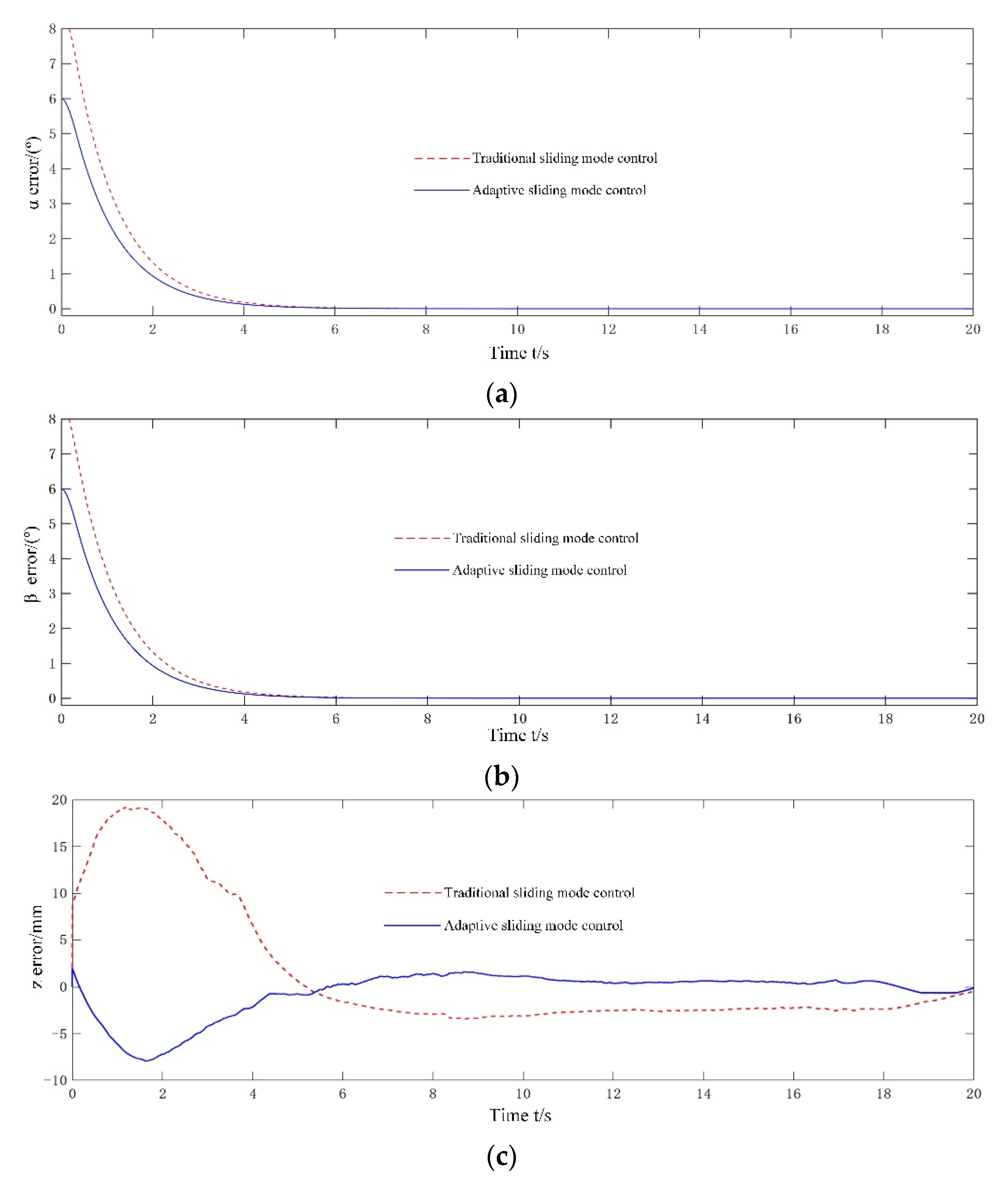
Figure 7 is a comparison of the tracking error curves of each degree of freedom of the moving platform under the traditional sliding mode control (32) and the adaptive sliding mode control (31). As shown in
Figure 7, despite the existence of initial system error and time-varying load disturbance, the tracking error of each degree of freedom can still converge to the equilibrium state within 4 s, which verifies that both control methods can satisfy asymptotic and bounded stability overall.
After reaching a steady-state, the average tracking errors when using the traditional sliding mode control are 0.047°, 0.065°, and 0.551 mm, respectively. In contrast, when the proposed adaptive sliding mode control is used, the corresponding error values are 0.012°, 0.019°, and 0.117 mm, which are reduced by 74.5%, 70.8%, and 78.8%, respectively, and the tracking accuracy is improved. The reason for this is that the adaptive law (34) can effectively estimate the model uncertainty and load disturbance to overcome its influence.
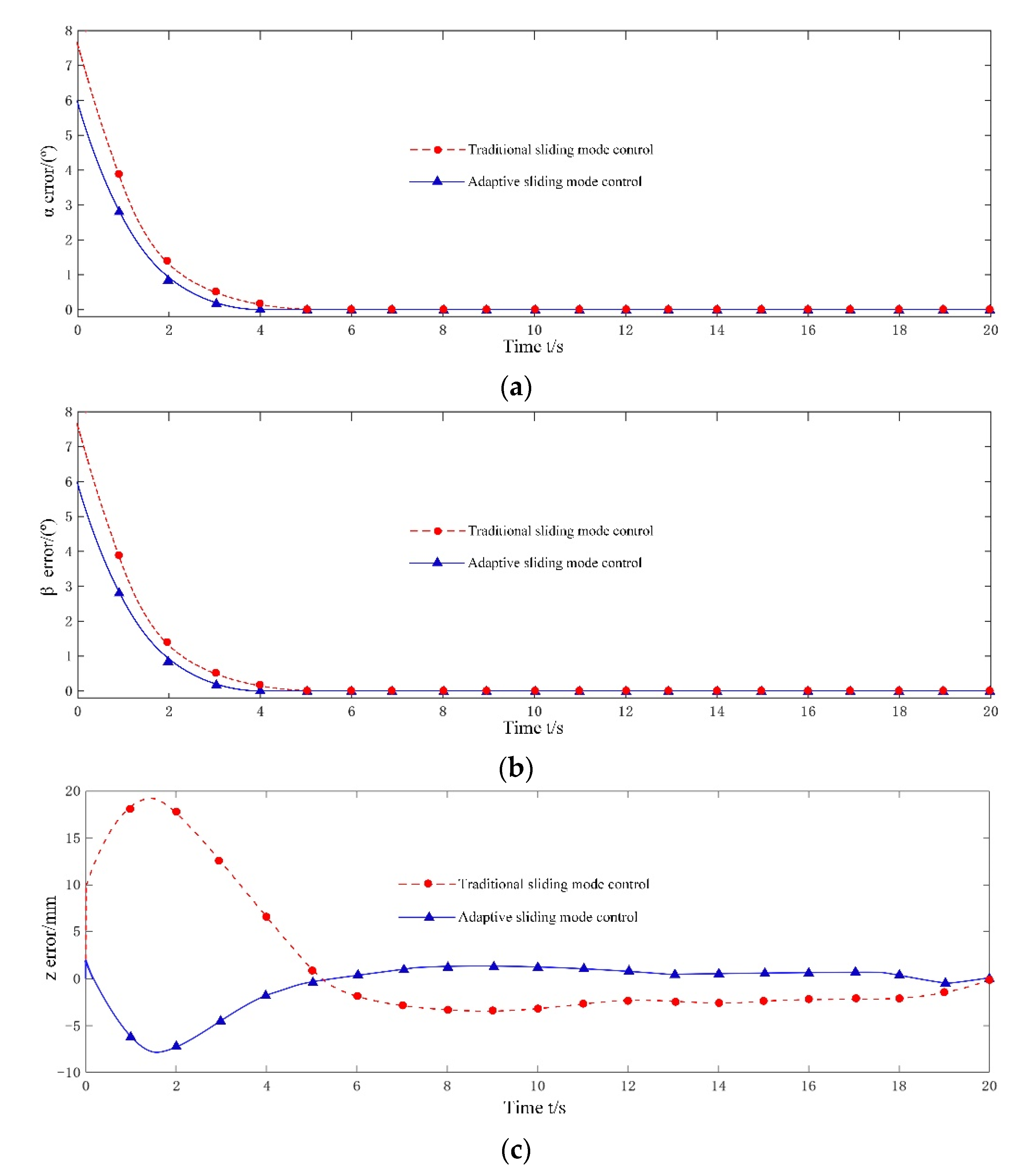
To further verify the reliability of the control method, a joint simulation of MATLAB/Simulink-ADAMS is established. According to the parameters in
Table 1, the three-dimensional model is imported into ADAMS, and the necessary fixed pair, moving pair, and rotating pair are introduced into the model. The driving force/torque in MATLAB is used as the input of ADAMS, whereas the motion parameters in ADAMS are used as the input of MATLAB. The simulation time is set to 20 s, and the results are shown in
Figure 8. According to a comparative analysis of
Figure 7 and
Figure 8, the numerical analysis and simulation results are basically consistent.
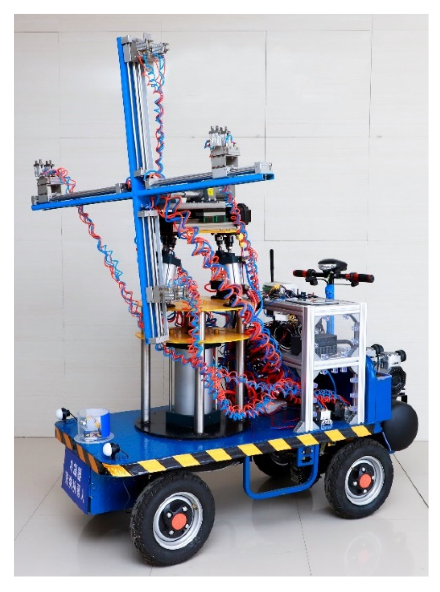
Theoretical calculations and simulation experiments had a certain guiding significance for building the test prototype. The built condenser cleaning robot prototype is shown in
Figure 9.
6. Conclusions
In this study, a hybrid robot for condenser cleaning is designed. According to the mechanism topology calculations, the redundant parallel mechanism has three degrees of freedom, including two rotations and one movement. The kinematics of the 4-RPU mechanism is analysed, laying a foundation for dynamics modelling.
The dynamic model of the 4-RPU redundant parallel mechanism was constructed by using the principle of virtual work. On this basis, the optimisation method of the two-norm solution of the driving force was adopted, and MATLAB was used to solve the driving force of the 4-RPU redundant parallel mechanism. The correctness of the theoretical model was verified by comparison with ADAMS simulation results.
To overcome the uncertainty of the dynamic model of the mechanism, an adaptive sliding mode control with uncertainty estimation capability was proposed. Compared with the active sliding mode control (ASMC) method proposed by Li Long et al., which involves the radial basis function neural network (RBFNN) compensator and Newton–Euler estimator, this method can estimate and compensate parameter uncertainties and load perturbations simultaneously, thus improving the robustness of the system. The simulation results showed that the adaptive sliding mode control could effectively compensate for the time-varying model uncertainty, is insensitive to the change of load disturbance, and has good control performance, a fast response, and high convergence accuracy. Compared with the traditional sliding mode control, the average tracking errors of the moving platform pose are reduced by 74.5%, 70.8%, and 78.8%, respectively, thereby improving the accuracy and efficiency of conventional cleaning robots. We succeeded in building a prototype for the condenser cleaning robot.
Author Contributions
Conceptualization, J.L. and C.W.; methodology, J.L. and C.W.; software, J.L.; validation, J.L. and C.W.; formal analysis, J.L. and C.W.; investigation, J.L.; resources, C.W.; data curation, J.L.; writing—original draft preparation, J.L.; writing—review and editing, J.L. and C.W.; visualization, J.L. and C.W.; supervision, C.W.; project administration, J.L. and C.W. All authors have read and agreed to the published version of the manuscript.
Funding
This research was funded by the 2021 Anhui University Graduate scientific research project of Anhui Provincial Department of Education, grant number YJS20210406.
Institutional Review Board Statement
Not applicable.
Informed Consent Statement
Not applicable.
Data Availability Statement
Not applicable.
Acknowledgments
This work was supported in part by the National Innovation Methods Project, grant number 2018IM010500.
Conflicts of Interest
The authors declare no conflict of interest.
References
- Luo, D.; Dong, B.; Qin, W. Design and control methods of a condenser cleaning robot. Chem. Eng. Trans. 2017, 62, 703–708. [Google Scholar]
- Zhu, X.; Xu, J.; Zhang, L.; Meng, J. Research of thermal and anti-scaling performance of condense tubes with rotor inserts. J. Eng. Thermophys. 2020, 41, 1712–1718. [Google Scholar]
- Ye, W.; Hu, L.; Xia, D.; Zhou, Z. Performance analysis and optimization of redundantly actuated three translational parallel mechanism. Trans. Chin. Soc. Agric. Mach. 2021, 52, 421–430. [Google Scholar]
- Zhang, W.; Xu, L.; Tong, J.; Li, Q. Kinematic analysis and dimensional synthesis of 2-PUR-PSR parallel manipulator. J. Mech. Eng. 2018, 54, 45–53. [Google Scholar] [CrossRef]
- Huang, K.; Shen, H.; Li, J.; Zhu, Z.; Yang, T. Topological design and dynamics modeling of a spatial 2T1R parallel mechanism with partially motion decoupling and symbolic forward kinematics. China Mech. Eng. 2022, 33, 160–169. [Google Scholar]
- Xia, H.; Wang, Y.; Yin, F.; Cao, W. Design and kinematics analysis of large condenser cleaning robot. China Mech. Eng. 2014, 25, 103–107. [Google Scholar]
- Zhao, L.; Yan, Z.; Luan, Q.; Zhao, X.; Li, B. Kinematic calibration and error analysis of 3-RRRU parallel robot in large overall motion. Trans. Chin. Soc. Agric. Mach. 2021, 52, 411–420. [Google Scholar]
- Zhang, J.; Shi, H.; Wang, T.; Huang, Q.; Jiang, L. Analysis of 5-DOF parallel driving mechanisms and their position resolution. China Mech. Eng. 2021, 32, 1414. [Google Scholar]
- Li, Y.; Guo, Y.; Zhang, Y.; Zhang, L. Dynamic modeling method of spatial passive over-constrained parallel mechanism based on newton euler method. J. Mech. Eng. 2020, 56, 48–57. [Google Scholar]
- Li, Y.; Zheng, H.; Sun, P.; Xu, T.; Wang, Z.; Qin, S. Dynamic modeling with joint friction and research on the inertia coupling property of a 5-PSS/UPU parallel manipulator. J. Mech. Eng. 2019, 55, 43–52. [Google Scholar] [CrossRef]
- Hou, Y.; Deng, Y.; Zeng, D. Dynamic modelling and properties analysis of 3RSR parallel mechanism considering spherical joint clearance and wear. J. Cent. South Univ. 2021, 28, 712–727. [Google Scholar] [CrossRef]
- Chen, X.; Sun, D.; Wang, Q. Rigid dynamics modeling of redundant actuation parallel mechanism based on lagrange method. Trans. Chin. Soc. Agric. Mach. 2015, 46, 329–336. [Google Scholar]
- Zhu, W.; Guo, Q.; Ma, Z.; Shen, H.; Wu, G. Stiffness and dynamics analysis of SCARA parallel mechanism. Trans. Chin. Soc. Agric. Mach. 2019, 50, 375–385. [Google Scholar]
- Liu, X.; Tang, Y.; Liu, X.; Li, Q.; Zhao, Y. Dynamics performance optimization for redundantly actuated parallel manipulator with constraint branch. Trans. Chin. Soc. Agric. Mach. 2021, 52, 378–385, 403. [Google Scholar]
- Li, Y.; Wang, L.; Luo, Y.; Sun, P.; Zheng, H. Dynamic modeling and dynamic load distribution optimization of a spherical 5R parallel mechanism. Opt. Precis Eng. 2018, 26, 2012–2020. [Google Scholar]
- Yang, H.; Fang, H.; Fang, Y. Dynamics analysis and simulation of a novel parallel perfusion robot. J. Cent. South Univ. 2019, 50, 2118–2127. [Google Scholar]
- Chai, X.; Yang, Y.; Xu, L.; Li, Q. Dynamic modeling and performance analysis of a 2-UPR-RPU parallel manipulator. J. Mech. Eng. 2020, 56, 110–119. [Google Scholar]
- Lin, G.; Liao, X.; Zhao, R.; Chen, S. Dynamics and power analysis of 2-UPR&2-RPU redundant parallel mechanism. Adv. Eng. Sci. 2021, 53, 146–154. [Google Scholar]
- Zhao, J.; Sun, X.; Dong, J.; Wang, C.; Xu, J.; Wang, Z. Sliding mode decoupling control for electro-hydraulic multidimensional force loading system with parallel mechanism. J. Cent. South Univ. 2020, 51, 3407–3417. [Google Scholar]
- Zhao, J.; Wang, C.; Xu, J.; Dong, J.; Sun, X.; Zhao, Z. CMAC-fuzzy PID control of multi-dimensional force loading system of hydraulic drive parallel mechanism. J. Cent. South Univ. 2021, 51, 2811–2821. [Google Scholar]
- Cui, X.; Chen, W.; Han, X.; Zhu, X.; Wang, J.; Cheng, Q. Active compliant control strategy of 3RPS/UPS parallel machine with redundant actuating leg based on lagrange equation. Comput. Integr. Manuf. Syst. 2016, 22, 2434–2441. [Google Scholar]
- Niu, X.; Gao, G.; Liu, X.; Bao, Z. Dynamics and control of a novel 3-DOF parallel manipulator with actuation redundancy. Int. J. Automat. Comput. 2013, 10, 552–562. [Google Scholar] [CrossRef] [Green Version]
- Navabi, H.; Sadeghnejad, S.; Ramezani, S.; Baltes, J. Position control of the single spherical wheel mobile robot by using the fuzzy sliding mode controller. Adv. Fuzzy Syst. 2017, 2017, 2651976. [Google Scholar] [CrossRef] [Green Version]
- Zhang, B.; Zhang, F.; Zhou, F.; Shang, W.; Cong, S. Dual-space adaptive synchronization control of cable-driven parallel robots. Robot 2020, 42, 139–147. [Google Scholar]
- Liu, S.; Peng, G.; Gao, H. Dynamic modeling and terminal sliding mode control of a 3-DOF redundantly actuated parallel platform. Mechatronics 2019, 60, 26–33. [Google Scholar] [CrossRef]
- Liu, Y.; Wang, X.; Zhao, G.; Ma, S. Position-pose control of a pneumatic 3-upu robot based on immersion and invariance. Int. J. Control. Autom. Syst. 2022, 20, 956–967. [Google Scholar] [CrossRef]
- Li, L.; Wang, C.; Guo, Y.; Wu, H. Research on dynamics of hybrid pouring robot and attitude stability control of ladle. Meas. Control 2020, 53, 564–576. [Google Scholar] [CrossRef] [Green Version]
| Publisher’s Note: MDPI stays neutral with regard to jurisdictional claims in published maps and institutional affiliations. |
© 2022 by the authors. Licensee MDPI, Basel, Switzerland. This article is an open access article distributed under the terms and conditions of the Creative Commons Attribution (CC BY) license (https://creativecommons.org/licenses/by/4.0/).


