PI Speed Control with Reverse Motion of a Series DC Motor Based on the Noise Reduction Disturbance Observer

Abstract

In this paper, the speed control of a series DC motor is presented together with the electronics necessary to ensure inverse motion. The control law is based on the classical PI controller and the noise reduction disturbance observer (NRDOB). This control strategy allows the use of a linear approximation of the motor dynamics due to its excellent properties regarding model uncertainties, sensor noise, and external perturbations. Consequently, a linear model based on the nonlinear modelling with magnetic saturation of the motor is also presented. The NRDOB-based control frequency-domain approach allows for the treating of structured and unstructured disturbances in the spirit of classical control theory. Although PI controllers have proved to provide excellent performance and robustness for the speed control of series DC motor, it cannot cope, without affecting or reducing the performance, with the effects of sensor noise; moreover, to further improve the performance, especially in tracking conditions, it is necessary to design and implement a power driver capable of generating inverse motion. In addition, because NRDOB is in fact an internal model control strategy, a perfect match between process and model is not required. That is, contrary to the common belief that the NRDOB is a 2-DOF, it is in fact a 3-DOF control scheme. Based on these characteristics, it was possible to design and implement a robust high-performance speed control system with reverse motion for the non-linear series DC motor with not well-defined relative degree, together with the electronics required for the reverse motion which is fully described. This results in a control system capable of overcoming the problems generated by input disturbances and sensor noise, ensuring robustness and performance in tracking and regulation conditions. Real-time experimental results are included in support of the approach presented here.

1. Introduction

Series DC motors, as well as series universal motors, are electric motors with one voltage supply and the field winding connected in series with the rotor winding. This series connection results in a motor with very high starting torque. However, the force decreases as the speed increases due to an increment of the back counter electromotive force (EMF). This is why series DC motors have poor speed regulation. That is, increasing the motor load tends to slow its speed, which in turns reduces the back EMF and increases the torque to accommodate the load. Also, this kind of motor moves in the same direction even though the current through the series windings is reversed. Therefore, reverse motion can be generated only if the polarity of the current flowing to the motor is reversed. This requires a driver—normally an H bridge—capable of providing adequate switching characteristics.

The appropriate design of speed control systems for this kind of motor will surely increase its use and application by better exploiting of its great features—high torque, low current consumption, and small dimensions—all desirable characteristics for electric motors employed as actuators. In particular, these features are required by robotics where low weight, small dimensions, and low current consumption with high torque are highly appreciated. Another possible application for these electric motors is their use in electric vehicles [1,2,3], where high torque with low current consumption is required. The former requires accurate models (linear and nonlinear), proper power drivers and good control schemes. The authors define good control schemes not only by their robustness and performance but by their level of complexity which can impede or facilitate its design and implementation. In a previous article [4], a methodology for the identification of series DC motors based on a nonlinear model without magnetic saturation together with a linearization around an equilibrium point was presented. Moreover, in [4] it is shown that linear models in the form of transfer functions are good models in the design of high performance controllers for a large range of operations. Moreover, in [5], the design of the nonlinear generalized predictive controller for series DC motors showed that this kind of motor has a non-well defined relative degree in conditions where the current or the rotor speed is zero, so exact linearization cannot be obtained if reverse motion is required. Due to this characteristic, some early reports and articles published, regarding the design of speed control systems for series DC motor, are devoted to using the series DC motor model as an academic example to analyze, design and assess different control strategies for systems with a non-well defined relative degree [6,7,8], or to assess control approaches—nonlinear, linear, fuzzy logic, fractional—without considering reverse motion [9,10,11,12,13,14,15,16]. Moreover, most of them are limited to validations based on digital simulations. On the other hand, articles reporting real-time implementation focus mainly on the power driver without inverting motor polarization [17,18,19,20,21,22]. The authors are aware of only one attempt to implement a speed control system for a series DC motor, including necessary electronics to generate reverse motion but, regrettably, with unrealistic current consumption of around 150 A [23]. Therefore, this article represents a novel result for the speed control problem of series DC motor.

Although [4] proved that simple PI controllers can provide good performance in regulation and tracking in the speed control of series DC motors, it was also shown that sensor noise unnecessarily increases control efforts. Moreover, it was found that the potential of any controller is highly affected by the impossibility of inverting the magnetic torque or the direction of rotation, especially in tracking conditions. Therefore, it is necessary to solve these problems to improve the speed control system of series DC motors. In this context, the main contributions of this paper are the analysis, design, and implementation of a speed control system with reverse motion for a series DC motor that is easy to design and implement and which also guarantees performance, robustness, and disturbance rejection.

The approach followed here to address these problems is founded on the use of the noise reduction disturbance observer (NRDOB) [24], as a way to reduce the effects of sensor noise, and the design and construction of a power driver based on an “H-bridge” to commute polarization of the motor, such that inverse motion can be achieved. Additionally, a linear approximation around an equilibrium point is presented based on the derivation of a nonlinear model with magnetic saturation of the series DC motor.

The NRDOB, in conjunction with many control strategies, has proved to be an excellent approach to overcome perturbations and noises, especially sensor noise. An important feature of the NRDOB is that, apart from being suitable for many applications, it is a scheme easy to design as it depends only on the design of a low-pass filter with unity steady-state gain [25,26,27,28,29].

Although the first NRDOB articles are from the early 2010s, conditions for their stability have been partially reported. Global conditions for stability and robustness based on the Nyquist stability criteria were reported by the authors in [30]. It includes the analysis for different kinds of mismatch between the process and its model (model uncertainty) and the procedure to design NRDOB-based controllers for processes with unstable poles, non-minimum phase zeros, or time delays. In this context, the article represents a real-time application of an NRDOB control system proving the theoretical results of [30] and the excellent results NRDOB can provide. Moreover, as reported in [31], NRDOB also represents an alternative to reduce problems associated to input/output perturbations in the implementation of recursive identification algorithms. Additionally, NRDOB-based control systems have proved to be suitable for many applications such as robotics, aeronautics, and electric machines [32,33,34].

Although the main objective of this article is to present an integral solution based on the NRDOB approach and the necessary electronics to ensure the reverse movement of the speed control problem with reverse movement of a DC Series motor, the use of the NRDOB is justified by the fact that it provides a simple solution to reduce the effects of input signal disturbances and sensor noise without compromising the stability and performance of the overall control system. In addition, stability, and performance robustness against parametric uncertainty and unmodeled dynamics is also guaranteed according to the results presented in [30] where global stability and robustness conditions based on Nyquist stability criteria were established. Likewise, it was also shown that a perfect or approximate match between the process and the model process is not necessary. Performance is achieved by the fact that a control system based on the NRDOB is an internal model control (IMC) scheme as show above in Equation (33). Contrary to other approaches, the NRDOB was designed to reduce not only input disturbances but also sensor noise effects in a simple way. That is, in the case of a stable minimum phase process such as the series DC motor it only requires the design of a controller capable of stabilizing the model process and the design of a filter with unity steady-state gain. For more details regarding complex processes (unstable, non-minimum phase or with delays) the reader can consult [30].

However, various approaches have been proposed to overcome or reduce the problem of disturbances affecting the control signal (process input signal). Most of them are based on state space analysis. For example, the active disturbance rejection control (ADRC) [35,36,37] consisting of constructing an extended state where the states of the system and the disturbance are grouped to later implement and state observer. Although this approach requires only the knowledge of process relative degree, it does not deal with the sensor noise problem; also, it can be applied only to the stable process or previously stabilized processes. In [38,39], the disturbance accommodation control (DAC) is proposed, consisting of a state observer plus an observer for a suggested exogenous perturbation system. This strategy requires one to know the process degree and, like the DARC, it can be applied only to a stable process or previously stabilized processes. Other approaches, such as disturbance and uncertainty estimation (DUE) [40] and equivalent input disturbance (EID) [41,42] are also based on designing an observer for a proposed exogenous input disturbance system but with an additional filter like the NOB and NRDOB F(s) filter. These approaches require process degree knowledge, in the case of the DUE, and the use of an inverse or pseudo-inverse (for cancellation) in the case of EID. This, of course, reduces its application to minimum phase process. It should be noted that these approaches do not attack the sensor noise problem. In the context of nonlinear systems, several approaches remove input disturbance via a controller in the same way as that applied to achieve exact linearization, that is, by exact cancellation [39]. This requires an accurate process model and a cannot be applied to processes with non-well define relative degree.

The article is organized as follows. In Section 2, a series DC motor nonlinear model with magnetic saturation is presented and in Section 3, the linearization around an equilibrium point of the nonlinear model is derived. In Section 4, a brief presentation of the NRDOB is shown together with a comparison to the internal model control (IMC) and the disturbance observer (DOB). In Section 5, the power driver capable of inverting the polarization of the motor is described. In Section 6, the design of the NRDOB_PI speed control system for the series DC motor and rea- time experimental results are shown. Finally, Conclusions are presented in Section 7.

2. Series DC Motor Nonlinear Model

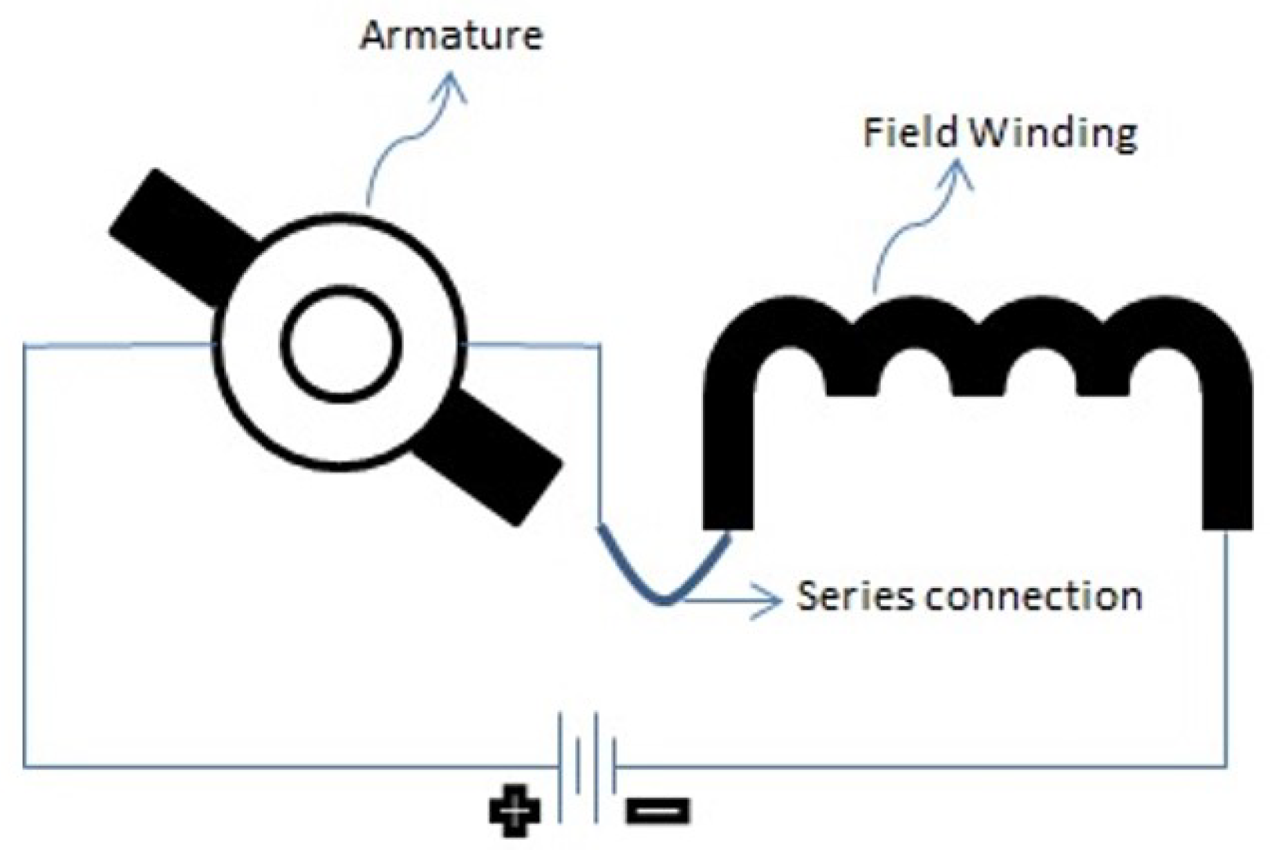
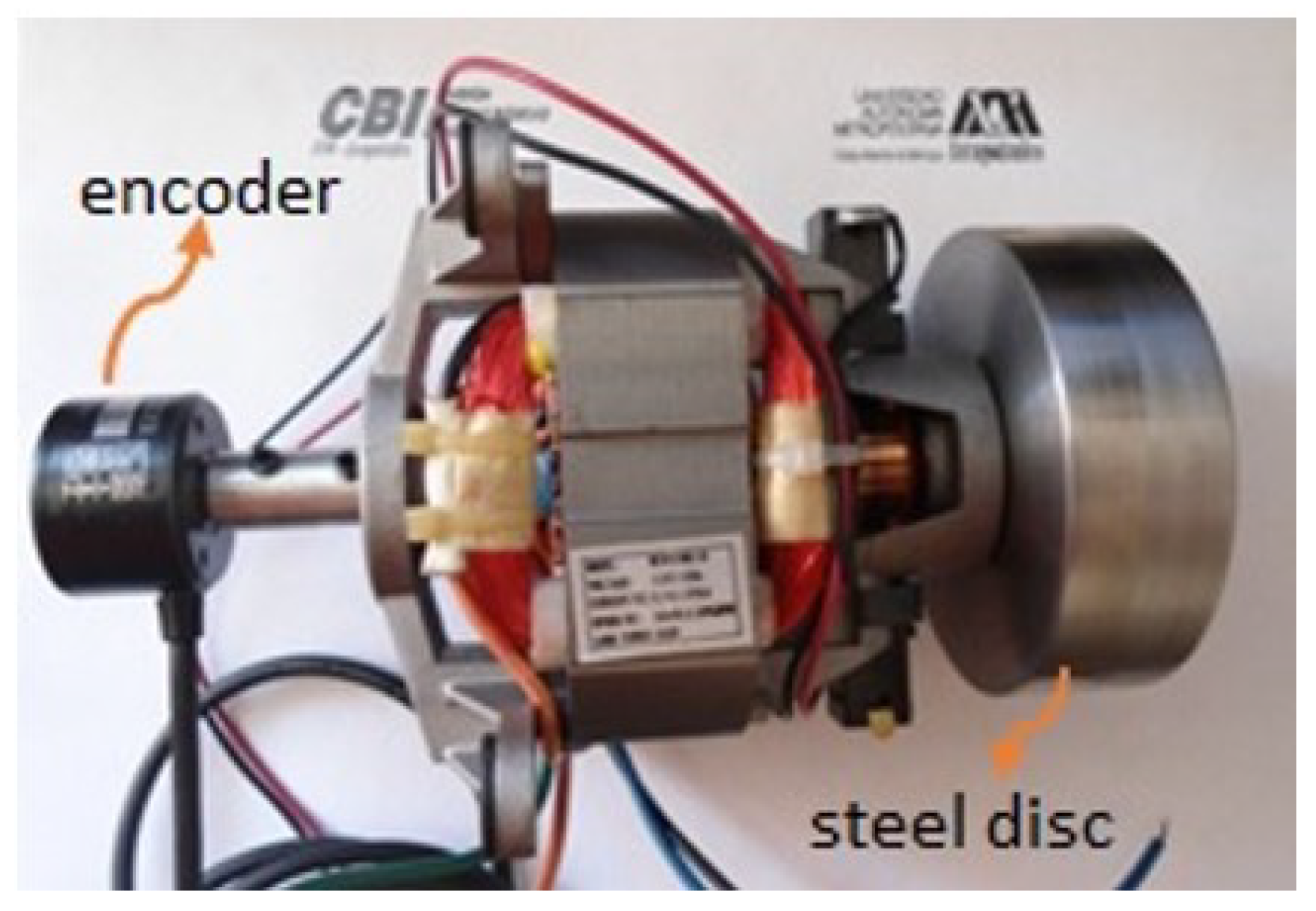
A series-wound DC motor, similar to the shunt wound DC motor or compound wound DC motor, is a self-excited DC motor. It gets this name because the field winding is internally connected in series to the armature winding as shown in Figure 1. They are also considered self-excited motors because instead of two separate voltage sources—one for the armature and one for the field winding—they require only one voltage source.

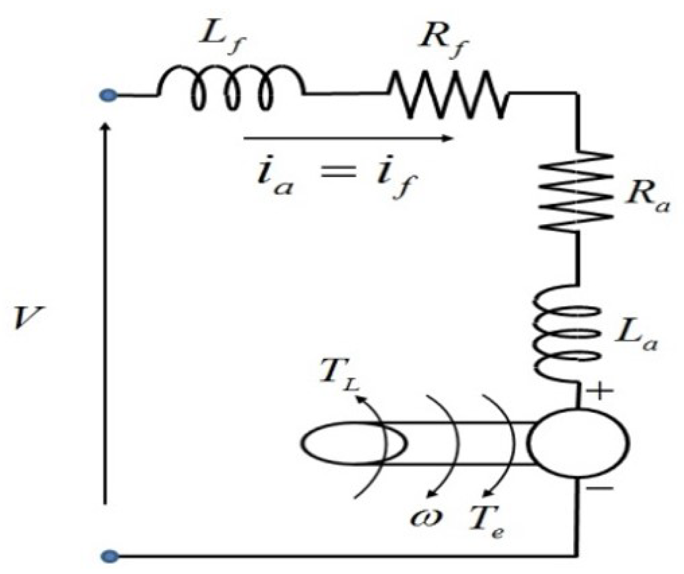
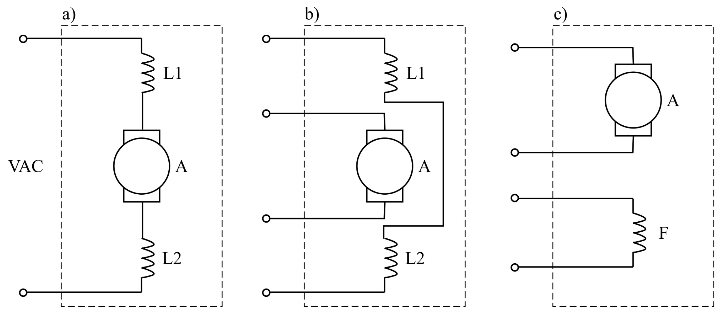
The electric diagram of the series-wound DC motor is shown in Figure 2.

Based on the electric diagram of the series DC motor, the differential equations comprising the electrical and mechanical subsystems of a series DC motor are given by [43]

$$V\left(t\right)=R_a{i}_a\left(t\right)+R_f{i}_f\left(t\right)+L_a\frac{d}{dt}{i}_a\left(t\right)+L_f\frac{d}{dt}{i}_f\left(t\right)+E_a$$

(1)

$$T_e\left(t\right)=T_L\left(t\right)+b\omega \left(t\right)+J\frac{d}{dt}\omega \left(t\right).$$

(2)

Because $i_a\left(t\right)=i_f\left(t\right)$, Equation (1) reduce to

$$V\left(t\right)=\left(R_a+R_f\right)i\left(t\right)+\left(L_a+L_f\right)\frac{d}{dt}i\left(t\right)+E_a\left(t\right)$$

(3)

where, $\omega \left(t\right)$ is the rotor speed, $E_a\left(t\right)$ represents the EMF, $T_L\left(t\right)$ is the load torque, $i\left(t\right)=i_a\left(t\right)=i_f\left(t\right)$ is the current, b is the friction coefficient and $T_e\left(t\right)$ the electromagnetic torque produced by the motor.

The EMF $E_a\left(t\right)$ and $T_e\left(t\right)$ depend both on the air-gap flux $\mathsf{\Phi }$, that is,

$$E_a\left(t\right)=\omega \left(t\right)\mathsf{\Phi }$$

(4)

$$T_e\left(t\right)=i\left(t\right)\mathsf{\Phi }.$$

(5)

The flux $\mathsf{\Phi }\left(i\right)$ is a function of the current $i\left(t\right)$, so Equations (2) and (3) are non-linear. Also, it is common practice to approximate the flux $\mathsf{\Phi }\left(i\right)$ by a linear relationship when magnetic saturation is neglected, that is

$$\mathsf{\Phi }\left(i\right)=k_{0}i\left(t\right)$$

(6)

where, $k_0$ is the mutual inductance between the armature and field coils.

Nonetheless, a more realistic model, including magnetic saturation, can be obtained by replacing $k_0$ by a function $K\left(i\right)$

$$\mathsf{\Phi }\left(i\right)=K\left(i\right)i\left(t\right).$$

(7)

It was proved in [44] that $K\left(i\right)$ can be approximated by the rational function

$$K\left(i\right)=\frac{k_0}{\left(1+\overline{b}i\right)}$$

(8)

where, $\overline{b}$ is a positive constant in the range of 0.025–0.035 A${}^{-1}$.

Based on the rational approximation of $K\left(i\right)$, the differential equations of the series DC motor including magnetic saturation result in

$$V\left(t\right)=\left(R_a+R_f\right)i\left(t\right)+\left(L_a+L_f\right)\frac{d}{dt}i\left(t\right)+\omega \left(t\right)i\left(t\right)\frac{k_0}{\left(1+\overline{b}i\left(t\right)\right)}$$

(9)

$$i^2\left(t\right)\frac{k_0}{\left(1+\overline{b}i\left(t\right)\right)}=T_L\left(t\right)+b\omega \left(t\right)+J\frac{d}{dt}\omega \left(t\right).$$

(10)

3. Model Linearization

It was proved in [5] that the series DC nonlinear model does not have a well-defined relative degree when the current $i\left(t\right)=0$ or the rotor speed $\omega \left(t\right)=0$. Therefore, it cannot be fully linearized by state feedback. However, it is possible to design linear controllers based on a linearization around an equilibrium point of the non-linear model of Equations (9) and (10) [4].

Rearranging Equations (2) and (3), we get

$$\frac{d}{dt}i\left(t\right)=-\frac{R}{L}i\left(t\right)-\omega \left(t\right)i\left(t\right)\frac{k_0}{L\left(1+\overline{b}i\left(t\right)\right)}+\frac{1}{L}V\left(t\right)$$

(11)

$$\frac{d}{dt}\omega \left(t\right)=-\frac{b}{J}\omega \left(t\right)-\frac{1}{J}{T}_L\left(t\right)+i^2\left(t\right)\frac{k_0}{J\left(1+\overline{b}i\left(t\right)\right)}$$

(12)

where $R=R_a+R_f$ and $L=L_a+L_f$, and defining

$$\begin{array}{c}{a}_1=:\frac{b}{J};b_1=:\frac{R}{L}\hfill \\ a_2=:\frac{1}{J};b_2=:\frac{k_0}{L}\mathrm{and}\begin{array}{c}{x}_1=:\omega \\ x_2=:i\end{array},\hfill \\ a_3=:\frac{k_0}{J};b_3=:\frac{1}{L}\hfill \end{array}$$

(13)

the non-linear state space model of a series DC motor with magnetic saturation is given by

$$\begin{array}{c}{\dot{x}}_1=-a_1{x}_1-a_2{T}_L+a_3\frac{x_2^2}{\left(1+\stackrel{\_}{b}{x}_2\right)}\hfill \\ {\dot{x}}_2=-b_1{x}_2-b_2\frac{x_1{x}_2}{\left(1+\stackrel{\_}{b}{x}_2\right)}+b_{3}V\hfill \end{array}$$

(14)

$$\dot{x}=\left[\begin{array}{c}{\dot{x}}_1\\ {\dot{x}}_2\end{array}\right]=\left[\begin{array}{c}-a_1{x}_1-a_2{T}_L+a_3\frac{x_2^2}{\left(1+\stackrel{\_}{b}{x}_2\right)}\\ -b_1{x}_2-b_2\frac{x_1{x}_2}{\left(1+\stackrel{\_}{b}{x}_2\right)}+b_{3}V\end{array}\right]=f(x,u).$$

(15)

The equilibrium point $\left(x_{{}_1}^0,x_{{}_2}^0\right)$ of Equation (7) is given by the positive root for $x_{{}_2}^0$ of

$${\left(x_2^0\right)}^2-\frac{\stackrel{\_}{b}}{a_3}\left(a_1{x}_{{}_1}^0+a_2{T}_L\right)x_{{}_2}^0-\frac{1}{a_3}\left(a_1{x}_{{}_1}^0+a_2{T}_L\right)=0$$

(16)

and

$$V=\frac{b_1}{b_3}{x}_{{}_2}^0+\frac{b_2}{b_3}·\frac{x_{{}_1}^0{x}_{{}_2}^0}{\left(1+\stackrel{\_}{b}{x}_{{}_2}^0\right)}.$$

(17)

The linear approximation of Equation (14) around the equilibrium point of Equation (16) is given by [39]

$$\dot{x}=Ax+Bu;y=Cx$$

(18)

where

$$\begin{array}{c}A={\left.\frac{\delta f(x,u)}{\delta x}\right|}_{x_{{}_1}^0,x_{{}_2}^0}=\left[\begin{array}{cc}-a_1& a_3{x}_{{}_2}^0\left(\frac{2+3\stackrel{\_}{b}{x}_{{}_2}^0}{{\left(1+\stackrel{\_}{b}{x}_{{}_2}^0\right)}^2}\right)\\ -\frac{b_2{x}_{{}_2}^0}{{\left(1+\stackrel{\_}{b}{x}_{{}_2}^0\right)}^2}& -b_1-b_2{x}_{{}_1}^0\left(\frac{1+2\stackrel{\_}{b}{x}_{{}_2}^0}{{\left(1+\stackrel{\_}{b}{x}_{{}_2}^0\right)}^2}\right)\end{array}\right];\hfill \\ \\ B={\left.\frac{\delta f(x,u)}{\delta u}\right|}_{x_{{}_1}^0,x_{{}_2}^0}=\left[\begin{array}{cc}-a_2& 0\\ 0& b_3\end{array}\right];C=\left[\begin{array}{cc}1& 0\end{array}\right]\hfill \end{array}$$

(19)

with

$$u={\left[\begin{array}{cc}{T}_L\left(t\right)& V\left(t\right)\end{array}\right]}^T;y=\omega \left(t\right).$$

(20)

If the load torque $T_L\left(t\right)$ is assumed to be an unknown perturbation, the system becomes a process with one input, voltage $V\left(t\right)$, rendering the modification of the equilibrium point $x_2^0$ and vector B as

$$\begin{array}{c}{x}_{{}_2}^0=\frac{1}{2}\left(\frac{a_1}{a_3}\stackrel{\_}{b}{x}_{{}_1}^0+\sqrt{{\left(\frac{a_1}{a_3}\stackrel{\_}{b}{x}_{{}_1}^0\right)}^2+4\frac{a_1}{a_3}{x}_{{}_1}^0}\right)\hfill \\ B=\left[\begin{array}{c}0\\ b_3\end{array}\right].\hfill \end{array}$$

(21)

From Equations (18)–(21), the transfer function $G\left(s\right)=\frac{\omega \left(s\right)}{V\left(s\right)}=C{\left(sI-A\right)}^{-1}B$, based on the estimated parameters,

Table 1. Motor parameters.

Parameter	Value
$k_0$	0.186 N·m/Wb·A
R	27.75 $\mathsf{\Omega }$
J	0.000666 kg-m${}^2$
b	0.000026 N·m/Wb·A
L	28.011 mH
$x_1^0$	341 rad/s
$\overline{b}$	0.035 A${}^{-1}$

, of the series DC motor reported in [4], results in

$$\frac{\omega \left(s\right)}{V\left(s\right)}=G\left(s\right)=\frac{4353}{s^2+3255s+301.8}.$$

(22)

The poles of the transfer function (22) are $\{-0.092,-3254.82\}$ so the series DC motor results, as expected, in a stable and overdamped process. Moreover, it is possible to differentiate from the poles, two characteristic modes of a DC motor: $\{s+0.092\}$, representing the mechanical subsystem slow dynamic, whereas $\{s+3254.82\}$ represents the fast dynamic of the electrical subsystem.

Although the transfer function (22) was calculated, including the magnetic saturation approximation (8) it has no significant difference with respect to the model without magnetic saturation reported in [4]. This means that both models were obtained in a condition of operation or equilibrium point away from magnetic saturation. Nonetheless, Equations (2) and (3) and the linearization (18)–(21) may represent a better model in those cases in which the motor is operated near magnetic saturation.

4. Noise Reduction Disturbance Observer

The NRDOB is an improvement of the classical DOB that in turn is an improvement of the IMC. The main objective of the IMC is to provide a procedure for the design of feedback controllers, accommodating in a single parameter tuning the design of a control system satisfying performance, robustness, and output disturbance rejection. Due to this property, it is claimed that IMC allows a much simpler procedure than classical control techniques. This, of course, can be widely debated by those who are involved in the design of classical frequency domain controllers based on the graphical indicators Nyquist, Bode, and Nichols chart.

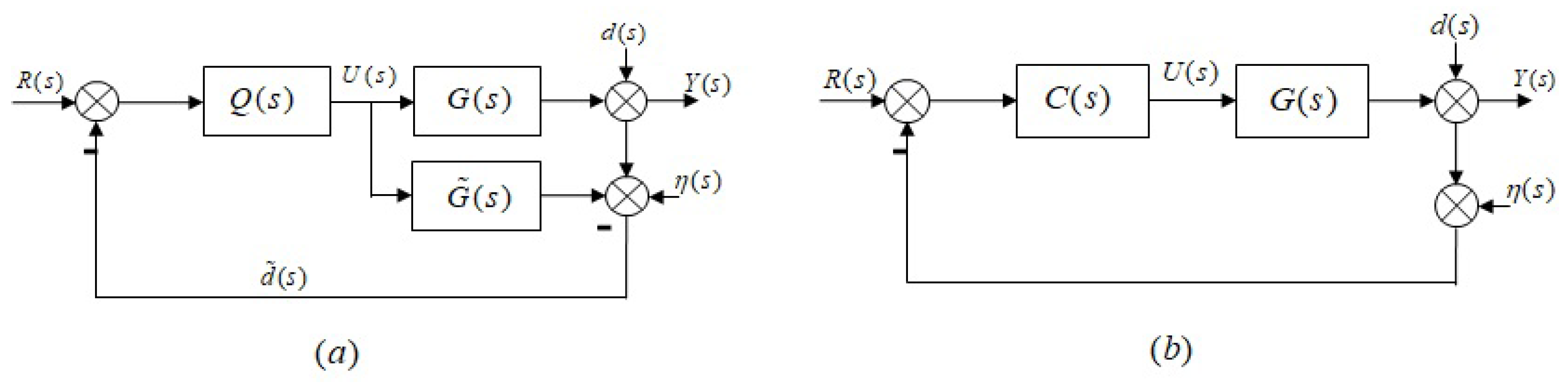
The basic scheme of the IMC is depicted in Figure 3 together with the classical control scheme, where $G\left(s\right)$ is the process, $\tilde{G}\left(s\right)$ the process model, $Q\left(s\right)$ the controller, $R\left(s\right)$ the reference signal and, $d\left(s\right)$ and $\eta \left(s\right)$ the output perturbation and measurement noise signals, respectively. An important fact is that under this scheme, $\tilde{d}\left(s\right)$ is an estimated effect of the perturbation and noise.

In general, controller $Q\left(s\right)$ is based on the cancellation of the stable and minimum phase poles and zeros of $\tilde{G}\left(s\right)$ plus a low pass filter $F\left(s\right)$ necessary to assure causality in $Q\left(s\right)$ as shown in Equation (23)

$$Q\left(s\right)=\tilde{G}{\left(s\right)}^{-1}F\left(s\right)$$

(23)

where $\tilde{G}\left(s\right)$ is a factorization of $G\left(s\right)$ involving only stable poles and minimum-phase zeros of $G\left(s\right)$ and $F\left(s\right)$ is a low pass filter given by

$$F\left(s\right)=\frac{1}{{\left(\lambda s+1\right)}^n}$$

(24)

where n is chosen such that $Q\left(s\right)$ is causal and $\lambda >0$, the constant time of $F\left(s\right)$, is tuned to determine the speed of response. That is, increasing $\lambda$ increases the constant time of the closed loop system, slowing the speed response; on the contrary, reducing $\lambda$ increases the speed response. Also, $\lambda$ must be adjusted to compensate the mismatch or uncertainties between the plant $G\left(s\right)$ and the model $\tilde{G}\left(s\right)$.

From Equation (24), $F\left(s\right)$ satisfies

$$\begin{array}{c}\left|F\left(j\omega \right)\right|\approx 1,\omega \in \left[0,{\omega }_{B_F}\right]\hfill \\ \left|F\left(j\omega \right)\right|\approx 0,\omega \in \left[{\omega }_{B_F}+{\mathsf{\Delta }}_{\omega },\infty \right)\hfill \end{array}.$$

(25)

It is possible to implement the classical control scheme of Figure 3b based on the IMC controller $Q\left(s\right)$ if controller $C\left(s\right)$ is given by

$$C\left(s\right)=\frac{Q\left(s\right)}{1-\tilde{G}\left(s\right)Q\left(s\right)}.$$

(26)

From Figure 3 output $Y\left(s\right)$ for the IMC scheme is given by

$$Y\left(s\right)=\frac{GQ}{1+Q(G-\tilde{G})}R\left(s\right)+\frac{1-\tilde{G}Q}{1+Q(G-\tilde{G})}d\left(s\right)-\frac{GQ}{1+Q(G-\tilde{G})}\eta \left(s\right).$$

(27)

Assuming a perfect match between the process $G\left(s\right)$ and model $\tilde{G}\left(s\right)$, together with Equation (23), Equation (27) becomes

$$Y\left(s\right)=F\left(s\right)R\left(s\right)+\left(1-F\left(s\right)\right)d\left(s\right)-F\left(s\right)\eta \left(s\right).$$

(28)

That is, the IMC offers no advantages over the classical control scheme regarding reduction or suppression of measure noise $\eta \left(s\right)$.

For stability, the IMC control system will be internally stable if and only if $G\left(s\right)$ and $Q\left(s\right)$ are stable or equivalently, the classical control scheme will be internally stable if and only if controller $C\left(s\right)$ decomposed as [45],

$$Q\left(s\right)=\frac{C\left(s\right)}{1+\tilde{G}\left(s\right)C\left(s\right)}$$

(29)

results in controller $Q\left(s\right)$ stable.

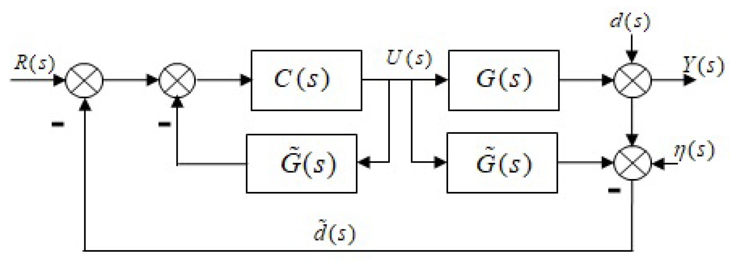
The structure of the IMC evolved to the scheme depicted in Figure 4, which is structurally equivalent to the original IMC but with a more transparent relationship with classical controller $C\left(s\right)$.

An immediate consequence of the IMC controller is the DOB described in Figure 5, where $\delta \left(s\right)$, $\eta \left(s\right)$ and are the input perturbation, output perturbation, and measurement noise, respectively; $C\left(s\right)$, $G\left(s\right)$, $\tilde{G}\left(s\right)$, and $F\left(s\right)$ are the feedback controller, process, process model and a low-pass filter, respectively. The DOB is a control scheme designed to compensate plant uncertainty and output perturbation reduction in conjunction with a feedback controller. Comparing the evolved scheme of the IMC of Figure 4 with the DOB scheme, it is clear that the DOB exploits the same idea of the IMC of plant cancellation plus a low-pass filter separating the disturbance reduction––by means of its observation—from the control action. In Figure 5, the shadowed block represents the DOB. Like IMC, the low-pass filter $F\left(s\right)$ and the inverse of the plant model $\tilde{G}{\left(s\right)}^{-1}$ are defined as in Equations (15) and (16).

From Figure 5, the output $Y\left(s\right)$ is given by

$$Y\left(s\right)=T_R\left(s\right)R\left(s\right)+S_d\left(s\right)d\left(s\right)+S_{\eta }\left(s\right)\eta \left(s\right)+S_{\delta }\left(s\right)\delta \left(s\right)$$

(30)

where

$$\begin{array}{c}{T}_R=\frac{CG\tilde{G}}{Den},S_d=\frac{\tilde{G}\left(1-F\right)}{Den},S_{\delta }=\frac{G\tilde{G}\left(1-F\right)}{Den},S_{\eta }=\frac{G\left(F+C\tilde{G}\right)}{Den}\hfill \\ \\ Den=\tilde{G}\left(1+CG\right)+F\left(G-\tilde{G}\right)\hfill \end{array}.$$

(31)

Assuming that all the roots of the polynomial $Den\left(s\right)$ of Equation (23) are Hurwitz and the low-pass filter $F\left(s\right)$ with a bandwidth ${\omega }_{B_F}$, as indicated in Equation (17), it is clear that in the low range of frequencies $\omega \in \left[0,{\omega }_{B_F}\right]$:

$$\left|T_R\left(j\omega \right)\right|\approx \left|\frac{C\tilde{G}}{1+C\tilde{G}}\left(j\omega \right)\right|,\left|S_d\left(j\omega \right)\right|\approx 0,\left|S_{\delta }\left(j\omega \right)\right|\approx 0,\left|S_{\eta }\left(j\omega \right)\right|\approx 1.$$

(32)

Moreover, if $C\left(s\right)$ is a high-performance feedback controller, Equation (32) reduces to

$$\left|T_R\left(j\omega \right)\right|\approx 1,\left|S_d\left(j\omega \right)\right|\approx 0,\left|S_{\delta }\left(j\omega \right)\right|\approx 0,\left|S_{\eta }\left(j\omega \right)\right|\approx 1.$$

(33)

That is, in the low frequency range, the DOB ensures good signal reference tracking, input and output perturbation reduction but not measurement noise reduction.

On the other hand, in the high-frequency range $\omega \in \left[{\omega }_{B_F}+\mathsf{\Delta },\infty \right)$, where normally $r\left(\omega j\right)=d\left(\omega j\right)=\delta \left(\omega j\right)\approx 0$, $S_{\eta }$ approximates to

$$\left|S_{\eta }\left(j\omega \right)\right|\approx \left|\frac{CG}{1+CG}\left(j\omega \right)\right|.$$

(34)

That is, the DOB offers no advantages over the classical controller or IMC controller regarding measure noise suppression. In other words, improving performance, input and output disturbance rejection, and uncertainty compensation acts in opposition to measured noise reduction and vice versa.

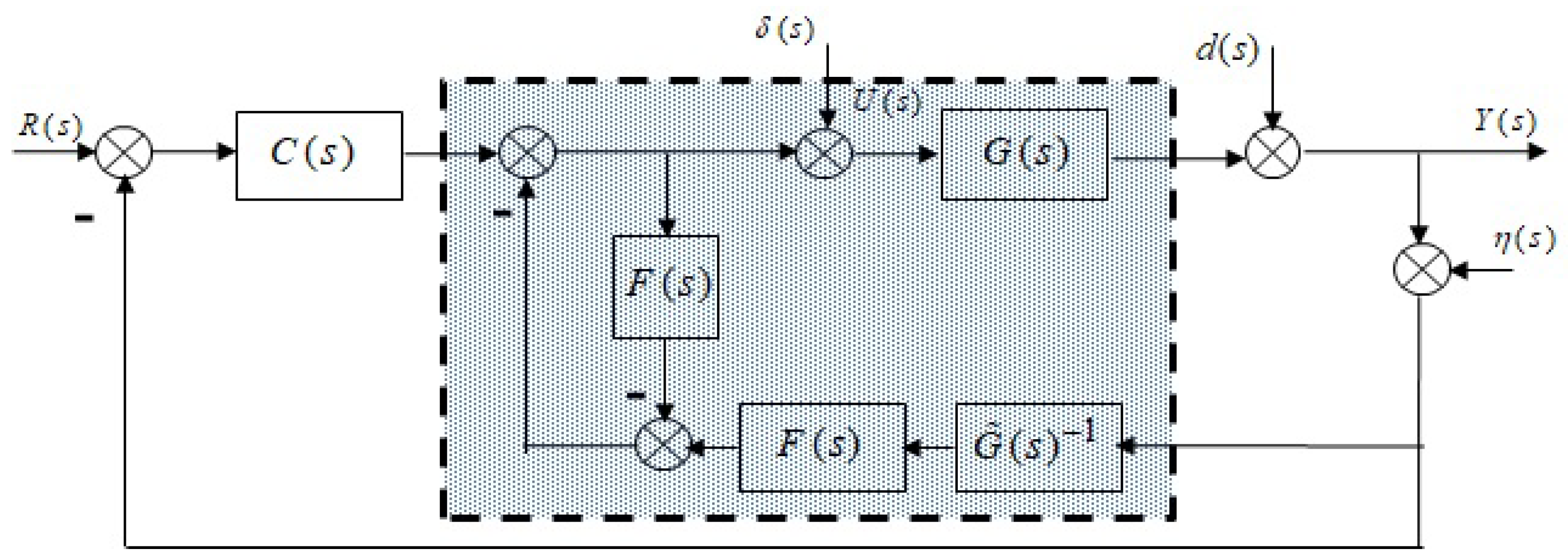
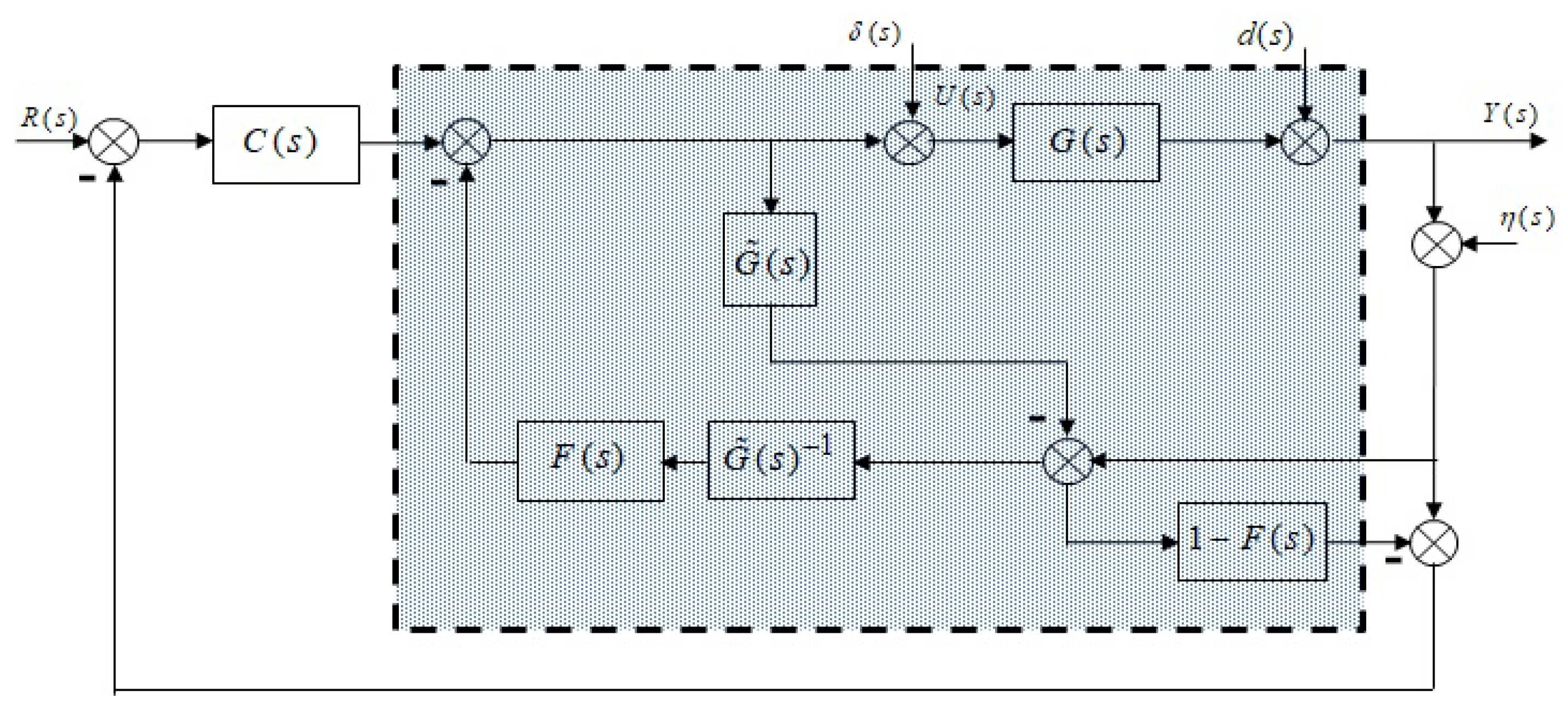
In order to overcome this problem, the NRDOB was proposed [30,46]. The NRDOB has all advantages of the original DOB but with the possibility of reducing the effects of measured noise. In Figure 6, the shadowed block shows the NRDOB scheme where $\delta \left(s\right)$, $d\left(s\right)$, $\eta \left(s\right)$, $C\left(s\right)$, $G\left(s\right)$, $\tilde{G}\left(s\right)$ and $F\left(s\right)$ are defined in same way as for the DOB. It is also assumed that, at low frequency, $\left|\eta \left(j\omega \right)\right|\approx 0$; whereas, at high frequency, $\left|\eta \left(j\omega \right)\right|\ne 0$. This is a normal condition when $\eta \left(s\right)$ represents sensor noise.

Similar to the DOB scheme, output $Y\left(s\right)$ is given by

$$Y\left(s\right)=T_R\left(s\right)R\left(s\right)+S_d\left(s\right)d\left(s\right)+S_{\delta }\left(s\right)\delta \left(s\right)+S_{\eta }\left(s\right)\eta \left(s\right)$$

(35)

where

$$\begin{array}{c}{T}_R=\frac{CG\tilde{G}}{\left(1+\tilde{G}C\right)\left[\tilde{G}+F\left(G-\tilde{G}\right)\right]};S_d=\frac{\tilde{G}\left(1-F\right)}{\tilde{G}+F\left(G-\tilde{G}\right)}\hfill \\ S_{\delta }=\frac{G\tilde{G}\left(1-F\right)}{\tilde{G}+F\left(G-\tilde{G}\right)};S_{\eta }=\frac{GF}{\tilde{G}+F\left(G-\tilde{G}\right)}.\hfill \end{array}$$

(36)

Assuming all the roots of the polynomial $\left(1+\tilde{G}C\right)\left[\tilde{G}+F\left(G-\tilde{G}\right)\right]=0$ of Equation (36) Hurwitz, at low frequency $\omega \in \left[0,{\omega }_{B_F}\right]$, where $\left|F\left(j\omega \right)\right|\approx 1$, the NRDOB reduces to the DOB. That is, at low frequency the NRDOB behaves exactly as the DOB. On the other hand, at high frequency $\omega \in \left[{\omega }_{B_F}+{\mathsf{\Delta }}_{\omega },\infty \right)$$\left|F\left(j\omega \right)\right|\approx 0$, Equation (36) becomes:

$$\left|T_R\left(j\omega \right)\right|\approx \left|\frac{CG}{1+C\tilde{G}}\left(j\omega \right)\right|,\left|S_d\left(j\omega \right)\right|\approx 1,\left|S_{\delta }\left(j\omega \right)\right|\approx \left|G\left(j\omega \right)\right|,\left|S_{\eta }\left(j\omega \right)\right|\approx \left|\frac{G}{\tilde{G}}F\left(j\omega \right)\right|.$$

(37)

Comparing Equation (37) with Equation (34), in contrast to the DOB, with a suitable filter design $F\left(s\right)$, the effects of the measurement noise $\eta \left(s\right)$ can be reduced without compromising the tracking performance of reference signal $R\left(s\right)$. Although input and output perturbations seem to have undesired effects $\left|S_d\left(j\omega \right)\right|\approx 1$, $\left|S_{\delta }\left(j\omega \right)\right|\approx \left|G\left(j\omega \right)\right|$ at high frequency, as mentioned above, these perturbations are assumed negligible above ${\omega }_{B_F}$; that is, $d\left(j\omega \right)=\delta \left(j\omega \right)\approx 0$ when $\omega >{\omega }_{B_F}$. Therefore, the NRDOB is an excellent control strategy option to reduce the effects of measurement noise without compromising the performance of the control system.

Regarding robustness and stability for the NRDOB, in [30], based on the Nyquist stability criteria, global stability conditions for robustness and stability were established together with procedures to the analysis and design of NRDOB control systems assuming or considering different kinds of mismatches between process models $\tilde{G}\left(s\right)$ and processes $G\left(s\right)$. Conditions for stability and robustness are given by the following two Lemmas.

Lemma 1.

The NRDOB control system of Figure 6 will be globally and internally stable if:

(i)

Polynomial $A\left(s\right)=\left(1+\tilde{G}\left(s\right)C\left(s\right)\right)=0$ is stable; that is, controller $C\left(s\right)$ must stabilize plant model $\tilde{G}\left(s\right)$.

(ii)

Polynomial $B\left(s\right)=\left[\tilde{G}+F\left(G-\tilde{G}\right)\right]=\left[1+F\left(s\right)\left(\frac{G\left(s\right)}{\tilde{G}\left(s\right)}-1\right)\right]=\left[1+F\left(s\right)H\left(s\right)\right]=0$ is stable; that is, $F\left(s\right)$ must stabilize $H\left(s\right)=\left(\frac{G\left(s\right)}{\tilde{G}\left(s\right)}-1\right)=-\left(1-\frac{G\left(s\right)}{\tilde{G}\left(s\right)}\right)=\frac{G\left(s\right)-\tilde{G}\left(s\right)}{\tilde{G}\left(s\right)}$.

Lemma 2.

The NRDOB control system of Figure 6 will be robust if:

(i)

$C\left(j\omega \right)$ must be designed such that $C\left(j\omega \right)\tilde{G}\left(j\omega \right)$ have adequate gain and phase margins

(ii)

$F\left(j\omega \right)$ is designed such that $F\left(j\omega \right)H\left(j\omega \right)$ have adequate gain and phase margins.

5. Power Driver

It is necessary to design and implement a power driver capable of inverting the polarity of connection of the voltage supply to the motor to allow the possibility of reverse motion in a series DC motor. This requires electronics with safety circuitry, in addition to the implementation of sensors (current and rotor position) and data acquisition electronics are required to achieve real-time monitoring and control. The design of the power driver was based on the monophasic universal motor from the Koblenz model HC8825M110 with a couple loads of a steel disc of 0.920 kg, nominal maximum speed and power of 24,000 RPM and 0.815 HP, respectively. Current consumption of 0.88 A in steady-state and up to 3.3 A at start up. Also, for sensing the position, speed, and direction of the rotation of the rotor, an incremental encoder of 1024 ppr was installed (see Figure 7).

This type of motor is assembled with a field coil, split into $L_1$ and $L_2$, connected in series with the armature coils A, as shown in Figure 8a. To be able to invert the direction of rotation of the rotor it is necessary that the current in the armature always circulates in the same direction while, at the same time, the sense of the field current can be reversed. To achieve this, it was necessary to separate coils $L_1$ and $L_2$ from the armature coil A to later join them into a single coil F (Figure 8b,c). With this reconnection it is possible to feed the field and armature coils independently.

The general scheme of electronic circuits that allows, in a controlled and safe way, reversing the polarization of the motor field coil is shown in Figure 9. The designed electronic circuits allow for the reversal of the direction of rotation of the rotor and monitoring rotor speed, position, and current consumption. In order to operate the motor in real time, it is also necessary a conditioning and signal processing stage.

5.1. Power Electronics Stage

The most important block is the power electronics stage (Figure 9, Block 1) which provides the necessary energy to operate and invert the direction of motion of the motor according to the controller requirements. This circuitry is able to withstand reverse currents when the motor slows down or when the controller demands a change in the direction of rotation. To achieve reverse direction of rotation, it is necessary to reverse the magnetic flux of the field winding. This is done by connecting the field coil in an “H-Bridge” build with the integrated circuit LMD18200 which includes 4 MOSFET transistors [47,48]. The transistor commutation reverses the current direction passing by the field with respect to the armature with which the magnetic flux and the direction of rotation are also reversed. The maximum operating voltage of the power stage is 50 VDC which are supplied by a laboratory voltage source. In Figure 10 the schematic diagram of the power stage is shown.

5.2. Protection Circuit

The main purpose of the protection circuit (Figure 9, Block 2) is to maintain the feeding voltage below the maximum voltage of operation 55 VDC of the LMD18200. The protection circuit is able to resist inverse connections; that is, if the motor power supply is mistakenly connected in reverse. The schematic diagram of the protection circuit is shown in Figure 11.

5.3. Data Acquisition Stage

The data acquisition stage is the interface between the PC and the power stage (Figure 9, block 3). It receives from the PC the value of the rotor speed by a PWM signal in order to activate the power stage. It also takes the current consumption value and the encoder signals as shown in the interface schematic diagram of Figure 12.

5.4. Power Supplies

This circuit provides voltage sources to all power driver stages (Figure 9, block 4) It consists of 3 linear sources providing: VCC = +5 V @ 1 A, VDD = +12 V @ 0.5 A and VSS = −12 V @ 0.5 A. It includes a protection stage against peak voltages as shown in Figure 13.

6. Control System Design

The design of the control system is based on the simplification of the motor model of Equation (14) by applying pole dominance. That is, from its poles $\{-0.092,-3254.82\}$, pole $s=-3254.82$ can be neglected.

Based on this simplification the linear model of the series DC motor results in

$$\tilde{G}\left(s\right)=\frac{14.423459}{\left(10.78498s+1\right)}.$$

(38)

The model simplification is also justified by the conditions of design defined as

• Bandwidth ${\omega }_B$ in the range of 1 to 2 rad/s;
• Phase margin $M_p>80$° and Gain margin $M_g\to \infty$;
• Steady state error $e_{ss}\to 0$ in regulation conditions;

These conditions were set in order to avoid saturation in the input voltage control signal with a time response of around of 2 to 4 s. However, saturation must be expected if reference signal $R\left(s\right)$ Figure 6 has sudden changes like those presented when $R\left(s\right)$ is defined by a train of square pulses. Based on these design specifications and conditions $\left(i\right)$ of Lemmas 1 and 2, an appropriate feedback controller $C\left(s\right)$ is given, the PI controller is given by

$$C\left(s\right)=\frac{\left(1.122s+0.104\right)}{s}.$$

(39)

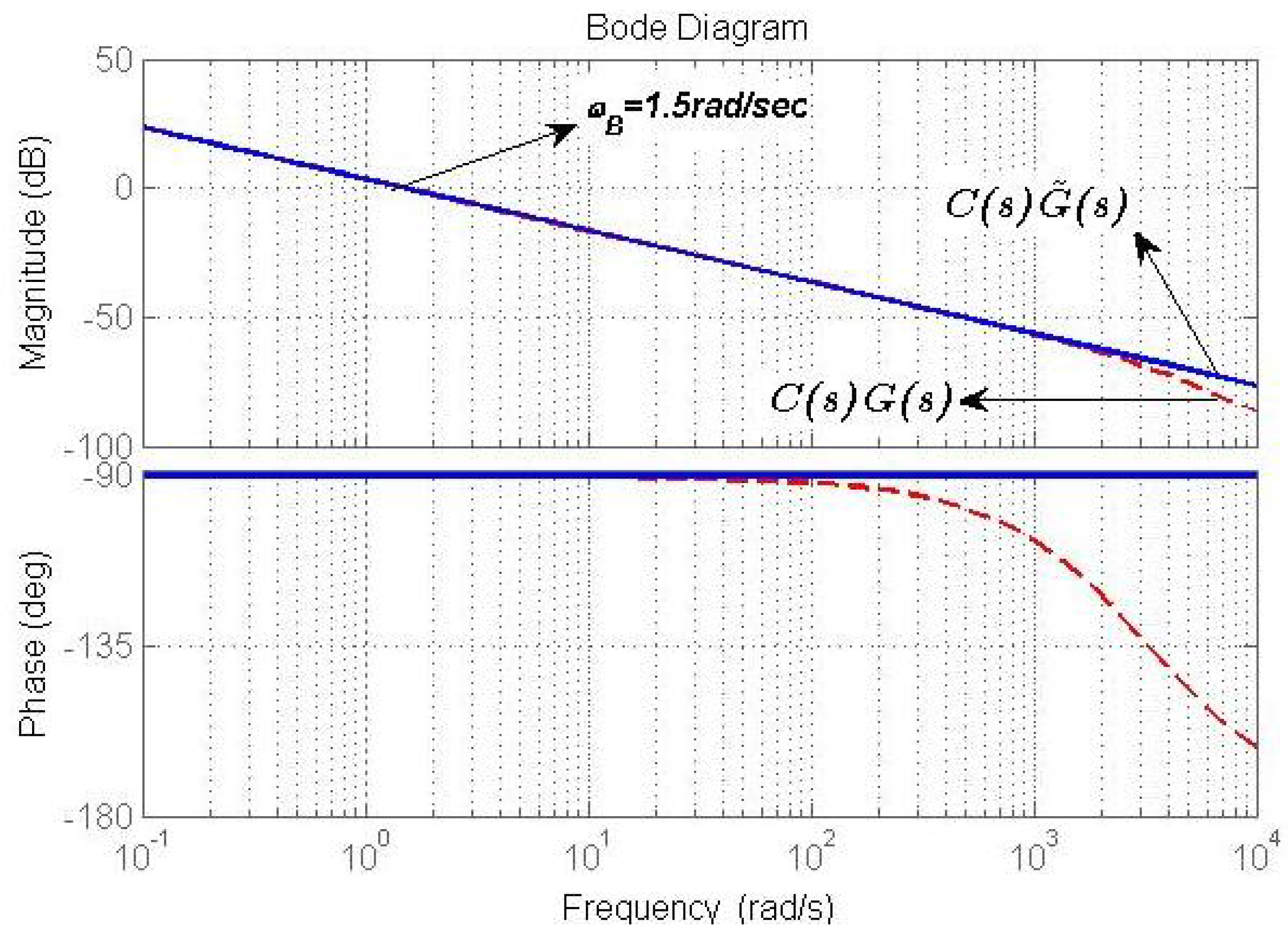
In Figure 14, the open loop Bode diagrams of $C\left(s\right)\tilde{G}\left(s\right)$ and $C\left(s\right)G\left(s\right)$ show that controller (39) satisfies the conditions of design, stability, and robustness for both the transfer function (22) and the simplified model (38). Therefore, conditions (i) of Lemmas 1 and 2 fulfilled.

The second step of the design according to condition (ii) of Lemmas 1 and 2 is the design of filter $F\left(s\right)$. As stablish in [30], it is necessary to calculate $\tilde{G}{\left(s\right)}^{-1}G\left(s\right)$ resulting in

$$\tilde{G}{\left(s\right)}^{-1}G\left(s\right)=\frac{3255}{\left(s+3255\right)}.$$

(40)

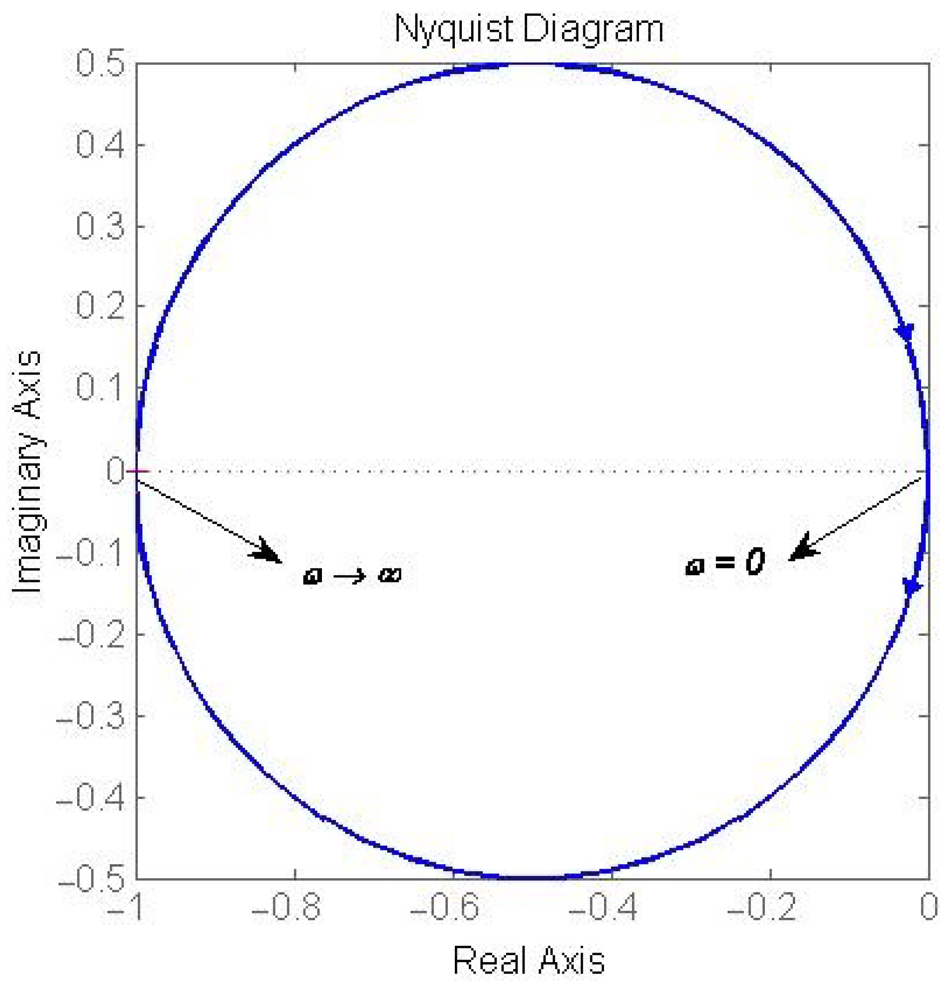
Because $\underset{\omega \to 0}{lim}\tilde{G}{\left(j\omega \right)}^{-1}G\left(j\omega \right)=1$ and $\underset{\omega \to \infty }{lim}\tilde{G}{\left(j\omega \right)}^{-1}G\left(j\omega \right)=0$, $H\left(s\right)$ will have zeros at zero and infinite. Also, because $\tilde{G}\left(j\omega \right)$ and $G\left(j\omega \right)$ are both stable and minimum phase, $H\left(s\right)$ is stable. 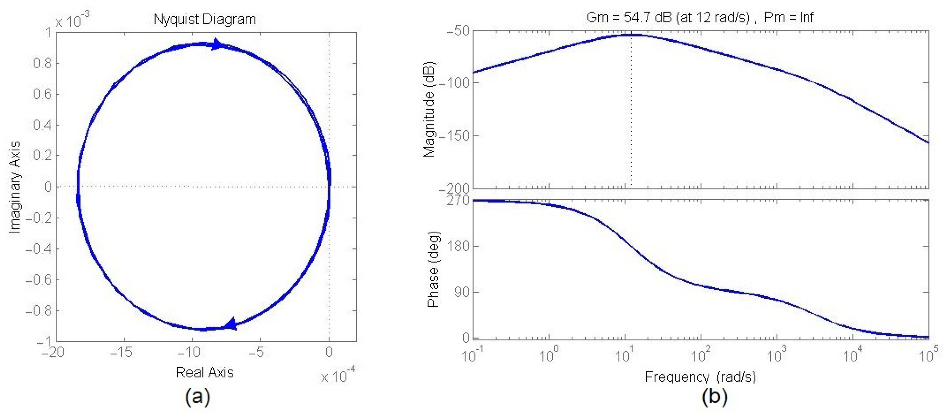In fact, $H\left(s\right)=-\frac{s}{\left(s+3255\right)}$ has a Nyquist plot, Figure 15, with no encirclements to point (−1,0).

Hence, to comply with condition (ii) of Lemma 1, filter $F\left(s\right)$ can be designed with arbitrary bandwidth ${\omega }_{B_F}$, provided $F\left(s\right)H\left(s\right)$ has adequate stability margin, as indicated by condition (ii) of Lemma 1. Additionally, the degree of $F\left(s\right)$ must assure $F\left(s\right){\tilde{G}}^{-1}\left(s\right)$ causal.

In this context, and because feedback controller $C\left(s\right)$ was designed satisfying a bandwidth ${\omega }_B$ = 1.5 rad/s, filter $F\left(s\right)$ is designed second order, so $F\left(s\right){\tilde{G}}^{-1}\left(s\right)$ is causal, and with a bandwidth ${\omega }_{B_F}\approx 10$ rad/s in order to reject sensor noise at frequencies above $\omega$ > 15 rad/s, resulting in

$$F\left(s\right)=\frac{1}{{\left(0.0833s+1\right)}^2}.$$

(41)

The Nyquist plot and Bode diagrams of $F\left(s\right)H\left(s\right)$, Figure 16, show no encirclements to point (−1,0) and stability margins of $M_g=54.7 d{B}^{\prime }s$ and $M_p\to \infty$. Hence, according to conditions (ii) of Lemmas 1 and 2, polynomial $B\left(s\right)$ is stable and robust.

6.1. Control System Implementation

Although the NRDOB_PI control system was designed in continuous time, due to the characteristics of the power driver described in Section 5, it has to be implemented digitally. Therefore, PI controller (39) and filter (41) were discretised assuming a sample period T = 0.005 s resulting in

$$C\left(z\right)=\frac{1.1223z-1.1217}{z-1};F\left(z\right)=\frac{0.0017z+0.0017}{z^2-1.8835z+0.8869}.$$

(42)

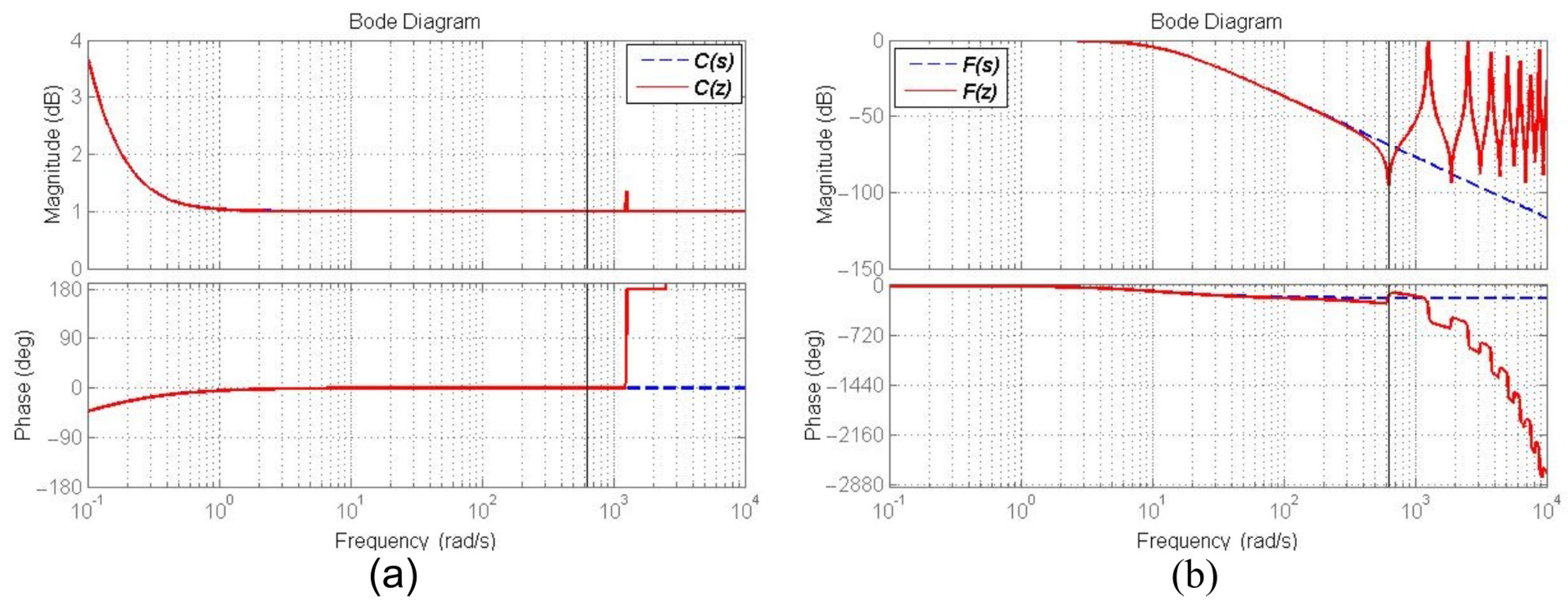
The sampling period was selected in order to maintain the filtering properties of $C\left(s\right)$ and $F\left(s\right)$ along a range of frequencies such that its discretization do not affect performance and stability of the control system, as exposed in Figure 17, where Bode diagrams of $C\left(s\right),C\left(z\right),F\left(s\right)$, and $F\left(z\right)$ show no significant differences well above the control system bandwidth of ${\omega }_B$= 1.5 rad/s.

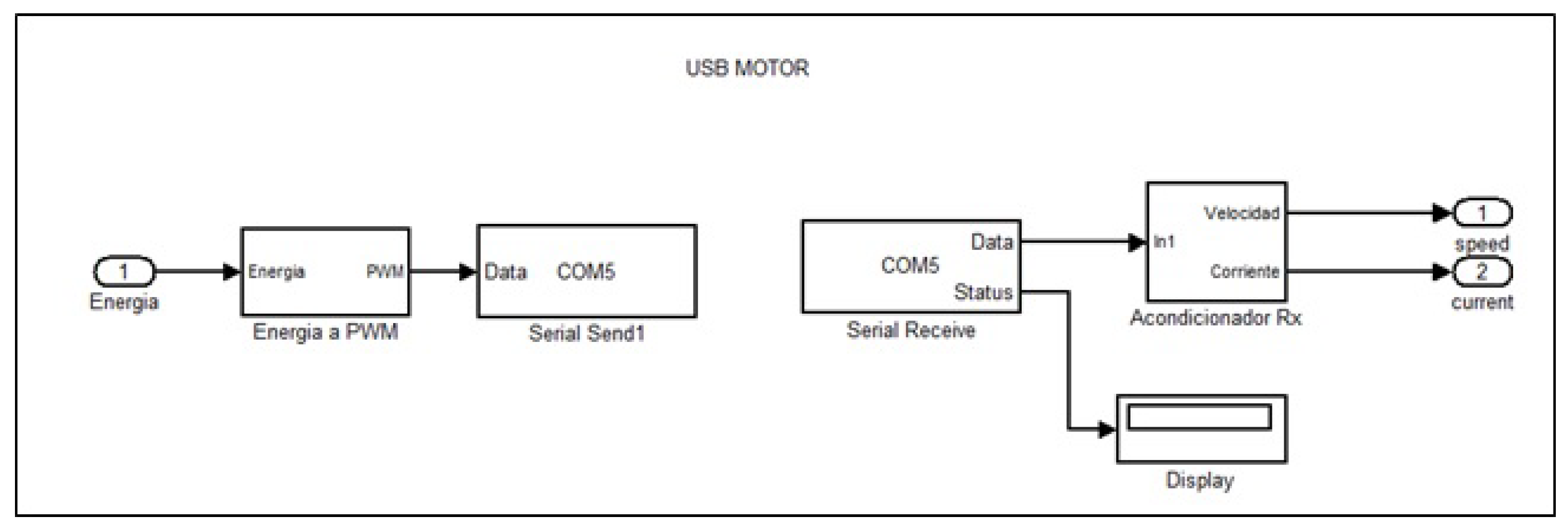
It is well known that saturation in conjunction with integral control actions affects the performance of any control system. Therefore, to reduce undesired effects of saturation in the control signal, an “anti-windup” scheme was implemented in addition to the PI controller and the NRDOB. In this case the maximum voltage and current provided by the power source are $\pm 50$ V and $\pm 3$ A, respectively. 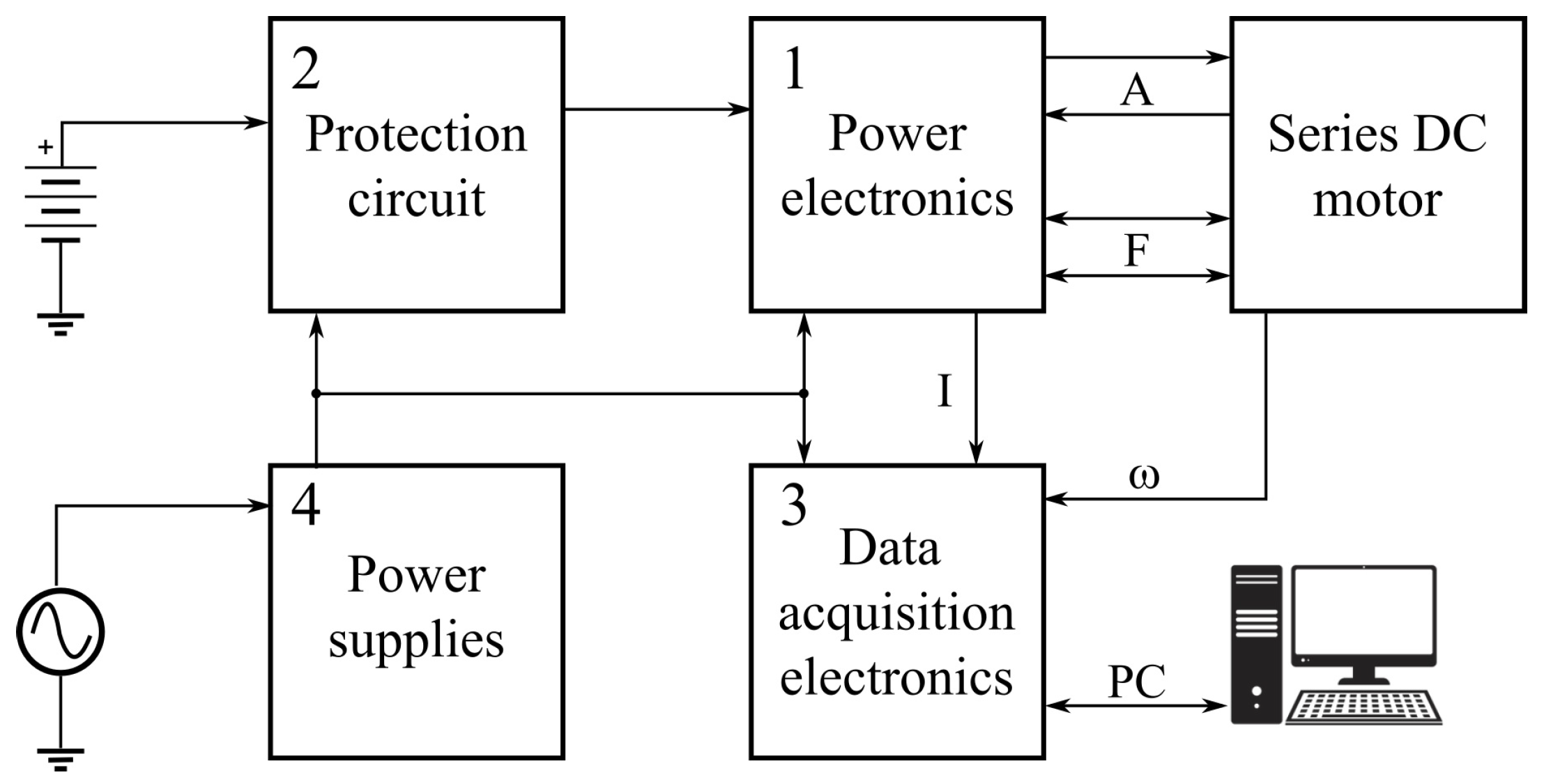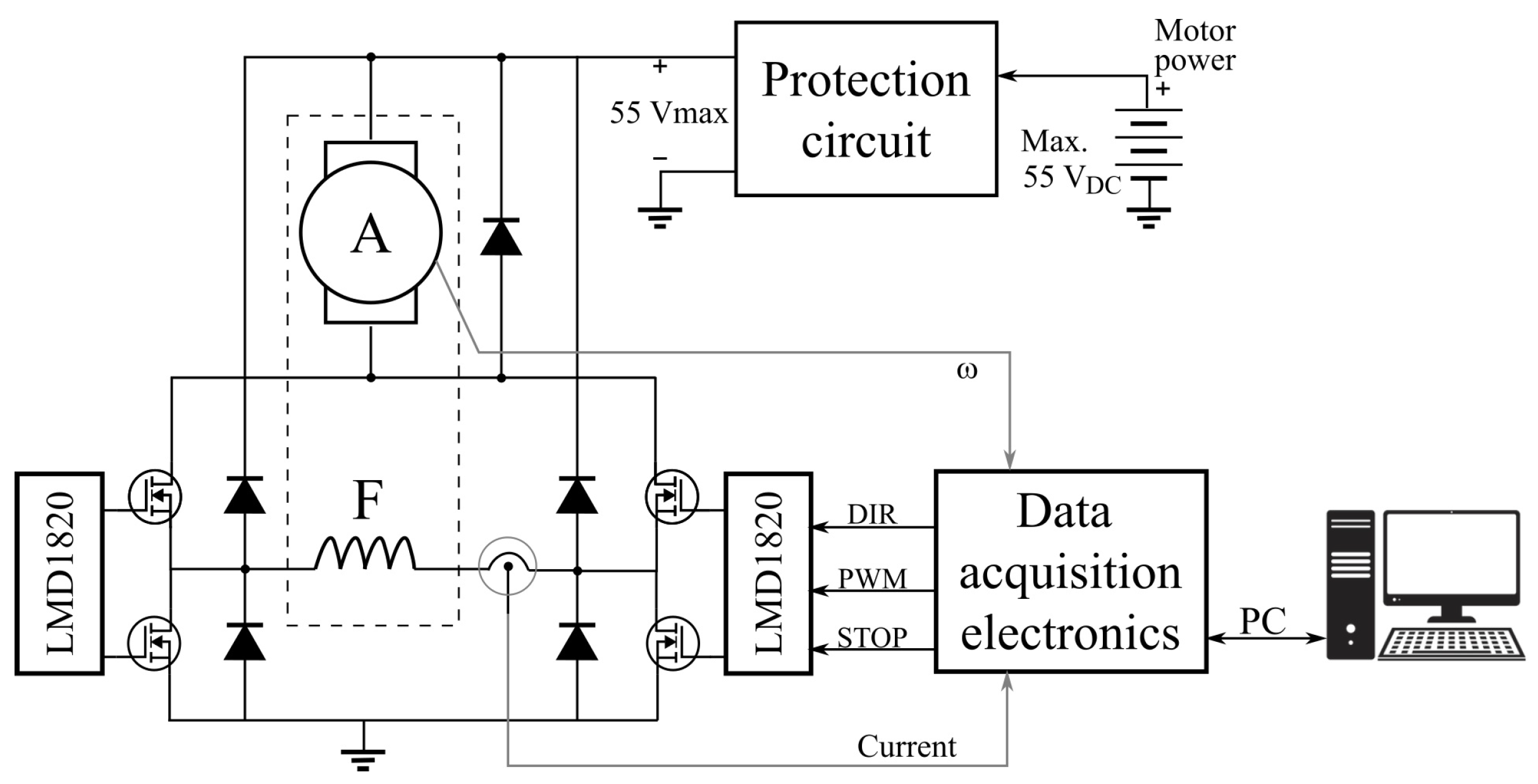The real-time SIMULINK program of the NRDOB_PI control system, including “anti-windup”, for the series DC motor is presented in Figure 18 and Figure 19.

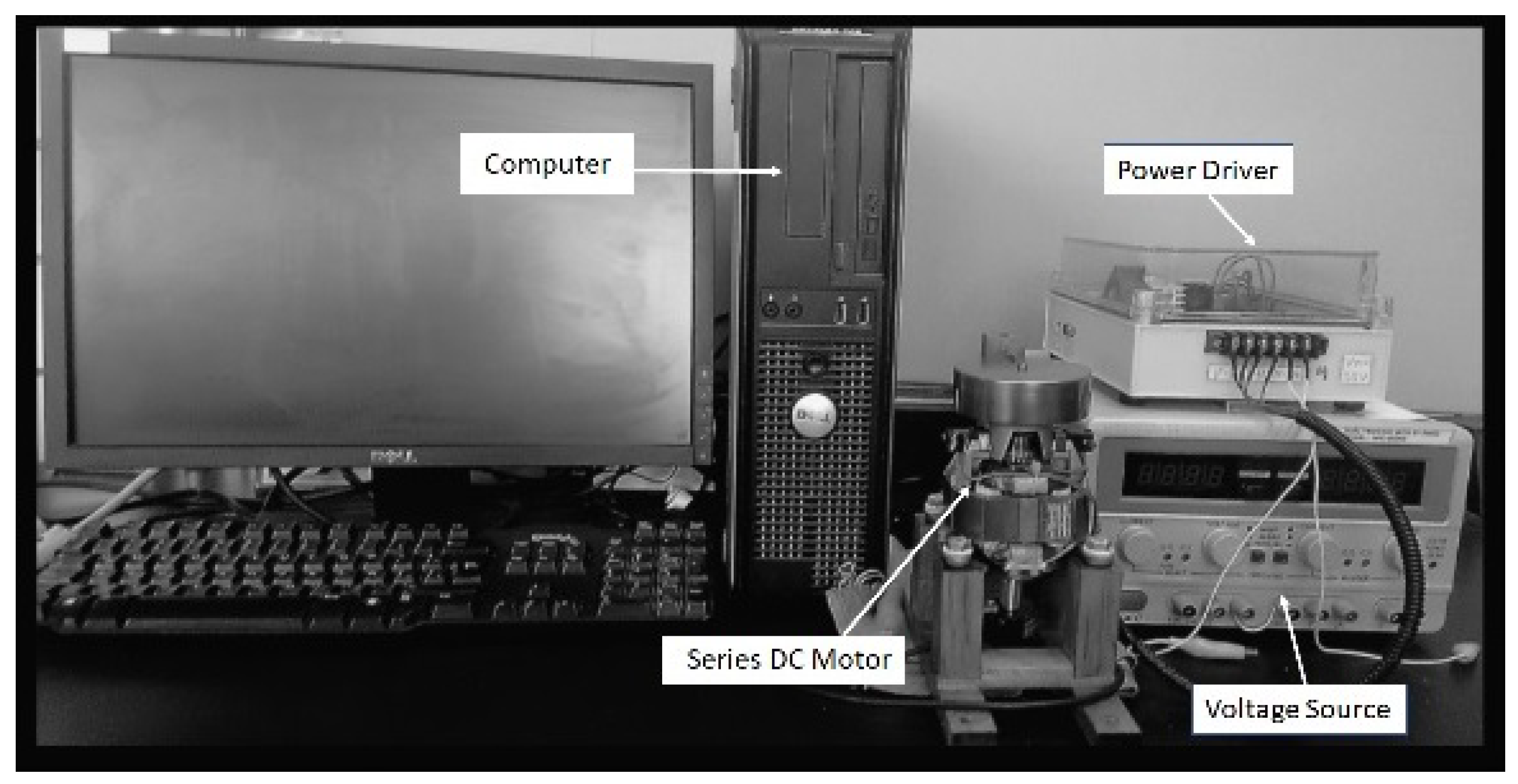
Finally, the experimental set-up of the NRDOB_PI speed control system for the series DC motor is shown in Figure 20.

6.2. Experimental Results

Different experiments were carried out varying reference signal $R\left(s\right)$ to assess the NRDOB_PI speed control system for the series DC Motor. They were selected in order to evaluate the capabilities of the control system under regulation and tracking conditions, suppression of the sensor noise effects and the effectiveness of the power driver to invert the polarization of the motor and consequently inverted motion and torque.

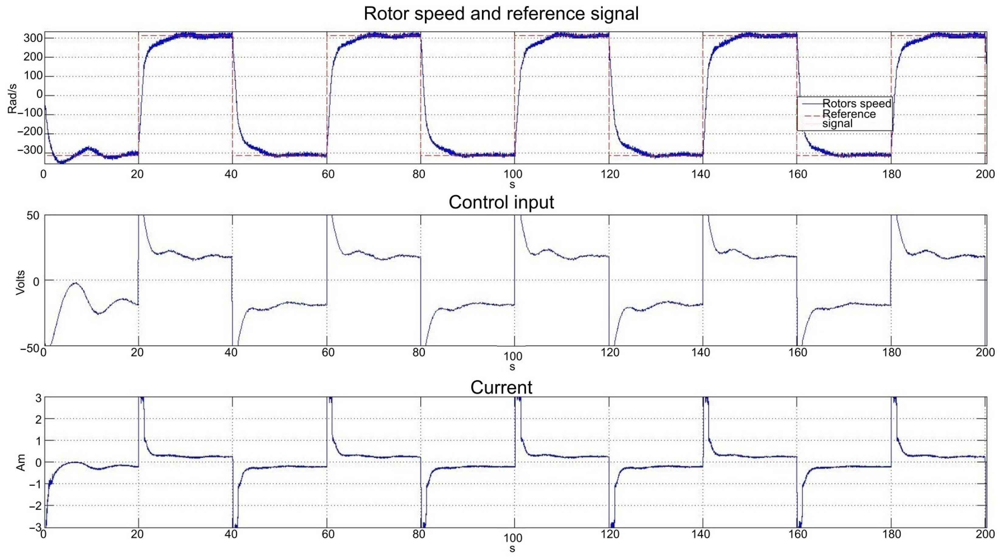
6.2.1. Response to a Square Reference Signal

In Figure 21, the response to a reference signal $R\left(s\right)$ given by a train of square pulses with amplitude $A=\pm 300$ and frequency $\omega$ = 150 rad/s shows that the power driver is capable of inverting motor polarity, so inverse motion—inverse torque—is achieved. Also, the effects of the sensor noise were highly reduced by the NRDOB, compared with those reported in [4], reducing control efforts. Moreover, the PI controller with the “anti-windup” scheme satisfies the conditions of design with very low current consumption. It should be noted that the peaks present in the control input and current are due to the extremely demanding sudden changes in $R\left(s\right)$.

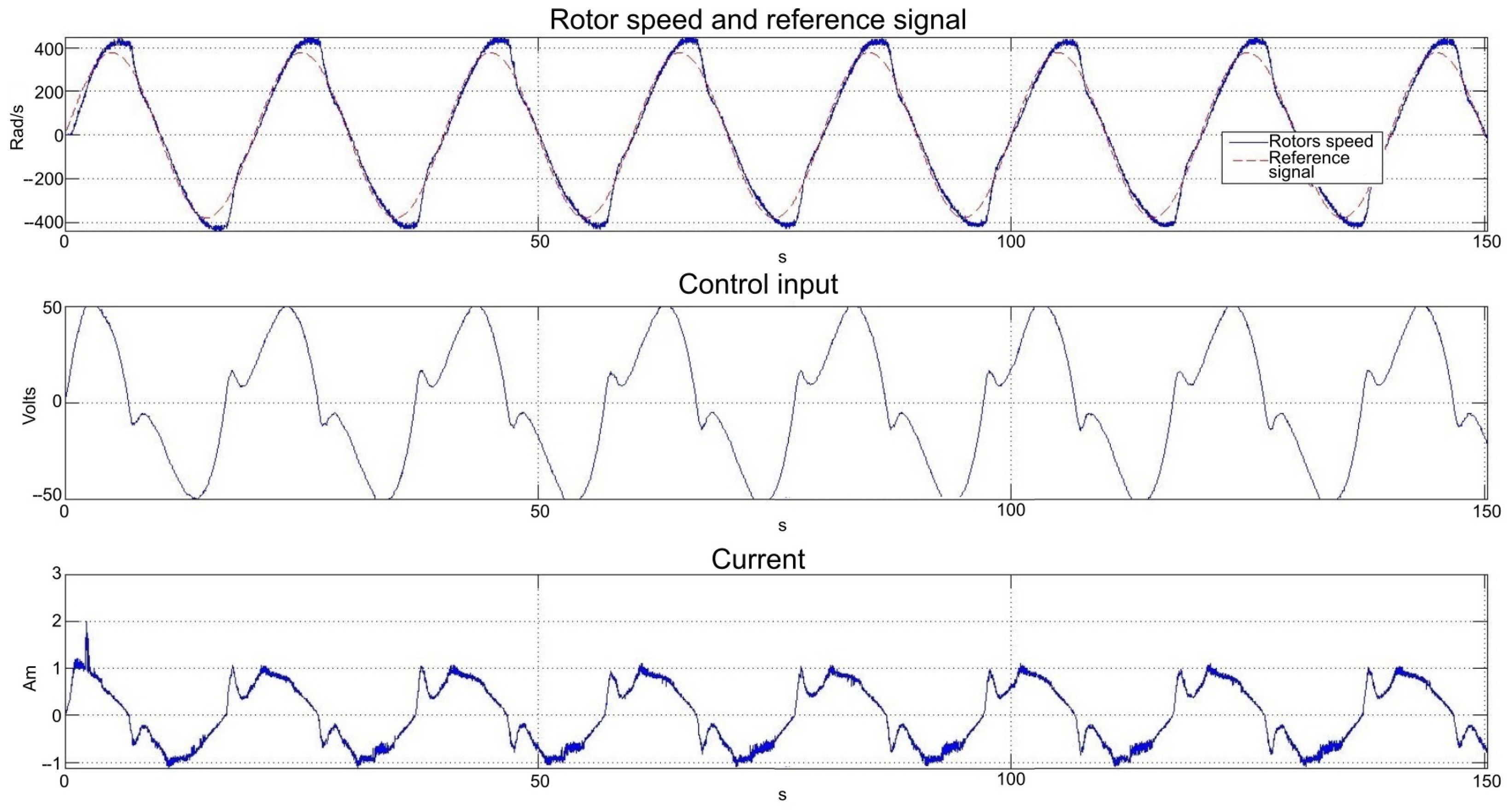
6.2.2. Response to a Sinusoidal Reference Signals

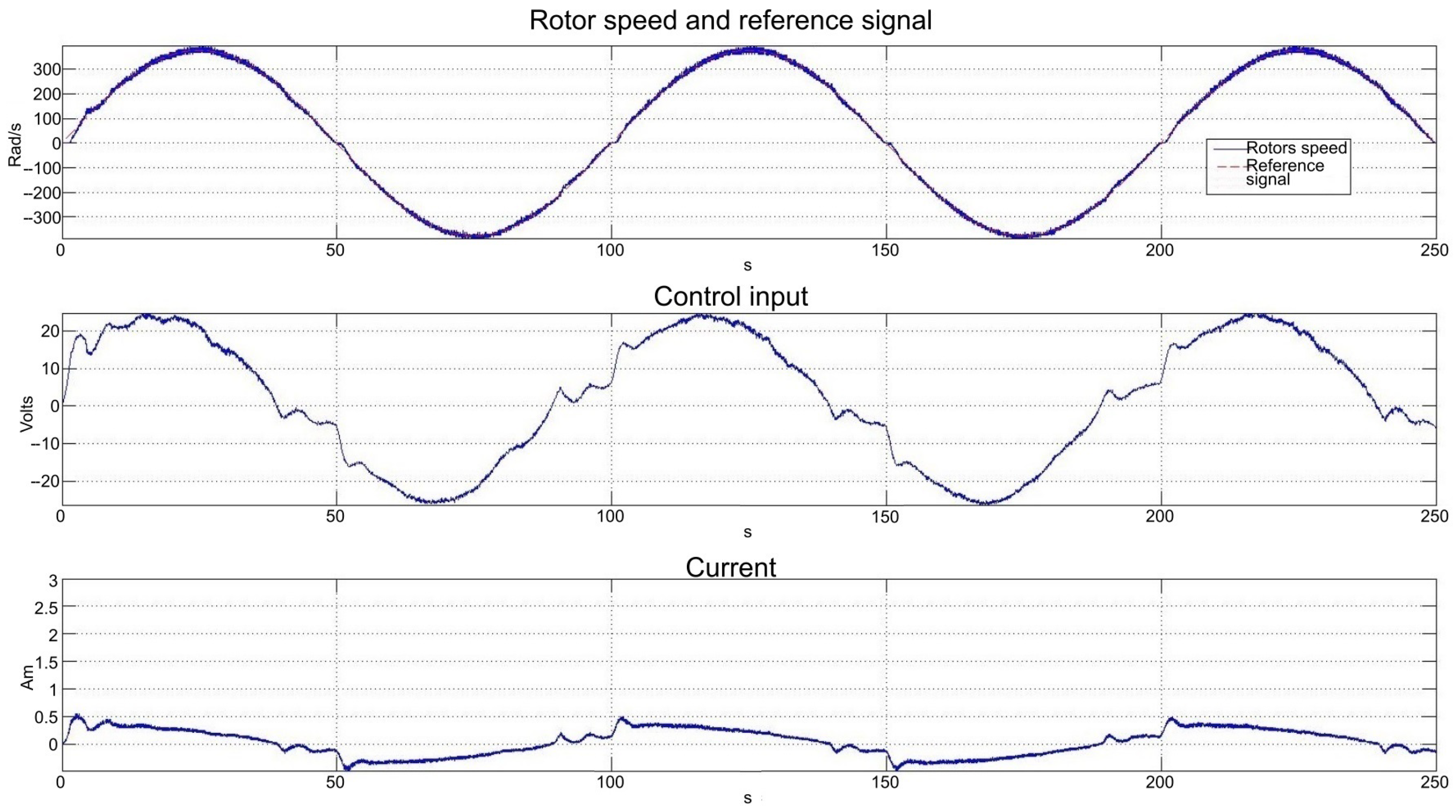
To assess NRDOB_PI control system performance under tracking conditions, two experiments were performed with two sinusoidal reference signals; the first when $R\left(s\right)$ = 380 sin(0.063t), at a frequency well below the control system bandwidth, and the second when $R\left(s\right)$ = 380 sin(0.31416t), relatively close the bandwidth control system. The two responses are shown in Figure 22 and Figure 23, respectively.

The responses to $R\left(s\right)$ = 380 sin(0.063t) show excellent tracking performance including inverse motion and low current consumption of $\pm 0.5$ A, whereas the responses to $R\left(s\right)$ = 380 sin(0.31416t) present a normal level of deterioration, as this reference signal pushes the control system close to its bandwidth, where its phase delay is more evident. Increasing reference signal frequency also increases control signal voltage and breaking effort with the consequent augmentation in current consumption, although it maintains acceptably low levels of around a maximum of $\pm 1$ A. In addition, the NRDOB properly filters and reduces sensor noise as anticipated.

6.2.3. Response to a “Sawtooth” Reference Signal

The responses to a “sawtooth” reference signal are shown in Figure 24, apart from allowing the assessment of the NRDOB_PI and the power driver to tracking a ramp-like signal, inversion of the direction of rotation and noise filtering, it exposes the “dead zone” of the series DC motor, due to inertias and friction present in many electromechanical devices. In spite of this highly non-linear characteristic, it does not deteriorate significantly the performance of the control system.

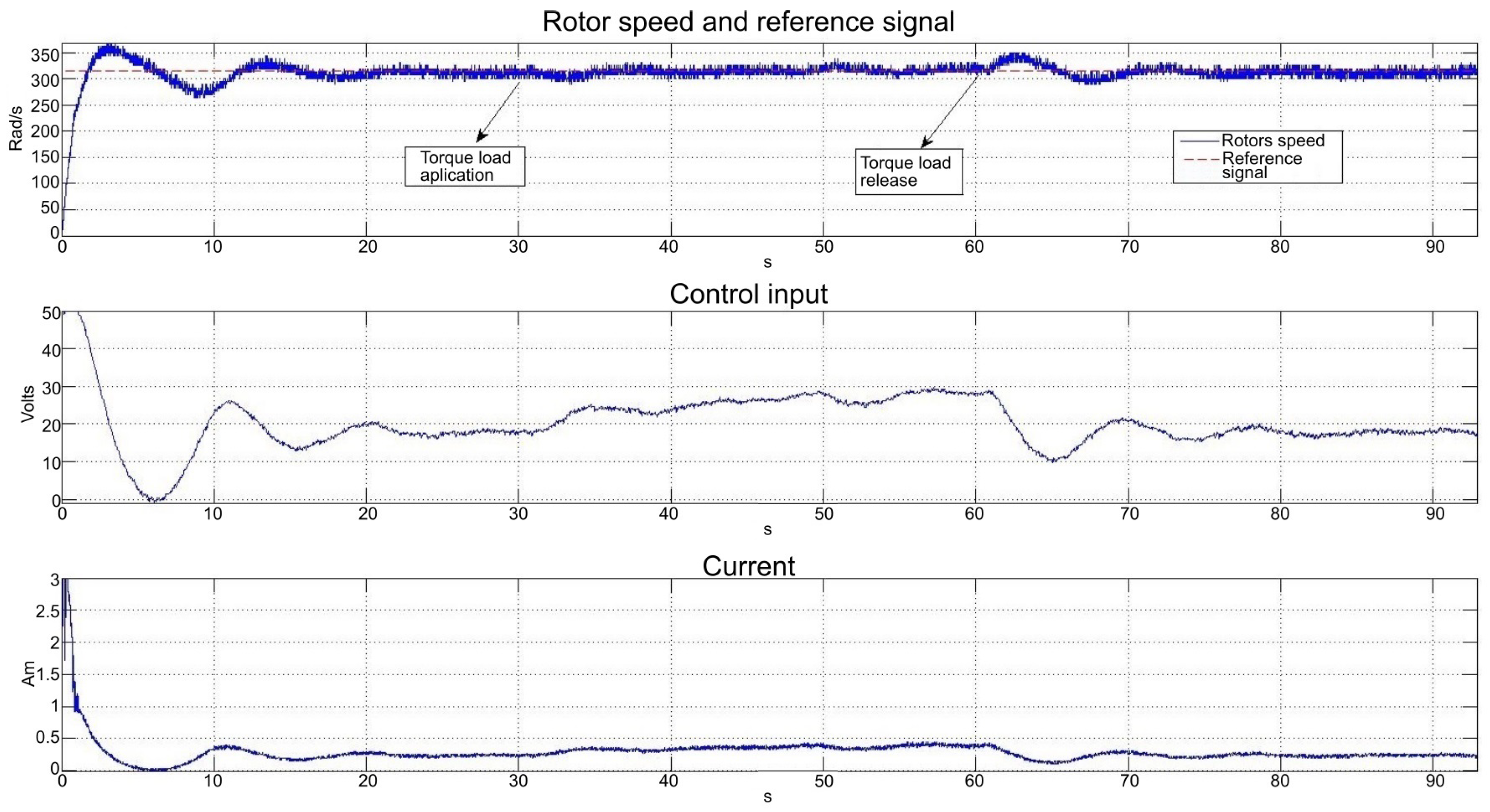
6.2.4. Response under Torque Load Perturbation

This final experiment seeks to assess NRDOB_PI control system under unknown load perturbations. The unknown load perturbation was applied at t = 30 s and released at t = 60 s when the reference signal is given by the constant $R\left(t\right)$ = 320 rad/s. As shown in Figure 25, control input (input voltage) shows an increment at t = 30 s to approximately 30 V, and a decrement to its previous value, before the perturbation injection, of around 20 V at t = 60 s. The same occurred with current consumption without a significant increment as its value remains below $0.5$ A, Therefore, as expected, the control system was able to reject the perturbation.

7. Conclusions

The design of a speed control system for a series DC motor has been presented. The approach followed makes use of the NRDOB, the classical PI controller and an anti-windup scheme. The control system design is based on the modelling of the series DC motor, including magnetic saturation and its linearization around an equilibrium point. Additionally, and to increase the performance of the control system, a power driver capable of inverting the polarization of the motor, and consequently the rotor direction of rotation and the induced magnetic torque, was designed and implemented. This article represents the third part of a series of reports regarding the speed control problem of series DC motors. In the previous reports, it was shown that a series DC motor, apart from its non-linear characteristics does not have a well-defined relative degree when rotor speed or current consumption is zero, so most non-linear controllers are not suitable when inverse motion is required. Also, as speed sensors introduce high frequencies, noise control efforts are increasingly unnecessary with the consequent increment in current consumption. Additionally, it was also shown that a power driver capable of inverting the induced magnetic torque is necessary to improve the performance of any control strategy for this kind of electric motor. Although many approaches have been proposed to overcome input/output perturbations, only the NRDOB copes directly with the problem of sensor noise without affecting or reducing performance. The design of the overall control system required to establish global conditions for stability and robustness for NRDOB-based control systems. This conditions, together with a methodology of design were established in a second report. Moreover, it was also shown that as the NRDOB is an internal model control strategy it is not necessary for the process model to match the process; in fact, under certain conditions a model not matching the process is required. Therefore, in this article the comprehensive design and implementation of the speed control system for a series DC motor is presented. The results here presented show that simple PI controllers in conjunction with NRDOB, which basically implies the design of a second order filter with unity steady-state gain, can overcome the problems associated not only with sensor noise and parametric uncertainty but also with the non-linear dynamics of the series DC motor. It is not a well-defined relative degree, resulting in a highly robust control system with excellent performance either in regulation or tracking conditions, in a wide range of operation, and torque load perturbations. Real-time experimental results proved that the designed power driver can invert the polarization of the motor not only in a safe manner but with excellent switching speed.