Local Path Planning of the Autonomous Vehicle Based on Adaptive Improved RRT Algorithm in Certain Lane Environments

Abstract

Given that the rapidly exploring random tree algorithm (RRT) and its variants cannot efficiently solve problems of path planning of autonomous vehicles, this paper proposes a new, adaptive improved RRT algorithm. Firstly, an adaptive directional sampling strategy is introduced to avoid excessive search by reducing the randomness of sampling points. Secondly, a reasonable node selection strategy is used to improve the smoothness of the path by utilizing a comprehensive criterion that combines angle and distance. Thirdly, an adaptive node expansion strategy is utilized to avoid invalid expansion and make the generated path more reasonable. Finally, the expanded ellipse is used to realize vehicle obstacle avoidance in advance, and the post-processing strategy removes redundant line segments of the initial path to improve its quality. The simulation results show that the quality of the planned path is significantly improved. This path followed successfully has good trajectory stability, which shows the proposed algorithm’s effectiveness and practicability in autonomous vehicles’ local path planning.

1. Introduction

As a kind of wheeled mobile robot, an autonomous vehicle plays an essential role in reducing traffic accidents, easing traffic jams, improving traffic efficiency, etc. [1]. The autonomous vehicle is typically capable of recognition, decision making, and tracking control [2,3,4,5]. As a critical component of autonomous driving, path planning has become a popular research topic. Path planning is defined as finding a collision-free path from the initial state to the target state in a configuration space where obstacles can be seen [6,7].

Up to now, many algorithms regarding path planning have been presented. The artificial potential field method is a virtual force method whose basic idea is to design the movement of autonomous vehicles under the combined force of an attractive force generated by the target point and a repulsion force generated by the obstacle [8]. This method is simple to compute, and the planned path is safe and feasible, but it is easy to fall into the local minimum trap, that is, the local minimum point [9,10,11]. The algorithm combining the artificial potential field method and the elastic band model can gain an ideal path when applied to vehicle path planning [12]. Nevertheless, its computation model is complex, resulting in low search efficiency. Dijkstra algorithm and A* algorithm can obtain the shortest path in rasterized environments, but the generated path consists of broken lines, which leads to poor smoothness [13,14,15]. The rapidly exploring random tree algorithm (RRT), a typical sampling-based method, is a single-query motion path planning algorithm. Its advantages include probability completeness, low computational cost, a natural extension for non-holonomic constraints, and simple environment modeling [16,17,18]. However, it has the disadvantages of a slow convergence rate, low path planning efficiency, and its planned path may be inefficient [19,20,21].

Regarding the disadvantages of the RRT algorithm, many scholars have carried out various improvements. The biased-RRT algorithm is proposed to reduce sampling blindness by sampling the target point with a certain probability [22]. The bi-direction RRT algorithm enhances the exploration of the unknown area, in which two random trees grow in parallel from the starting point and the target point, respectively, until the line segment of their extended nodes does not collide with obstacles [23]. The RRT-connect algorithm is a variant of the bi-direction RRT based on the greedy algorithm, extending their nodes as much as possible without encountering obstacles [24]. These three algorithms enhance the speed of path planning, but the path lengths derived by them are not optimal. As a supplement, RRT* can provide a quasi-optimal path while requiring a large amount of node backtracking to judge the constraints, but its convergence speed is affected to some extent [25]. The improved RRT algorithms based on the boundary of obstacles make the RRT algorithm effectively applicable to the complex environment with narrow channels [26]. Gan et al. propose an improved RRT algorithm that utilizes a 1–0 biased-goal method to change probability biased to the target different from the RRT and the biased RRT, resulting in having shorter computational time and path length [27]. Chen et al. employ a quadruple tree mechanism and the method of adding guidance to improve the RRT-connect algorithm, which speeds up the search of the algorithm [28]. Ge et al. utilize the force direction of the potential field to determine the search direction of the sampling space of the bidirectional RRT* algorithm, which improves both the probability integrity and the search efficacy [29]. The above algorithms have improved the quality of the path, such as path length and computation time when applying in unstructured environments, but seldom consider the characteristics of structured road environments. In addition, path smoothness is also vital to the autonomous vehicle with non-holonomic constraints. Kuwata et al. adopt a Dubins curve, which is composed of straight lines and arc lines, to generate a path, but the curvature of the generated path is discontinuous [30]. Lau et al. use the five-times Bessel curve to generate a path without considering the continuity of path curvature and the self-constraints of mobile robots [31]; as a result, this obtained path is not followed well. Thanh et al. employ a modified RRT to generate a sub-optimal path and then use fourth-order non-uniform B-splines and the interior-point optimizer method to optimize that path to obtain excellent tracking performance [32].

Therefore, this article proposes an adaptive improved RRT algorithm to obtain a path considering vehicle constraints and applying it to structured road environments. The improved path planning algorithm has made contributions to collision detection, node sampling, nearest node selection, node extension, and path optimization.

• This method uses the sampling node method based on heuristic information to make the random tree grow more directionally and utilizes the adaptive sampling space and the adaptive step size to speed up its convergence.
• The road environment constraints and the vehicle’s constraint method gained by a magnifying mechanism considering the motion characteristics of the vehicle are considered to make the vehicle achieve an excellent behavior of avoiding obstacles.
• A heuristic node selection mechanism is introduced to select the nearest tree node so that the vehicle moves smoothly at less cost.
• The post-processing, including the pruning method and the cubic B-spline, is used to optimize the generated path to make the path satisfy the requirement of autonomous vehicle driving.

The article is organized as follows: Section 2 discusses the road environment and the non-integrality constraint of the vehicle to construct constraints of path planning. The adaptive improved algorithm is presented in Section 3. Experiments and results for demonstrating the relevant performance of various algorithms and the superiorities of the proposed algorithm are offered in Section 4, and the conclusions are provided thereafter.

2. Preliminaries

In this section, we introduce the road environment method of path planning and design the constraints of the road environment. Furthermore, the vehicle model with non-integrality constraint is presented to prove that the steering constraint of the vehicle should be taken into account in the growth of the random tree.

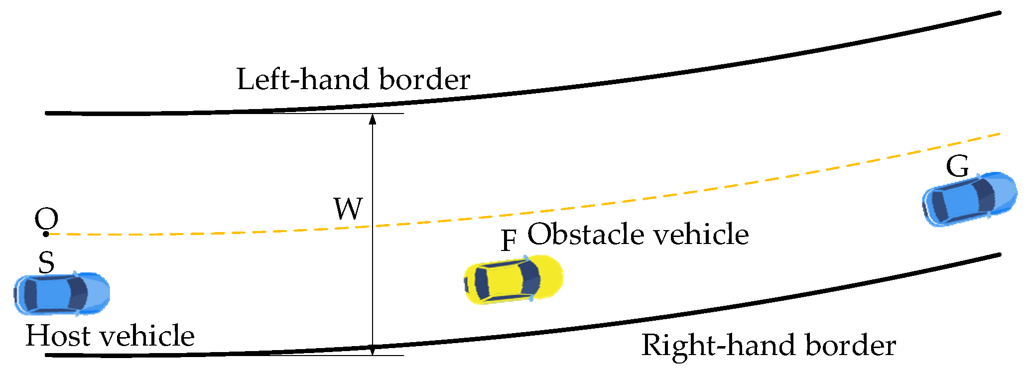
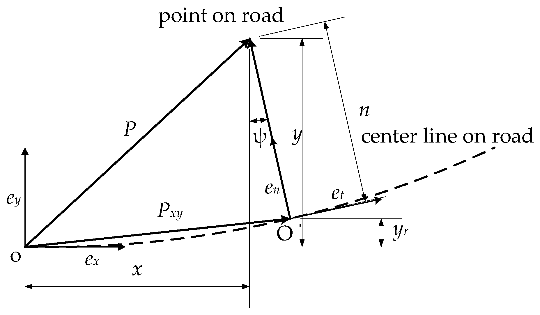
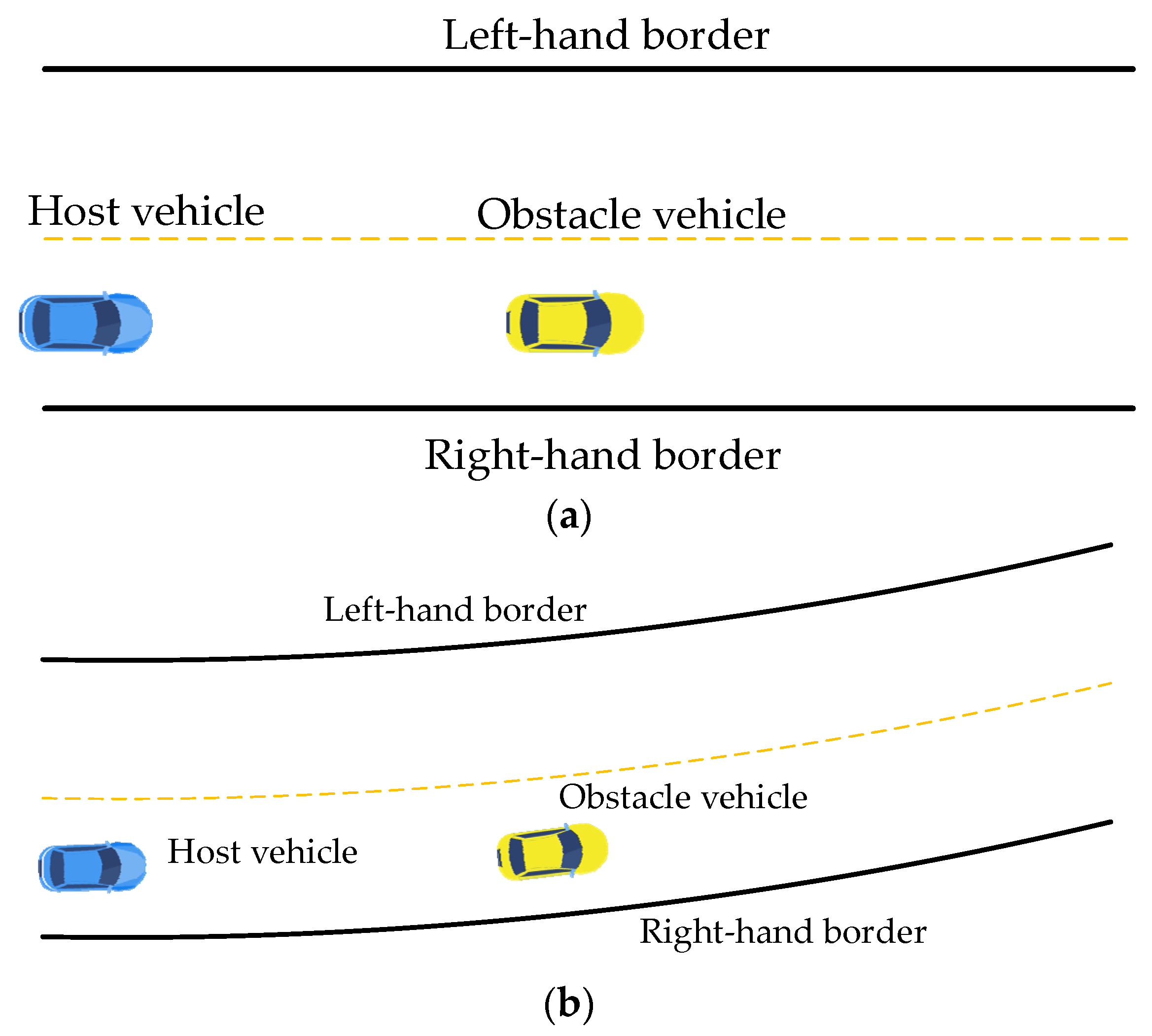
2.1. Road Environment Method

2.1.1. Road Environment Geometries

The road environments consisting of a straight road environment and a curved road environment are established after obtaining the surrounding road information. The straight road environment can be established directly according to the road length and width. As to the curved road environment shown in Figure 1, S is the starting point of planning, F is the location point of the obstacle, G is the target point of planning, W is the width of the road, and the origin O of the road reference coordinate frame is defined as a point on the road center line. A cubic equation of one variable can construct the center-line of the road to meet the curvature requirements [12], which is given by

$$y_r=A{x}^3+B{x}^2+Cx+D$$

(1)

where $y_r$ represents the value of the $y$ axis and $x$ represents the horizontal distance from the origin O. $A$, $B$, $C$ and $D$ are parameters of the equation. The position vector $P_{xy}$ of the road center line, as described in Figure 2, is given by

$$P_{xy}=x{e}_x+y{e}_y$$

(2)

Under the boundary conditions $y(0)=0$ and $y\prime \left(0\right)=0$, the unit tangent vector and unit normal vector of a point on the center line of the road can be represented by Equations (3) and (4), respectively. Thus, the points on the left and right boundaries of the road can be represented by Equation (5), and any point on the road can be represented by Equation (6).

$$e_t=\frac{1}{\sqrt{1+{y\prime }^2}}{e}_x+\frac{y\prime }{\sqrt{1+{y\prime }^2}}{e}_y$$

(3)

$$e_n=\frac{-y\prime }{\sqrt{1+{y\prime }^2}}{e}_x+\frac{1}{\sqrt{1+{y\prime }^2}}{e}_y$$

(4)

$$B_{xy}=P_{xy}\pm \frac{W}{2}{e}_n$$

(5)

$$P=x{e}_x+y{e}_y=P_{xy}\pm n{e}_n$$

(6)

where $W$ is the width of the road and $n$ is the scalar value along the unit normal vector $e_n$. Considering that the included angle between the tangent of the road curve and the $x$ axis of the road reference coordinate frame is minimal, we can assume $n=y-y_r$. Thus, the position vector of a point on the road can be approximately expressed as:

$$P=P_{xy}+(y-y_r)e_n$$

(7)

2.1.2. Constraints of Road Environment

To be followed effectively by an autonomous vehicle, a path must meet constraints of the road environment when planning; in other words, the growth of the random tree must meet constraints of the road environment. Equation (8) expresses the conditions to be satisfied by the random tree nodes.

$$\{\begin{array}{l}{P}_{star{t}_x}\le Tree{(\mathrm{i})}_x\le P_{goa{l}_x}\\ B_{right}-\frac{D}{2}\le Tree{(\mathrm{i})}_y\le B_{left}+\frac{b}{2}\end{array}$$

(8)

where $P_{start}$ is the starting point, $P_{goal}$ is the goal point, $B_{left}$ and $B_{right}$ are the left and the right borders of the road, respectively, and $b$ is the width of the vehicle.

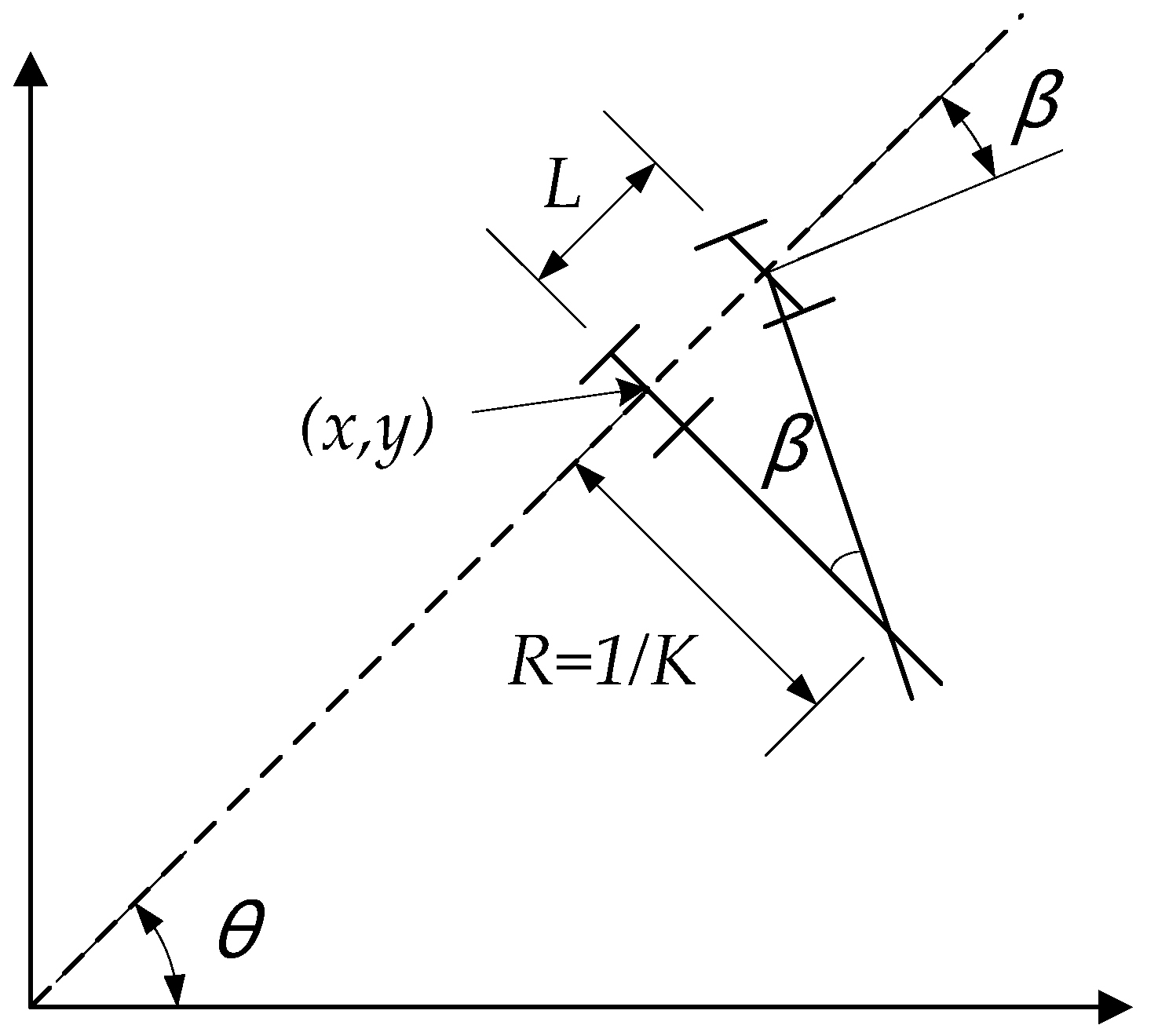
2.2. The Vehicle Model with Non-Integrality Constraint

To deal with the path tracking problem, the non-integrality constraint of the vehicle must be considered. A simplified vehicle model is shown in Figure 3 [33]. Owing to pure rolling of the wheel in the plane, the speed direction of the vehicle body must point to its main axis at any moment of motion, that is, to meet Equations (9) and (10).

$$dy\cos \theta -dx\sin \theta =0$$

(9)

$$K_{\max }=\frac{\tan {\phi }_{\max }}{L}=\frac{1}{R_{\min }}$$

(10)

where $(x,y)$ is the position of the vehicle mass center in the reference coordinate frame, $\theta$ is the included angle between the vehicle longitudinal axis and the $x$ axis of the reference coordinate frame, $\beta$ is the steering angle of the vehicle front wheel and $\left|\beta \right|\le {\beta }_{\max }$.

Through the above analysis, the steering radius of the vehicle needs to be considered in the extension of the tree nodes.

3. Adaptive Improved RRT Path Planning

3.1. Basic RRT

The RRT algorithm gradually builds a path from the starting point regarded as the root node of the random tree to the target point by searching the feasible region space and then iteratively adding new randomly selected nodes as leaf nodes toward the region of the target point.

Algorithm 1 shows the basic RRT algorithm. The random sampling point $P_{rand}$ is generated by the $\mathrm{RANDOM}\_\mathrm{STATE}$ function. Among the existing tree nodes, the one nearest to $P_{rand}$ is selected as the extension node $P_{near}$ by the $\mathrm{NEAREST}\_\mathrm{NEIGHBOR}$ function, and a line is drawn to connect $P_{rand}$ and $P_{near}$. $P_{new}$ is generated in the direction of this line by the $\mathrm{EXTEND}$ function. Then, if there is no collision between the obstacle and the line between $P_{near}$ and $P_{new}$, the latter is added to the random tree as a new leaf node. The above processes is repeated, and the search is ended when the distance between $P_{new}$ and $P_{goal}$ is less than the threshold $D_{\lim it}$. Finally, the planned path is generated by the $\mathrm{GET}\_\mathrm{PATH}$ function, as shown in Algorithm 2.

Algorithm 1:$\mathrm{Build}\_\mathrm{RRT} (P_{init}$)

$1. \mathrm{T}\_\mathrm{init} (P_{init}$)

$2. \mathrm{While} \mathrm{DISTANCE} (P_{new}$$,P_{goal}$) do

$3. P_{rand}$←RANDOM_STATE ( )

$4. P_{near}$←$\mathrm{NEAREST}\_\mathrm{NEIGHBOR} (\mathrm{T}, P_{rand}$)

$5. P_{new}$←$\mathrm{EXTEND} (\mathrm{T}, P_{rand}$$, P_{near}$)

$6. \mathrm{if} \mathrm{DISTANCE} (P_{new}$$, P_{goal}$$)\le D_{\mathrm{l}\mathrm{i}\mathrm{m}it}$ then

7. Return T

8. endif

9. endWhile

10. path←GET_PATH (T)

Algorithm 2: Function GET_PATH (T)

1. Var path_set; $2. \mathrm{path}\_\mathrm{set}.\mathrm{Add}\_\mathrm{Node} (\mathrm{T}{.\mathrm{node}}_{\mathrm{n}}$); 3. while 4.         i←$\mathrm{Pre}\_{\mathrm{Node}\_\mathrm{Index}}_{\mathrm{n}}$; $5. \mathrm{path}\_\mathrm{set}.\mathrm{Back}\_\mathrm{Add}\_\mathrm{Node} (\mathrm{T}{.\mathrm{node}}_{\mathrm{i}}$); 6.         if i = 1 7.             break; 8.         endif 9.         i←i + 1; 10. endwhile 11. path←path_set

The result of the basic RRT algorithm applied to the vehicle path planning is shown in Figure 4. The green lines represent all branches of the random search tree, and the red line represents the planned path from the starting point (0, −1.875) to the target point (120, −1.875). From this graph, we can find that the random search tree attempts to explore the entire road space due to uniformly random sampling and a fixed extension step, which results in too many redundant searches and means that this planned path cannot be tracked by the vehicle because of significant changes in curvature. What is more, it is easy to cause instability or collision with obstacles in the driving process when the vehicle starts avoiding the obstacle close to it.

3.2. Adaptive Improved RRT Algorithm

Based on the above analysis of vehicle path planning problems caused by using the basic RRT algorithm, this paper proposes a different RRT variant applying to the local path planning of the autonomous vehicle. The adaptive improved RRT algorithm aims to generate an initial path quickly and then improve the quality of the initial path in the allowed time to meet the requirements of vehicle driving. Compared with the basic RRT, plenty of novel heuristics are discussed in collision detection, state sampling, node selection, node expansion, and path post-processing to optimize the algorithm’s performance suitable for vehicle path planning. Algorithm 3 shows the algorithm process of the adaptive improved RRT.

Algorithm 3:$\mathrm{Build} \mathrm{Adaptive} \mathrm{Improved}\_\mathrm{RRT} (P_{init}$)

$1. \mathrm{T}.\mathrm{init} (P_{init}$)

$2. \mathrm{While} \mathrm{DISTANCE} (P_{new}$$,P_{goal}$$)>D_{\mathrm{l}\mathrm{i}\mathrm{m}it}$ do

$3. P_{rand}$←EFFECTIVE_RANDOM_STATE ( )

$4. P_{near}$←EFFECTIVE_NEAREST_NEIGHBOR ( )

$5. P_{new}$←EFFECTIVE_EXTEND ( )

$6. \mathrm{if} \mathrm{COLLISION}\_\mathrm{DISTANCE} (P_{new}$$,P_{goal}$$) \le D_{\mathrm{l}\mathrm{i}\mathrm{m}it}$ then

7. Return T

8. endif

9. endWhile

10. path←GET_PATH (T)

11. path←PRUNING (path)

12. trajectory←SMOOTHING (path)

Path planning is described in the adaptive improved RRT algorithm to find a feasible passage from the starting point to the goal point. The random tree is initialized from the starting point. A novel $\mathrm{EFFECTIVE}\_\mathrm{RANDOM}\_\mathrm{STATE}$ function aims to make the sampling states more directional. The $\mathrm{EFFECTIVE}\_\mathrm{NEAREST}\_\mathrm{NEIGHBOR}$ function considering the vehicle’s non-integrality constraint is used to guide the random tree growth. Furthermore, the $\mathrm{EFFECTIVE}\_\mathrm{EXTEND}$ function is employed to help the random tree grow more flexibly. In each iteration, the $\mathrm{COLLISION}\_\mathrm{DISTANCE}$ function is used to evaluate whether the new point has reached the goal point. When the new point reaches the goal point, the $\mathrm{GET}\_\mathrm{PATH}$ function will find a broken line connecting the starting point and the goal point. Afterward, the $\mathrm{PRUNING}$ function removes redundant connecting lines based on the included angle constraint to obtain a feasible path after smoothing by the $\mathrm{SMOOTHING}$ function. The specific details of all heuristics are described below.

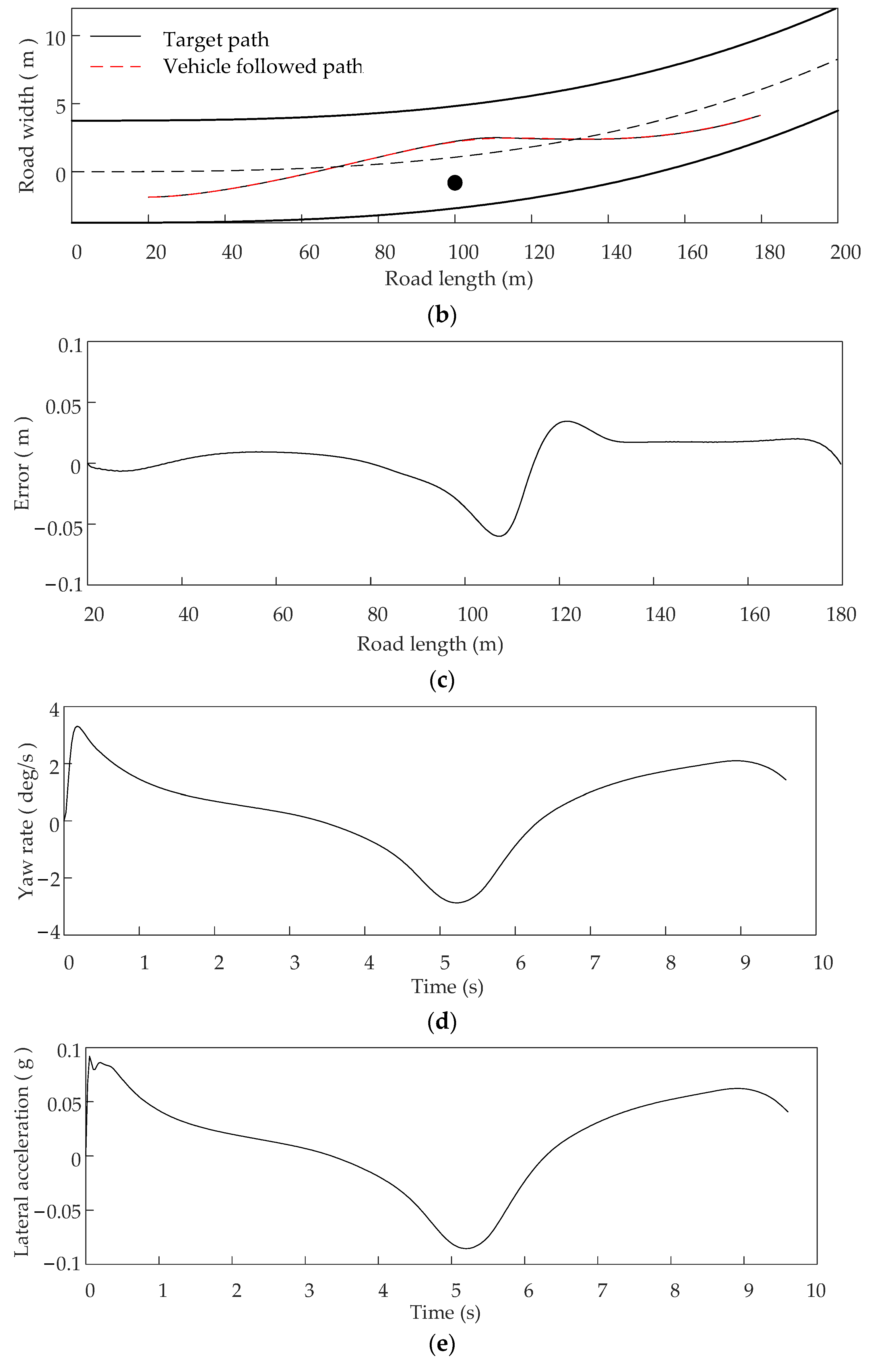
3.2.1. Collision Detection

In order to avoid the collision between the host vehicle and the obstacle vehicle, we use the secure ellipse method, which is scaled up appropriately to envelope the obstacle vehicle. What is more, we add the distance of advanced obstacle avoidance adjusting according to the host vehicle’s speed to the semi-major axis of the ellipse to make the impact of the obstacle vehicle on the host vehicle occur at a longer distance, as shown in Figure 5. If the tree node expanded by the random tree does not intersect with the expanded safety ellipse, that is, the connecting line between the new node and its parent node does not intersect with the obstacle vehicle, the newly extended node meets the requirements of the obstacle avoidance. Equation (11) shows that the new node does not collide with the expanded safety ellipse.

$$\frac{{(x-x_{ob})}^2}{{\left[s\cdot \left(\frac{v^2}{2\cdot \mu \cdot g}+a\right)\right]}^2}+\frac{{\left(y-y_{ob}\right)}^2}{{\left(s\cdot b\right)}^2}>1$$

(11)

where $(x,y)$ is the point on the line between the new node and its parent node, $(x_{ob},y_{ob})$ is the position of the obstacle vehicle, $a$ is the half-length of the obstacle vehicle, $s$ is the expansion coefficient of the safety ellipse, $v$ is the speed of the host vehicle, $\mu$ is the friction coefficient, and $g$ is the acceleration of gravity.

The secure ellipse is not only an easy and effective collision detection method but also ensures that the host vehicle can stay away from the obstacle vehicle in the corresponding driving direction at a safe distance.

3.2.2. Adaptive Directed Sampling Strategy

The basic RRT uses uniform random sampling to explore the entire sampling space, which will cause lots of unnecessary searches and a low convergence rate. To solve this problem, a novel heuristic mechanism, including the adaptive sampling space and the dynamic sampling method, is introduced to process the selection of the sampling space and random sampling states to improve search efficiency. It can make the random tree grow toward the target point and make the distance of the generated path from the reference trajectory small as possible.

Adaptive Sampling Space

The status of the local path planning of the autonomous vehicle during the driving process determines that its driving state is forward. Consequently, we introduce a method of the adaptive sampling space to obtain $P_{nearest}$ that is the node closest to the target on the random tree and then form an adaptive sampling space between the nearest tree node $P_{nearest}$ and the target point $P_{goa\mathrm{l}}$, which can avoid unnecessary searches in the area where the random tree has grown to improve the search efficiency. Equation (12) is the expression for this method.

$$\{\begin{array}{l}S\mathrm{a}\mathrm{m}\mathrm{p}\mathrm{l}\mathrm{e}\underset{\_}{}{\mathrm{zone}}_x=\left|P_{goa{\mathrm{l}}_x}-P_{neares{t}_x}\right|\\ S\mathrm{a}\mathrm{m}\mathrm{p}\mathrm{l}\mathrm{e}\underset{\_}{}{\mathrm{zone}}_{\mathrm{y}}=zone\underset{\_}{}width\end{array}$$

(12)

where $zone\underset{\_}{}width$ is the width of the sampling space, $S\mathrm{a}\mathrm{m}\mathrm{p}\mathrm{l}\mathrm{e}\underset{\_}{}{\mathrm{zone}}_x$ is the length of the adaptive sampling space, $S\mathrm{a}\mathrm{m}\mathrm{p}\mathrm{l}\mathrm{e}\underset{\_}{}{\mathrm{zone}}_{\mathrm{y}}$ is the length of the adaptive sampling space, and $P_{goa{\mathrm{l}}_x}$ and $P_{neares{t}_x}$ are the $x$ coordinates of the target point and the nearest tree node in the reference coordinate frame.

Dynamic Sampling

We adopt an improved method combining the biased target with double sampling states to avoid the minimum problem caused by the biased target and generate a random sampling state tending to the target. Equation (13) shows the calculation of the random sampling state $P_{rand}$.

$$P_{rand}=\{\begin{array}{l}Double\underset{\_}{}Rand( ) \rho \ge {\rho }_{goal}\\ P_{goal} \rho <{\rho }_{goal}\end{array}$$

(13)

where ${\rho }_{goal}$ is the biased probability, the $Double\underset{\_}{}Rand( )$ function is to generate the sampling state under the condition of using the method of double sampling states. In this function, the generation of the final sampling state is no longer determined by the closest distance to the target point but by the measurement function $C_r$ of the sampling state. Thus, $P_{rand}$ is the sampling state corresponding to the minimum value of $C_r$. Equation (14) is the expression for the measurement function $C_r$.

$$C_r={\omega }_1\cdot D_g+{\omega }_2\cdot D_r$$

(14)

where $D_g$ is the Euclidean distance from the sampling state to the target point and $D_r$ is the distance from the sampling state to the reference trajectory $S_0$, which is cut off from the global path or keeps horizontal with the lane line. $D_r$ can make the sampling state closer to the reference trajectory to shorten the length of the final path. ${\omega }_1$ and ${\omega }_2$ are adaptive and ${\omega }_1+{\omega }_2=1$. Equation (15) shows the computation of ${\omega }_1$ and ${\omega }_2$.

$$\{\begin{array}{l}\{\begin{array}{l}{\omega }_1=\vartheta \\ {\omega }_2=1-\vartheta \end{array} D_m\ge D_s\\ \{\begin{array}{l}{\omega }_1=1-\left(1-\vartheta \right)\cdot \frac{D_m}{D_s}\\ {\omega }_2=\left(1-\vartheta \right)\cdot \frac{D_m}{D_s}\end{array} D_m<D_s\end{array}$$

(15)

where $\vartheta$ is the fixed weighted value of the distance $D_g$, $D_m$ is the distance between the tree node $P_{near}$ and the obstacle point $P_{obstacle}$, $D_s$ is the horizontal projection distance of the semi-major axis of the security ellipse on the $x$ axis in the cartesian coordinate frame. ${\omega }_1$ and ${\omega }_2$ change adaptively with the change of $D_m$. ${\omega }_1$ and ${\omega }_2$ are given fixed values when $D_m\ge D_s$, which can ensure that the selected random sampling state $P_{rand}$ tends to close to the target point and the reference trajectory line. The closer the distance is to the obstacle, the smaller ${\omega }_2$ becomes and ${\omega }_1$ is the opposite when $D_m<D_s$, which makes the ratio of $D_r$ to $C_r$ decreased, that is to say, the choice of $P_{rand}$ is given priority according to the distance $D_g$. Here, $\vartheta$ is limited less than one so that this improved method takes effect. The adaptive weighted coefficients can make the random tree quickly escape from the surroundings of obstacles in the growth process and speed up the convergence of this algorithm.

The adaptive directed sampling strategy keeps the random property of the RRT algorithm and can explore the space faster and more effectively. Algorithm 4 shows the adaptive directed random sampling strategy used in the adaptive improved RRT.

Algorithm 4: Adaptive Improved RRT EFFECTIVE_RANDOM_STATE ( )

1. Sample_zone←$\mathrm{ADAPTIVE}\_\mathrm{ZONE} (P_{goal}$,T)

$2. \rho$←RANDOM_VALUE (0,1)

$3. \mathrm{if} \rho$$\ge {\rho }_{goal}$

$4. P_{rand}$←Double_Rand ( )

5. else

$6. P_{rand}$←$P_{goal}$;

7. endif

3.2.3. Reasonable Node Selection Strategy

After obtaining the random sampling state $P_{rand}$, the next step is to select a tree node to expand. According to the non-integrality constraint of the vehicle, the size of the included angle between the lines composed of tree nodes should be considered when selecting the nearest neighbor node to decrease the influence of newly added nodes on twists and turns of the entire path. Thus, a more reasonable node selection strategy is proposed to change the selection mode of the nearest tree node $P_{near}$ to meet the steering requirement of the autonomous vehicle. This strategy can result in little change in the curvature of the planned path to ensure the driving stability of the autonomous vehicle. As shown in Figure 6, the included angle $\alpha$ is calculated between the line between the child node $T_i$ and the parent node $T_j$ and the line between the child node $T_i$ and the random sampling state $P_{rand}$ on the random tree. If it is less than the steering angle $\beta$, which is less than or equal to ${\beta }_{\max }$ of the front wheel of the vehicle, the child node $T_i$ on the random tree is added to the set $T_s$ of tree nodes satisfying the included angle requirement. Equation (16) shows the conditions for adding nodes to the set $T_s$.

$$\alpha =\left(\pi -{\cos }^{-1}\left(\frac{{\overrightarrow{T_i{T}_j}}^{\cdot }\overrightarrow{T_i{P}_{rand}}}{\left|\overrightarrow{T_i{T}_j}\right|\cdot \left|\overrightarrow{T_i{P}_{\mathrm{rand}}}\right|}\right)\right)\le \beta \le {\beta }_{\max }$$

(16)

After obtaining the set $T_s$, a more useful measurement function is introduced to select the tree node in the set $T_s$. The value $C_p$ of the measurement function is the weighted sum of the distance cost $D_p\prime$ and the angle cost $A_p\prime$. $P_{near}$ is determined as the adjacent tree node corresponding to the minimum value of $C_p$. Equations (17)–(21) show how to calculate the cost of selecting $P_{near}$.

$$C_p=n_1\cdot D_p\prime +n_2\cdot A_p\prime$$

(17)

$$D_p=m_1\cdot D_t+m_2\cdot D_o$$

(18)

$$A_p=\pi -\left({\cos }^{-1}(\frac{\overrightarrow{T_i{T}_j}\cdot \overrightarrow{T_i{P}_{rand}}}{\left|\overrightarrow{T_i{T}_j}\right|\cdot \left|\overrightarrow{T_i{P}_{rand}}\right|})\right)$$

(19)

$$D_p\prime =\frac{D_{p_{\max }}-D_p}{D_{p_{\max }}}$$

(20)

$$A_p\prime =\frac{A_{p_{\max }}-A_p}{A_{p_{\max }}}$$

(21)

where $n_1$ and $n_2$ are weighted coefficients of the distance cost $D_p\prime$ and the angle cost $A_p\prime$, respectively. $D_p\prime$ and $A_p\prime$ are the normalization values of the distance $D_p$ and the angle $A_p$, respectively. $D_p$ is the weighted sum of the distance $D_t$ that is the distance from the tree node belonging to the set $T_s$ to the sampling state $P_{rand}$ and $D_o$ that is the distance from that tree node to the target point $P_{goal}$. $m_1$ and $m_2$ are the weighted coefficients of $D_t$ and $D_o$, respectively.

The selection strategy of the nearest neighbor node $P_{near}$ prevents the random tree from purely expanding to the feasible region, which can cause the random tree to grow smoothly and toward the target point. As a result, there is a natural balance between the faster growth of the random tree and the better quality of the final generated path in the planned time.

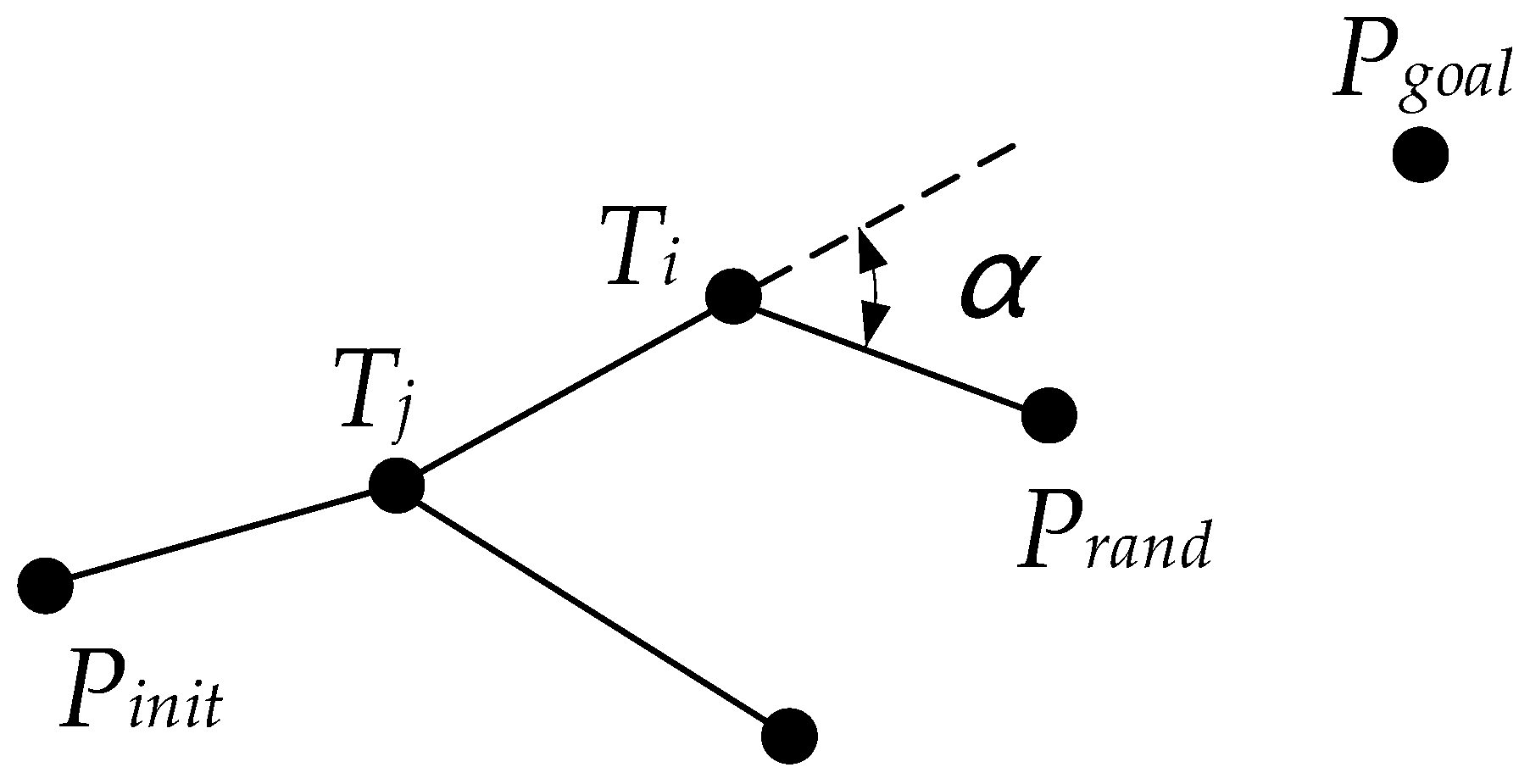
3.2.4. Adaptive Node Extension Strategy

The RRT algorithm will extend the selected node $P_{near}$ to the sampling state $P_{rand}$ when the nearest tree node $P_{near}$ is determined. Due to the adoption of a fixed step size, the random tree either easily leads to collision with obstacles or is slow to converge, resulting in low flexibility and low security. To solve this problem, an adaptive step strategy is designed to use a smaller step when the distance between the nearest tree node $P_{near}$ and the obstacle gets smaller to slow down the growth of the random tree and make the path search more detailed and secure. On the contrary, the step size increases when the distance between the nearest tree node $P_{near}$ and the obstacle increases to improve the growth efficiency of the random tree. Meanwhile, the step size has a minimum threshold to ensure the most basic expansion. Equation (22) shows how to calculate the adaptive step size $L$.

$$L=\{\begin{array}{l}L\max D_l\le D_s\\ L_{\max }\cdot \frac{D_l}{D_s} \frac{D_s}{2}<D_l<D_s\\ \frac{L_{\max }}{2} D_l\le \frac{D_s}{2}\end{array}$$

(22)

where $L_{\max }$ is the maximum fixed step, $D_l$ is the distance between the nearest tree node $P_{near}$ and the obstacle point $P_{obstacle}$.

The random tree reduces several invalid calculations based on the adaptive step size strategy when extending, which can accelerate the running speed of the algorithm, improve the efficiency of the search, and improve the stability of the algorithm.

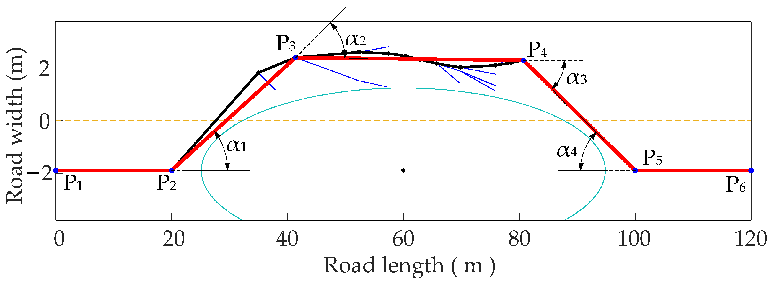
3.2.5. Post-Processing Strategy

After the random tree has grown, the next step is to find and optimize the initial path. Because of the random sampling of the RRT algorithm, the initial path is very tortuous and extremely unsmooth, with many unnecessary turning points, resulting in the condition that the autonomous vehicle has severe mechanical wear when tracking. Therefore, an efficient post-processing strategy is required.

Algorithm 5 outlines the working of the post-processing strategy. It consists of path getting, path pruning, and path smoothing. Path pruning is used to process the initial path to remove unnecessary nodes based on the maximum curvature constraints. Then, the remaining nodes are smoothed by the cubic B-spline curve interpolation.

Algorithm 5: Adaptive Improved RRT POST_PROCESSING ( )

$1. \mathrm{Var} {\mathrm{Q}}_0$$,Q_1$$,Q_2$$,Q_3$$,Q_4$: path

$2. {\mathrm{Q}}_0$$({\mathrm{q}}_{\mathrm{n}}$$\dots ,{\mathrm{q}}_2$$,{\mathrm{q}}_1$$,{\mathrm{q}}_0$)←GET_PATH (T)

$3. {\mathrm{q}}_{\mathrm{root}}$←${\mathrm{q}}_0$$; {\mathrm{q}}_{\mathrm{temp}}$←${\mathrm{q}}_1$;

$4. {\mathrm{Q}}_1$←$({\mathrm{q}}_{\mathrm{root}}$$,{\mathrm{q}}_{\mathrm{temp}}$)

$5. Q_2$←$({\mathrm{q}}_{\mathrm{n}}$$\dots ,{\mathrm{q}}_2$)

$6. \mathrm{While} {\mathrm{q}}_{\mathrm{temp}}$$!={\mathrm{q}}_{\mathrm{n}-1}$ do

$7. {\mathrm{Q}}_3$←$({\mathrm{q}}_{\mathrm{temp}}$$,{\mathrm{q}}_{\mathrm{root}}$$);Q_4$←$({\mathrm{q}}_{\mathrm{root}}$$,{\mathrm{q}}_{\mathrm{temp}}$)

$8. \mathrm{for} \mathrm{each} \mathrm{node} {\mathrm{q}}_{\mathrm{i}}$∈${\mathrm{Q}}_2$

$9. \mathrm{if} \mathrm{Collision}\_\mathrm{Free} ({\mathrm{q}}_{\mathrm{temp}}$$,{\mathrm{q}}_{\mathrm{i}}$)

$10. {\mathrm{Q}}_3$$.\mathrm{Forward}\_\mathrm{Add}\_\mathrm{Node} ({\mathrm{q}}_{\mathrm{i}}$);

11.                          else

$12. {\mathrm{Q}}_3$$.\mathrm{Forward}\_\mathrm{Add}\_\mathrm{Node} ({\mathrm{q}}_{\mathrm{i}}$); break

13.                          end if

14.                      end for

$15. \mathrm{for} \mathrm{each} \mathrm{node} {\mathrm{q}}_{\mathrm{k}}$∈${\mathrm{Q}}_3$$\mathrm{and} {\mathrm{q}}_{\mathrm{k}-1}$∈${\mathrm{Q}}_3$

$16. {\mathrm{q}}_{\mathrm{dou}\_\mathrm{head}}$←${\mathrm{q}}_{\mathrm{k}}$$; {\mathrm{q}}_{\mathrm{head}}$←${\mathrm{q}}_{\mathrm{k}-1}$;

$17. \mathrm{if} (\pi -\mathrm{Angle}(\overrightarrow{{\mathrm{q}}_{\mathrm{temp}}{\mathrm{q}}_{\mathrm{root}}},\overrightarrow{{\mathrm{q}}_{\mathrm{temp}}{\mathrm{q}}_{\mathrm{head}}}))<\beta$

$\mathrm{and} (\pi -\mathrm{Angle}(\overrightarrow{{\mathrm{q}}_{\mathrm{head}}{\mathrm{q}}_{\mathrm{temp}}},\overrightarrow{{\mathrm{q}}_{\mathrm{head}}{\mathrm{q}}_{\mathrm{dou}\_\mathrm{head}}}\left)\right)<\beta$

$18. { \mathrm{Q}}_4$$.\mathrm{Backward}\_\mathrm{Add}\_\mathrm{Node} ({\mathrm{q}}_{\mathrm{k}-1}$);

$19. {\mathrm{q}}_{\mathrm{root}}$←${\mathrm{q}}_{\mathrm{temp}}$$; {\mathrm{q}}_{\mathrm{temp}}$←${\mathrm{q}}_{\mathrm{head}}$; a←k; break

20.                             end if

21.                      end for

$22. {\mathrm{Q}}_1$←${\mathrm{Q}}_1\cup {\mathrm{Q}}_4$

$23. {\mathrm{Q}}_2$←$({\mathrm{q}}_{\mathrm{n}}$$\dots , {\mathrm{q}}_{\mathrm{a}}$)

24. endWhile

$25. {\mathrm{Q}}_1$$.\mathrm{Backward}\_\mathrm{Add}\_\mathrm{Node} ({\mathrm{q}}_{\mathrm{n}}$)

26. trajectory←$\mathrm{Cubic}\_\mathrm{Bspline} ({\mathrm{Q}}_1$)

Path Pruning

Lines 3–25 in Algorithm 5 are the path pruning part of the post-processing strategy. A set ${\mathrm{Q}}_0$ of nodes of the valid path from the forward point of the target point to the parent point of the starting point is obtained by reversely searching the random tree utilizing the function $\mathrm{GET}\_\mathrm{PATH} ( )$.

Based on the set ${\mathrm{Q}}_0$, the first path point, the parent node of the starting point, is defined as the root point ${\mathrm{q}}_{\mathrm{root}}$, and the second path point, namely the starting point, is defined as the current point ${\mathrm{q}}_{\mathrm{temp}}$$.$ Afterward, we connect that current point and the first subsequent path point with a line segment and then continue to connect that current point and one of all subsequent path points with a line segment successively in sequence until there is an intersection between the line segment and the obstacle space. In this case, the parent node of the collision point, that is, the path point resulting in the intersection is defined as the forward point ${\mathrm{q}}_{\mathrm{head}}$, and the collision point is defined as the double-forward point ${\mathrm{q}}_{\mathrm{dou}\_\mathrm{head}}$$.$ Meanwhile, the included angle between the line between the forward point ${\mathrm{q}}_{\mathrm{head}}$ and the current point ${\mathrm{q}}_{\mathrm{temp}}$ and the line between the current point ${\mathrm{q}}_{\mathrm{temp}}$ and the root point ${\mathrm{q}}_{\mathrm{root}}$, and the included angle between the line between the forward point ${\mathrm{q}}_{\mathrm{head}}$ and the current point ${\mathrm{q}}_{\mathrm{temp}}$ and the line between the forward point ${\mathrm{q}}_{\mathrm{head}}$ and the double-forward point ${\mathrm{q}}_{\mathrm{dou}\_\mathrm{head}}$ are calculated. When they all are less than the steering angle of the wheel $\beta$, the current point ${\mathrm{q}}_{\mathrm{temp}}$ is defined as the new root point ${\mathrm{q}}_{\mathrm{root}}$, and the forward point ${\mathrm{q}}_{\mathrm{head}}$ is defined as the new current point ${\mathrm{q}}_{\mathrm{temp}}$$.$ On the contrary, we continue to make the parent node of the forward point ${\mathrm{q}}_{\mathrm{head}}$ be defined as the forward point ${\mathrm{q}}_{\mathrm{head}}$ and make the forward point ${\mathrm{q}}_{\mathrm{head}}$ be defined as the double-forward point ${\mathrm{q}}_{\mathrm{dou}\_\mathrm{head}}$ successively in sequence, and continually calculate the included angle between the line between the forward point ${\mathrm{q}}_{\mathrm{head}}$ and the current point ${\mathrm{q}}_{\mathrm{temp}}$ and the line between the current point ${\mathrm{q}}_{\mathrm{temp}}$ and the root point ${\mathrm{q}}_{\mathrm{root}}$, and the included angle between the line between the forward point ${\mathrm{q}}_{\mathrm{head}}$ and the current point ${\mathrm{q}}_{\mathrm{temp}}$ and the line between the forward point ${\mathrm{q}}_{\mathrm{head}}$ and the double-forward point ${\mathrm{q}}_{\mathrm{dou}\_\mathrm{head}}$ until those angles are less than the steering angle of the wheel $\beta$. Thus, the current point ${\mathrm{q}}_{\mathrm{temp}}$ and the forward point ${\mathrm{q}}_{\mathrm{head}}$ are defined as both a new root point ${\mathrm{q}}_{\mathrm{root}}$ and a new current point ${\mathrm{q}}_{\mathrm{temp}}$. Then, the preceding operations are performed on subsequent path points until the goal point is found. Such path pruning can minimize the number of line segments forming the initial path and reduce unnecessary costs in the distance of the path under the condition of meeting the requirement of the included angle between path points. Specifically, as shown in Figure 7, the black polyline is the initial path obtained by the reverse search. Because the connecting lines between the blue nodes P₁, P₂, P₃, P₄, P₅, and P₆ do not intersect with the expanded safe ellipse, these nodes can be connected directly by line segments to delete the redundant nodes between them and have no sharp angles between those line segments, thus obtaining a relatively gentle path sequence. In addition, the included angles of the connecting lines between these nodes are less than $\beta$; that is, α₁, α₂, α₃, and α₄ are less than $\beta$.

Cubic B-Spline Smoothing Method

Because the curvature of the path processed by path pruning is not continuous, it is essential to optimize the path to make the vehicle drive steadily and safely. The B-spline can make local adjustments to the path without changing the entire shape of the path when smoothing and make the generated path have the advantages of continuous curvature, and so on, which makes it widely used in motion planning [34,35,36]. Therefore, the cubic B-spline is used to interpolate and fit the path points obtained by the path pruning to achieve the purpose of path smoothing. Equation (23) shows how to calculate the cubic B-spline curve.

$$C\left(u\right)={\displaystyle {\sum }_{i=0}^n{P}_i\cdot N_{i,4}\left(u\right),}u\in \left[0,1\right)$$

(23)

where $N_{i,4}\left(u\right)$ is the basic function of the cubic B-spline curve, corresponding to the control point $P_i$. It can be obtained using Cox–de Boor recursion. Equations (24) and (25) show how to calculate the basic function of the cubic B-spline curve.

$$N_{i,0}\left(u\right)=\{\begin{array}{l}1 u_i\le u\le u_{i+1}\\ 0 \mathrm{otherwise}\end{array}$$

(24)

$$N_{i,4}\left(u\right)=\frac{u-u_i}{u_{i+4}-u_i}{N}_{i,4-1}\left(u\right)+\frac{u_{i+4+1}-u}{u_{i+4+i}-u_{i+1}}{N}_{i+1,4-1}\left(u\right)$$

(25)

For making the curve tangent to the first and last sides of the path generated by the path pruning and passing through the first and last path points, the node vector of the cubic B-spline can be set to keep the nodes at both ends having four times repetition.

The length of the generated path is shortened to the maximum extent, and some unnecessary back and forth steering belonging to this path is removed after using the post-processing strategy. Meanwhile, this path can meet the vehicle steering constraints.

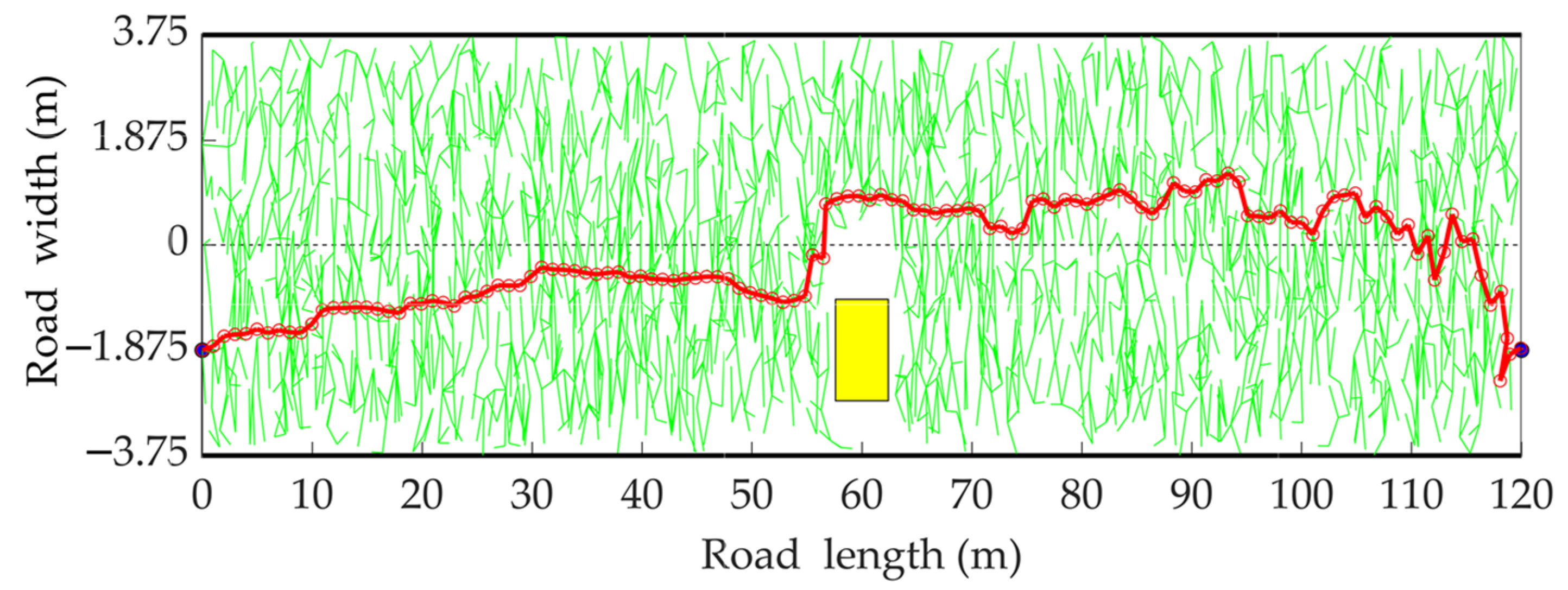
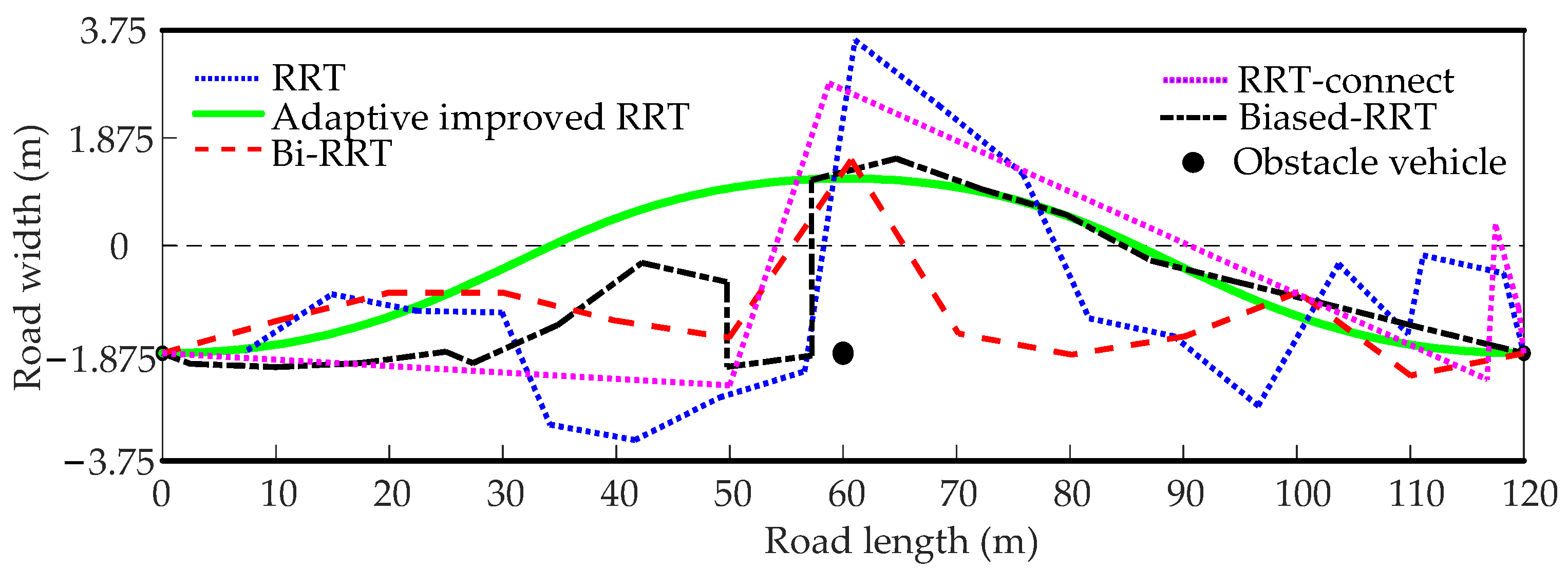
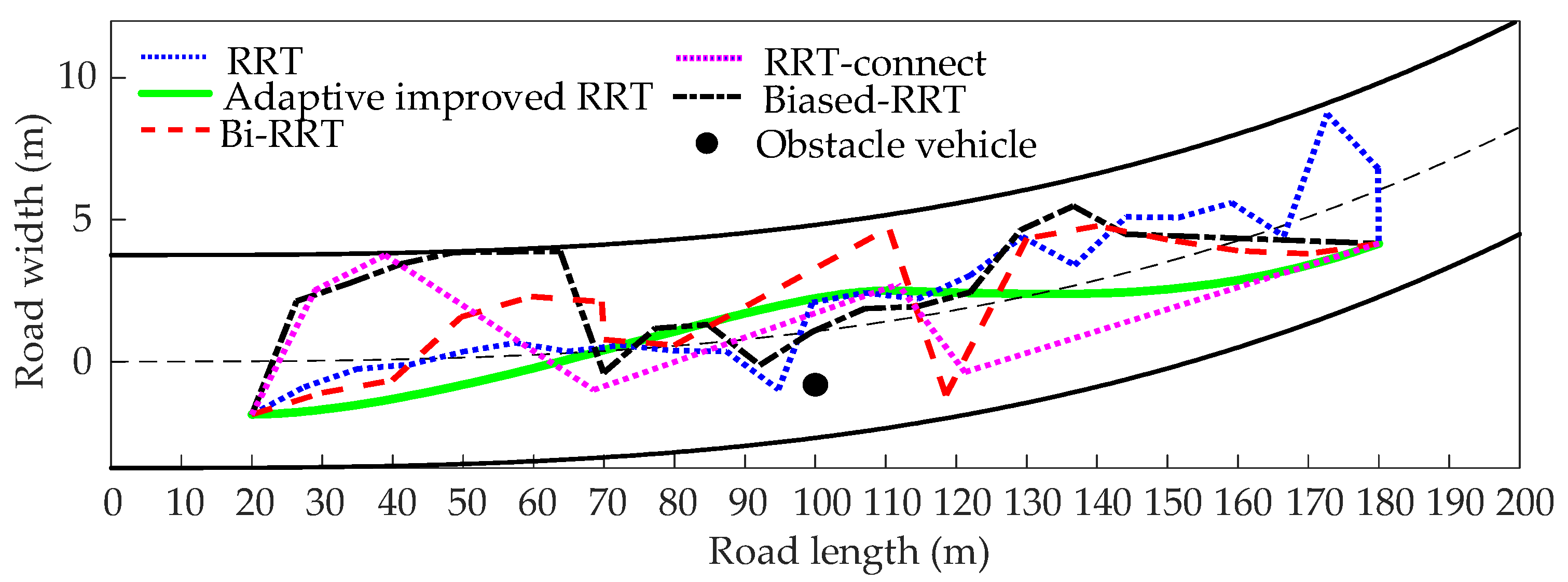
4. Simulation Experiments

In this section, we verify the performance of the adaptive improved RRT algorithm through simulation experiments for the convenience of expression. The simulation experiments are divided into two parts. In the first part, we verify the correctness and superiority of this algorithm in certain lane environments by comparing it with basic RRT, bidirectional RRT, biased RRT, and RRT-connect. In the second part, the road environments are simulated in CarSim. Then, an appropriate vehicle model and driver model selected in the model database of CarSim are used to simulate the driving process of the actual vehicle to verify the effectiveness and practicability of this algorithm.

4.1. Performance Comparison of Several RRT Algorithms

To compare the performance of the adaptive improved RRT algorithm with other algorithms, we constructed two road scenarios, in which the host vehicle is represented in blue, the obstacle vehicle is represented in yellow, the lane borders are represented in solid black curves, and the road center line is represented in a dashed orange curve. Figure 8a shows the straight road environment, and Figure 8b shows the curved road environment. All parameters in the whole simulation process are shown in

Table 1. Road parameters.

Road Type	Road Length (m)	Single Lane Width (m)	Initial Point	Target Point	Obstacle Point
Straight	120	3.75	0, −1.875	120, −1.875	60, −1.875
Curve	200	3.75	20, −1.865	180, 4.160	100, −0.813

and

Table 2. Other parameters. Contrast step size ∆L (m).

Parameter	Value	Parameter	Value
Obstacle vehicle width $\mathrm{W}$ (m)	1.8	Terminal step size δ (m)	20
Obstacle vehicle length $\mathrm{L}$ (m)	4.8	Constraint angle $\phi$ (°)	30
Expansion coefficient $s$	$\sqrt{3}$	Weighted coefficient ${\omega }_1$	0.5
Friction coefficient $\mu$	0.8	Weighted coefficient $m_1$	0.5
Acceleration of gravity $\mathrm{g}$ (m/s2)	9.8	Weighted coefficient $m_2$	0.5
Host vehicle speed $\mathrm{V}$ (km/h)	60	Weighted coefficient $n_1$	0.7
Biased probability ${\rho }_{goal}$	0.1	Weighted coefficient $n_2$	0.3
Maximum step size $L_{max}$ (m)	20

.

For describing the performance of the algorithm more objectively, the definition of benchmarking parameters to describe the simulation results of the algorithm quantitatively is as follows:

Node: The number of nodes in the constructed graph.

Length: The length of the generated path.

Segment: the number of line segments that make up the generated path. The adaptive improved RRT algorithm specifically refers to the number of line segments of the path before the smoothing process.

Time: The amount of time spent on the planning process in seconds.

Thirty simulations were performed on each algorithm to offset the random deviation of a single test.

Table 3. Comparison of several RRT algorithms in the straight road environment: mean values in 30 runs.

Algorithm	Node	Length	Segment	Time
Basic	37.47	124.435	15.7	0.026
Biased	25.77	122.746	11.57	0.017
Bi	14.90	122.105	10.03	0.016
Connect	10.50	124.378	4.43	0.011
Adaptive-Improved	22.50	120.290	5.23	0.024

and

Table 4. Comparison of several RRT algorithms in the curved road environment: mean values in 30 runs.

Algorithm	Node	Length	Segment	Time
Basic	26.93	162.634	16.57	1.755
Biased	21.13	161.884	14.10	1.411
Bi	14.00	161.032	12.13	0.386
Connect	4.87	162.243	3.30	0.299
Adaptive-Improved	26.37	160.141	4.23	3.257

, respectively, showed the average number of nodes, path length, segments, and running time of those algorithms in straight and curved road environments. Compared with the biased RRT, the bidirectional RRT, and the RRT-connect, the planning time and the path length of the basic RRT were the largest, and those of the other three algorithms were reduced to a certain extent, which was because the biased RRT increased the number of the goal point as the sampling point in the sampling process, the bidirectional RRT explored feasible space through the simultaneous growth of two trees, and the RRT-connect added the greedy method to the growth process of the two trees. The path length of the RRT-connect was more than that of the bidirectional RRT, which indicated that the greedy method might extend trees regardless of goodness in that direction, causing a negative optimization of the path length. As for the adaptive improved RRT algorithm, the number of tree nodes and path segments was relatively minimal compared with the basic RRT and the biased RRT, especially in path segments, but was relatively larger than the RRT-connect when considering the feasibility of the path. Compared with the bidirectional RRT, the number of tree nodes of the adaptive improved RRT algorithm was more significant, but the number of the path segments was relatively small. The main reason is that the adaptive improved RRT algorithm is based on the framework of the basic RRT and takes path pruning into account. The smaller number of path segments of the adaptive improved RRT algorithm can reduce the control points to facilitate smoothing and decrease the difficulty of autonomous driving. For the average planning time, the performance of the adaptive improved algorithm was superior to that of the basic RRT and was under that of the biased RRT, the bidirectional RRT, and RRT-connect, in the straight road environment. When applied to the curved road environment, the adaptive improved algorithm needed to take more time to plan the path than other algorithms did. However, compared with the other four algorithms, the path length generated by the adaptive improved RRT was minimal, mainly due to a series of novel heuristics, including adaptive directed sampling, reasonable node selection, and path pruning. In general, the adaptive improved RRT algorithm greatly improved the quality of the path, but it needed to appropriately sacrifice the planning time when applied to the curved road environment.

Figure 9 and Figure 10 showed the paths planned by the algorithms in the straight road environment and the curved road environment, respectively. The blue dotted curve, the red dashed curve, the black dash-dotted curve, the purple dotted curve, and the solid green curve were the paths planned by the basic RRT, the bidirectional RRT, the biased RRT, the RRT-connect, and the adaptive improved RRT, respectively. From those, we could see that the paths generated by the basic RRT, the bidirectional RRT, the biased RRT, and RRT-connect were broken lines, including too many unnecessary and irregular steering corners, and their curvatures changed significantly and were discontinuous, which indicated that these paths did not satisfy the steering requirements of autonomous driving. The path generated by the adaptive improved RRT was desirable, the smoothest without the unnecessary detour, and the trend of its extension was natural, resulting in it being very easy to track this path for the autonomous vehicle. At the same time, we could see that the paths generated by the basic RRT, the bidirectional RRT, the biased RRT, and RRT-connect, respectively, were always starting to avoid a collision when close to the obstacle. On the contrary, the path generated by the adaptive improved RRT started to avoid a collision at a safe distance from the obstacle, which was vital for safe driving, and the safe distance could be automatically adjusted depending on the host vehicle’s speed.

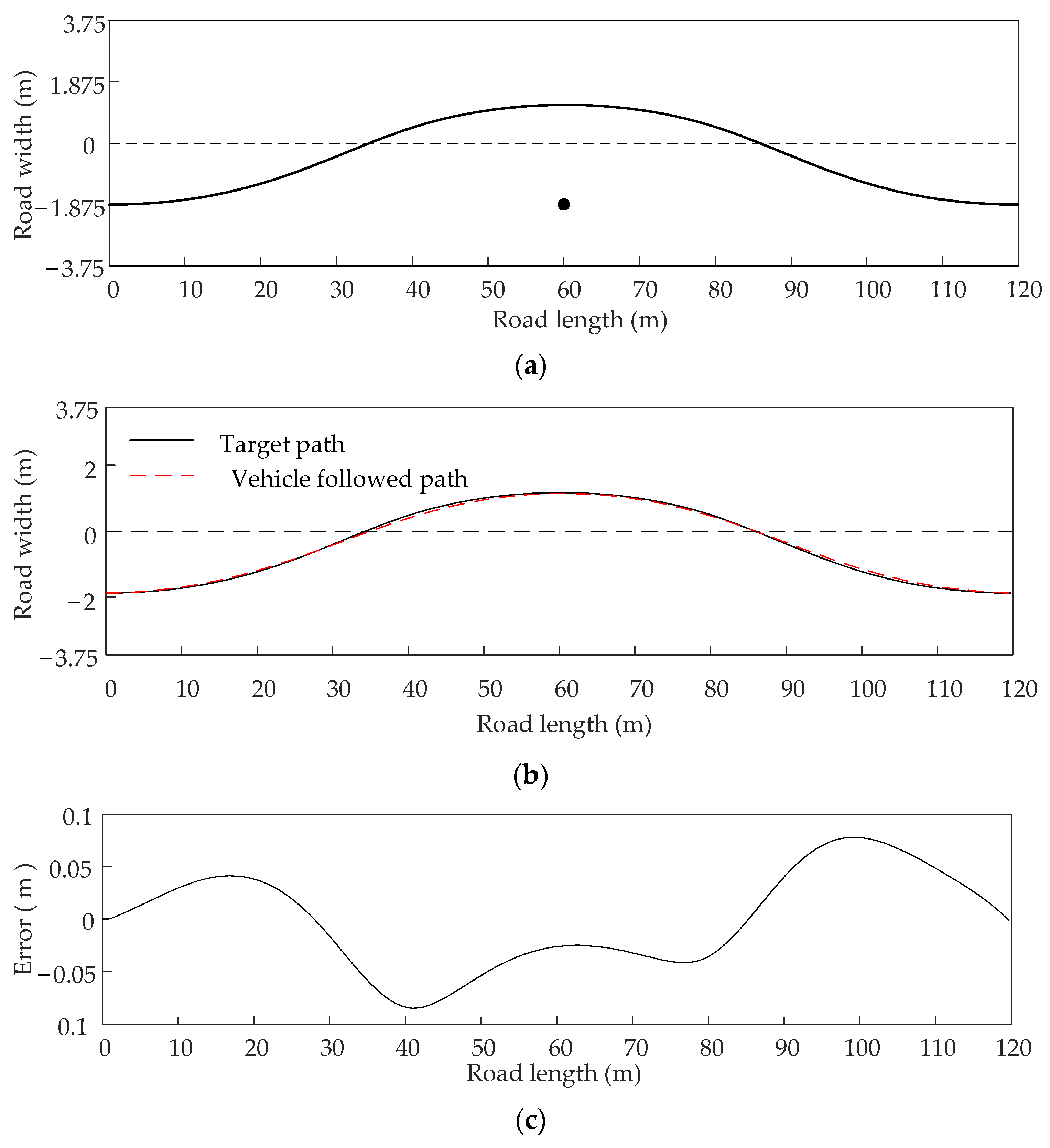
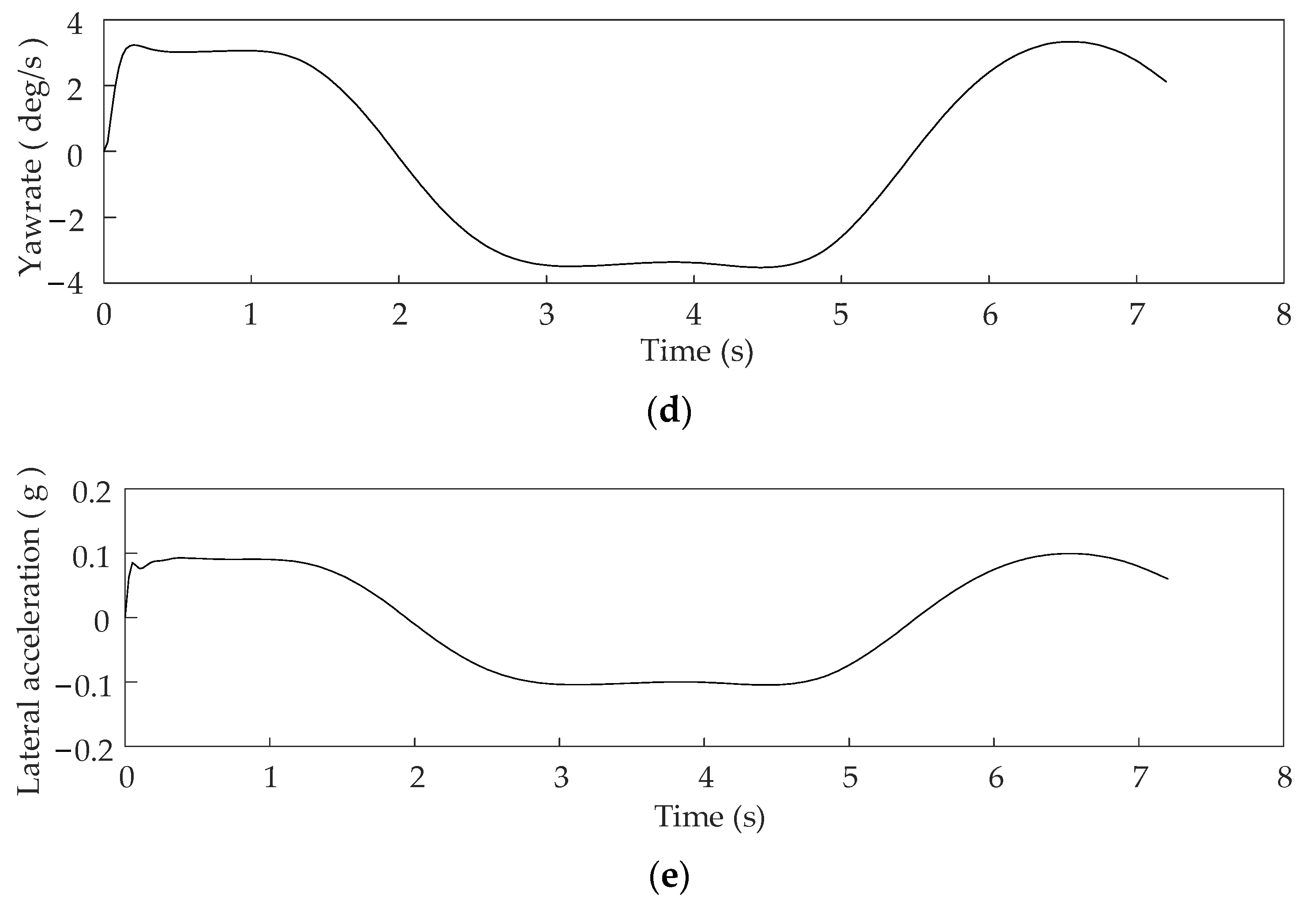
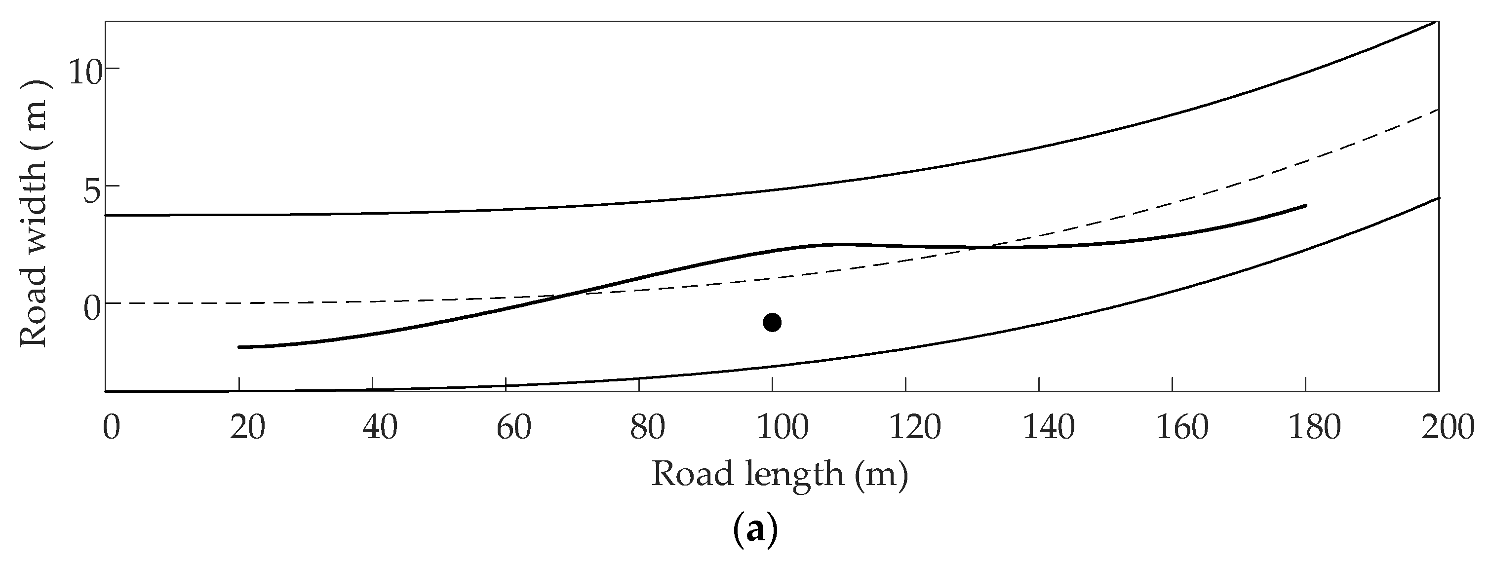
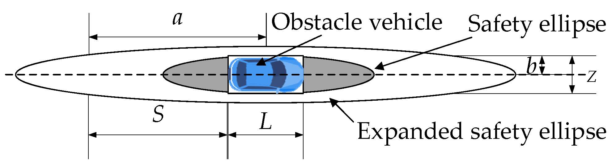
4.2. Path Following Validation

In order to evaluate the effectiveness and practicality of the adaptive improved RRT algorithm, it is necessary to follow the planned path by an autonomous vehicle. Once the path generation process was completed, the path-following experiment was simulated in CarSim. When the host vehicle follows the path, its yaw velocity and lateral acceleration can be obtained as dynamic performance indicators for monitoring the stability of the path. The followed path is represented in the red dashed line, and the target path is represented in the solid black line.

We considered the straight road scenario described in Figure 8a; namely, the host vehicle moved at a constant speed of 60 km/h in the middle of the right lane, and the obstacle vehicle was in front of the host vehicle along this lane. The result that the host vehicle could successfully avoid the collision with the obstacle vehicle is shown in Figure 11a. The target path and the followed path are shown in Figure 11b. The following error between the followed path and the target path was within 0.1 m, as shown in Figure 11c, and it was small and quite satisfactory. The yaw velocity of the host vehicle was within 4 deg/s, and its lateral acceleration was within the range of 0.15 g, respectively shown in Figure 11d,e. Therefore, the host vehicle could remain stable in the simulation, and the trajectory could be considered acceptable.

This local path planning could also deal with the curved road scenario, as shown in Figure 8b. We used the method described in the construction of the road environment to build a curved road environment. The initial curvature of the road was equal to 0, and the final curvature of the road was equal to 0.0012 within a horizontal distance of 200 m. The host vehicle moved in the right lane at a constant speed of 60 km/h, and the obstacle vehicle was also in front of the host vehicle along this lane. The result of the planning is shown in Figure 12a; the host vehicle could avoid collision with the obstacle vehicle in front of it on the curved road successfully. The followed path and the target path are shown in Figure 12b. The following error between the followed path and the target path was within the range of 0.1 m and was small, as shown in Figure 12c. The yaw velocity of the host vehicle was within 4 deg/s, and its lateral acceleration was within 0.15 g, respectively, as shown in Figure 12d,e. Therefore, the given trajectory was also considered to be feasible.

5. Conclusions

In this paper, with the aim of remedying the deficiencies of the basic RRT algorithm in the quality of the planning path in certain lane environments, the adaptive improved RRT algorithm is proposed to solve the local path planning problem of autonomous vehicles. This algorithm adopts the adaptive directed sampling strategy, making the random tree grow toward a direction near the reference trajectory line and the target point and avoiding unnecessary sampling in an already sampled space to improve sampling efficiency. It uses the reasonable node selection strategy to make the random tree grow more directionally, improving the length and the smoothness of the path to a certain extent. Meanwhile, the adaptive node expansion strategy is introduced to make the expansion of nodes change with the distance from the obstacle, improving the success rate of extension. The amplified constraint is used to ensure that the generated path can avoid the obstacle in advance at a safe distance. The post-processing strategy is employed to improve the quality of the path, making the generated path obtain the shortest length and meet the steering requirements. Simulation results show that the adaptive improved RRT algorithm is successful and feasible in local path planning and can plan a high-quality path in a certain lane environment. The proposed algorithm is instructive for the global path planning of autonomous vehicles in structured road environments and provides a test sample for the tracking control method developed in the subsequent research. Meanwhile, it can also apply to the local path planning of wheeled robots.

From the perspective of the future development of the autonomous vehicle, the algorithm proposed by this paper still has limitations needing to be overcome. The planning time is not very satisfactory, especially when planning a path in the curved road environment, and no actual on-site experiment was carried out to test the performance of the improved algorithm in practice. In our future proceedings, a parallel calculation will be integrated to speed up the running of the algorithm, further reducing the planning time. In addition, we will implement the actual on-site experiment to test the gap between the simulated and actual performance of the improved algorithm after the preparation of other modules, including environmental perception, tracking control, and vehicle platform.

References

1. Malik, S.; Khattak, H.A.; Ameer, Z.; Shoaib, U.; Rauf, H.T.; Song, H. Proactive Scheduling and Resource Management for Connected Autonomous Vehicles: A Data Science Perspective. IEEE Sens. J. 2021, 21, 25151–25160. [Google Scholar] [CrossRef]
2. Claussmann, L.; Revilloud, M.; Gruyer, D.; Glaser, S. A Review of Motion Planning for Highway Autonomous Driving. IEEE Trans. Intell. Transp. Syst. 2020, 21, 1826–1848. [Google Scholar] [CrossRef] [Green Version]
3. Hang, P.; Chen, X.B. Towards Autonomous Driving: Review and Perspectives on Configuration and Control of Four-Wheel Independent Drive/Steering Electric Vehicles. Actuators 2021, 10, 184. [Google Scholar] [CrossRef]
4. Hnewa, M.; Radha, H. Object Detection Under Rainy Conditions for Autonomous Vehicles: A Review of State-of-the-Art and Emerging Techniques. IEEE Signal Process. Mag. 2021, 38, 53–67. [Google Scholar] [CrossRef]
5. Kim, K.; Kim, J.S.; Jeong, S.; Park, J.H.; Kim, H.K. Cybersecurity for autonomous vehicles: Review of attacks and defense. Comput. Secur. 2021, 103, 27. [Google Scholar] [CrossRef]
6. Li, X.C.; Zhu, S.; Aksun-Guvenc, B.; Guvenc, L. Development and Evaluation of Path and Speed Profile Planning and Tracking Control for an Autonomous Shuttle Using a Realistic, Virtual Simulation Environment. J. Intell. Robot. Syst. 2021, 101, 23. [Google Scholar] [CrossRef]
7. Kim, J.; Jo, K.; Chu, K.; Sunwoo, M. Road-model-based and graph-structure-based hierarchical path-planning approach for autonomous vehicles. Proc. Inst. Mech. Eng. Part D-J. Automob. Eng. 2014, 228, 909–928. [Google Scholar] [CrossRef]
8. Khatib, O. Real-time obstacle avoidance for manipulators and mobile robots. In Proceedings of the 1985 IEEE International Conference on Robotics and Automation, St. Louis, MO, USA, 25–28 March 1985; Volume 2, pp. 500–505. [Google Scholar]
9. Qi, B.K.; Li, M.; Yang, Y.; Wang, X.Y. Research on UAV path planning obstacle avoidance algorithm based on improved artificial potential field method. 2nd International Conference on Internet of Things. In Proceedings of the Artificial Intelligence and Mechanical Automation, Hangzhou, China, 14–16 May 2021; Volume 1948, p. 012060. [Google Scholar]
10. Huang, Y.; Ding, H.; Zhang, Y.; Wang, H.; Cao, D.; Xu, N.; Hu, C.A. Motion Planning and Tracking Framework for Autonomous Vehicles Based on Artificial Potential Field-Elaborated Resistance Network Approach. IEEE Trans. Ind. Electron. 2020, 67, 1376–1386. [Google Scholar] [CrossRef]
11. Sang, H.; You, Y.; Sun, X.; Zhou, Y.; Liu, F. The hybrid path planning algorithm based on improved A* and artificial potential field for unmanned surface vehicle formations. Ocean. Eng. 2021, 223, 108709. [Google Scholar] [CrossRef]
12. Song, X.L.; Cao, H.T.; Huang, J. Vehicle path planning in various driving situations based on the elastic band theory for highway collision avoidance. Proc. Inst. Mech. Eng. Part D-J. Automob. Eng. 2013, 227, 1706–1722. [Google Scholar] [CrossRef]
13. Zhang, H.M.; Li, M.L. Rapid path planning algorithm for mobile robot in dynamic environment. Adv. Mech. Eng. 2017, 9, 12. [Google Scholar] [CrossRef]
14. Liu, L.S.; Lin, J.F.; Yao, J.X.; He, D.W.; Zheng, J.S.; Huang, J.; Shi, P. Path Planning for Smart Car Based on Dijkstra Algorithm and Dynamic Window Approach. Wirel. Commun. Mob. Comput. 2021, 2021, 12. [Google Scholar] [CrossRef]
15. Zhang, L.; Li, Y. Mobile Robot Path Planning Algorithm Based on Improved a Star. In Proceedings of the 4th International Conference on Advanced Algorithms and Control Engineering, Sanya, China, 29–31 January 2021; Volume 1848, p. 012013. [Google Scholar]
16. Desaraju, V.R.; How, J.P. Decentralized path planning for multiple agents in complex environments using rapidly-exploring random trees. In Proceedings of the IEEE International Conference on Robotics & Automation, Shanghai, China, 9–13 May 2011; pp. 4956–4961. [Google Scholar]
17. Palmieri, L.; Kai, O.A. Distance metric learning for RRT-based motion planning with constant-time inference. In Proceedings of the IEEE International Conference on Robotics and Automation, Seattle, WA, USA, 26–30 May 2015; pp. 637–643. [Google Scholar]
18. Jaillet, L.; Cortés, J.; Siméon, T. Sampling-Based Path Planning on Configuration-Space Costmaps. IEEE Trans. Robot 2010, 26, 635–646. [Google Scholar] [CrossRef] [Green Version]
19. Liu, H.Y.; Zhang, X.B.; Wen, J.; Wang, R.H.; Chen, X. Goal-biased Bidirectional RRT based on Curve-smoothing. In Proceedings of the 5th IFAC Symposium on Telematics Applications, Chengdu, China, 25–27 September 2019; Volume 52, pp. 255–260. [Google Scholar]
20. Meng, L.; Song, Q.; Zhao, Q.J. UAV path re-planning based on improved bidirectional RRT algorithm in dynamic environment. In Proceedings of the 3rd IEEE International Conference on Control, Automation and Robotics, Nagoya, Japan, 22–24 April 2017; pp. 658–661. [Google Scholar]
21. Wei, K.; Ren, B. A Method on Dynamic Path Planning for Robotic Manipulator Autonomous Obstacle Avoidance Based on an Improved RRT Algorithm. Sensors 2018, 18, 571. [Google Scholar] [CrossRef] [Green Version]
22. Yang, K. Anytime synchronized-biased-greedy rapidly-exploring random tree path planning in two dimensional complex environments. Int. J. Control Autom. Syst. 2011, 9, 750–758. [Google Scholar] [CrossRef]
23. Chen, L.; Shan, Y.; Tian, W.; Li, B.; Cao, D. A Fast and Efficient Double-Tree RRT* Like Sampling-Based Planner Applying on Mobile Robotic Systems. IEEE/ASME Trans. Mechatron. 2018, 24, 2568–2578. [Google Scholar] [CrossRef]
24. Kang, J.G.; Lim, D.W.; Choi, Y.S.; Jang, W.J.; Jung, J.W. Improved RRT-Connect Algorithm Based on Triangular Inequality for Robot Path Planning. Sensors 2021, 21, 333. [Google Scholar] [CrossRef]
25. Lee, H.; Kim, H.; Kim, H.J. Planning and Control for Collision-Free Cooperative Aerial Transportation. IEEE Trans. Autom. Sci. Eng. 2018, 15, 189–201. [Google Scholar] [CrossRef]
26. Rodriguez, S.; Tang, X.; Lien, J.M.; Amato, N.M. An obstacle-based rapidly-exploring random tree. In Proceedings of the IEEE International Conference on Robotics and Automation, Orlando, FL, USA, 15–19 May 2006; pp. 895–900. [Google Scholar]
27. Gan, Y.; Zhang, B.; Ke, C.; Zhu, X.; He, W.; Ihara, T. Research on Robot Motion Planning Based on RRT Algorithm with Nonholonomic Constraints. Neural Process. Lett. 2021, 53, 3011–3029. [Google Scholar] [CrossRef]
28. Chen, J.G.; Zhao, Y.; Xu, X. Improved RRT-Connect Based Path Planning Algorithm for Mobile Robots. IEEE Access. 2021, 9, 145988–145999. [Google Scholar] [CrossRef]
29. Ge, Q.; Li, A.; Li, S.; Du, H.; Huang, X.; Niu, C. Improved Bidirectional RRT * Path Planning Method for Smart Vehicle. Math. Probl. Eng. 2021, 2021, 6669728. [Google Scholar] [CrossRef]
30. Kuwata, Y.; Teo, J.; Fiore, G.; Karaman, S.; Frazzoli, E.; How, J.P. Real-time motion planning with applications to autonomous urban driving. IEEE Trans. Control Syst. Technol. 2009, 17, 1105–1118. [Google Scholar] [CrossRef]
31. Lau, B.; Sprunk, C.; Burgard, W. Kinodynamic motion planning for mobile robots using splines. In Proceedings of the IEEE RSJ International Conference on Intelligent Robots and Systems, St Louis, MO, USA, 10–15 October 2009; pp. 2427–2433. [Google Scholar]
32. Thanh, P.H.; Nguyen, V.H.; Konigorski, U. A Time-optimal Trajectory Generation Approach with Non-uniform B-splines. Int. J. Control Autom. Syst. 2021, 19, 3947–3955. [Google Scholar]
33. Pappas, G.J.; Kyriakopoulos, K.J. Stabilization of non-holonomic vehicles under kinematic constraints. Int. J. Control 1995, 61, 933–947. [Google Scholar] [CrossRef]
34. Rodrigues, R.T.; Aguiar, A.P.; Pascoal, A. A coverage planner for AUVs using B-splines. In Proceedings of the IEEE/OES Autonomous Underwater Vehicle Workshop (AUV), Porto, Portugal, 6–9 November 2018; pp. 1–6. [Google Scholar]
35. Noreen, I. Collision Free Smooth Path for Mobile Robots in Cluttered Environment Using an Economical Clamped Cubic B-Spline. Symmetry 2020, 12, 1567. [Google Scholar] [CrossRef]
36. Elbanhawi, M.; Simic, M.; Jazar, R. Continuous-curvature bounded trajectory planning using parametric splines. In Proceedings of the KES International Conference on Smart Digital Futures, Chania, Greece, 18–20 June 2014; Volume 262, pp. 513–522. [Google Scholar]
Figure 1. Curved road environment.
Actuators 11 00109 g001
Figure 2. Road reference coordinate frame.
Actuators 11 00109 g002
Figure 3. The vehicle kinematic model.
Actuators 11 00109 g003
Figure 4. Performance of the basic RRT for a straight road.
Actuators 11 00109 g004
Figure 5. The obstacle vehicle expansion.
Actuators 11 00109 g005
Figure 6. Nodes of the random tree.
Actuators 11 00109 g006
Figure 7. Path pruning.
Actuators 11 00109 g007
Figure 8. Road environments. (a) Straight road environment. (b) Curved road environment.
Actuators 11 00109 g008
Figure 9. Performance contrast in straight road environment.
Actuators 11 00109 g009
Figure 10. Performance contrast in curved road environment.
Actuators 11 00109 g010
Figure 11. Path tracking results in the straight road environment. (a) Planned path on straight road. (b) Path following result on straight road. (c) Path following error on straight road. (d) Yaw velocity on straight road. (e) Lateral acceleration on straight road.
Actuators 11 00109 g011aActuators 11 00109 g011b
Figure 12. Path tracking results in curved road environment. (a) Planned path on curved road. (b) Path following result on curved road. (c) Path following error on curved road. (d) Yaw velocity on curved road. (e) Lateral acceleration on curved road.
Actuators 11 00109 g012aActuators 11 00109 g012b