Research on an Intelligent Driving Algorithm Based on the Double Super-Resolution Network

Abstract

Semantic segmentation plays a very important role in image processing, and has been widely used in intelligent driving, medicine, and other fields. With the development of semantic segmentation, the model has become more and more complex and the resolution of training pictures is higher and higher, so the requirements for required hardware facilities have become higher and higher. Many high-precision networks are difficult to apply in intelligent driving vehicles with limited hardware conditions, and will bring delay to recognition, which is not allowed in practical application. Based on the Dual Super-Resolution Learning (DSRL) network, this paper proposes a network model for training high-resolution pictures, adding a high-resolution convolution module which improves segmentation accuracy and speed while reducing computation. In a CamVid dataset, taking the road category as an example, IOU is 95.23%, which is 4% higher than DSRL, the real-time segmentation time of the same video is reduced by 46% from 120 s to 65 s, and the segmentation effect is better and faster, which greatly alleviates the recognition delay caused by high-resolution input.

1. Introduction

Semantic segmentation is a basic computer vision task. Its purpose is to classify each pixel in the picture. It is widely used in the fields of intelligent driving, medical imaging, and pose analysis. According to research [1], when traditional cars are replaced by private autonomous vehicles, the number of cars owned by each family can be reduced, the maintenance cost will be less than traditional cars, and the mileage of family vehicles will increase by 57%. According to a survey, consumers are willing to pay the premium related to the purchase of vehicles equipped with automatic equipment. Research [2] shows that cumulative energy and greenhouse gas can be reduced by 60% in the basic case after a series of strategic deployments, and can be further reduced by 87% through accelerated grid decarburization, dynamic performance sharing, vehicle life extension, the improved efficiency of computer systems, the improved fuel efficiency of new vehicles, etc. Therefore, intelligent driving vehicles will be widely used. However, in the field of intelligent driving, semantic segmentation needs to maintain real-time detection while maintaining high accuracy. However, in an application with limited hardware facilities, a high-precision network cannot be put into use, and the recognition delay is also very large. The following are some classic networks for semantic segmentation: UNet [3], Deeplabs [4,5,6], PSPNet [7], SegNet [8], etc. These semantic segmentation networks usually need to use high-resolution atlas training to achieve high accuracy. High-resolution pictures can effectively transfer the features in pictures and facilitate network learning. Therefore, high-resolution features are very important in high-precision networks. At present, there are two main ways to maintain high-resolution performance. One is to use void convolution to maintain high-resolution features, and the other is to combine top-down paths and horizontal connections, such as with UNet. Both methods can effectively prevent feature disappearance due to too much convolution, but these methods themselves consume very many computing resources. On this basis, taking high-resolution images as input will further increase the amount of network computing and image segmentation time. In order to reduce the cost of automatic driving, some studies [9] have improved the hardware by using a fisheye camera instead of a vision and LiDAR odometer system. In recent years, the compressed network used in devices with limited hardware resources has attracted people′s attention, but there is still a certain gap between the prediction accuracy of the current network and the network model trained by high-resolution atlas. In order to reduce the gap between the two networks above, some compressed networks also choose high-resolution pictures as input (for example, 1024 × 2048 or 512 × 1024). In order to reduce the burden on the network when high-resolution pictures are used as input, ESPNets [10,11] have been proposed to accelerate convolution calculation by using split merge or reducing the expand principle. Others use efficient classification networks (such as MobileNet [12] and ShuffleNet [13]) or some compression technologies (such as pruning [14] and vector quantization) to accelerate segmentation, but the effect is not ideal. The existing convolution kernel has two main disadvantages: one is that the receptive field is small and difficult to capture in long-distance dependence; the other is that the information between channels is redundant. On this basis, D Li [15] et al. proposed involution; that is, the convolution kernel is multiplexed in space and independent in the channel, which can be used to accelerate the speed of convolution. Li Wang [16] et al. proposed a dual super-resolution learning network (DSRL): a compressed network for high-resolution atlas training that has a certain improvement compared with the previous methods, but the DSRL network is still poor at detecting the details of objects. Therefore, in this paper, a new network framework is designed based on DSRL to alleviate this problem. More specifically, the network in this paper consists of two parts: one part is the super-resolution network, and the other is the high-resolution picture convolution network. The internal convolution is used to replace the partial convolution, which not only reduces the network parameters, but also improves the segmentation accuracy.

2. Materials and Methods

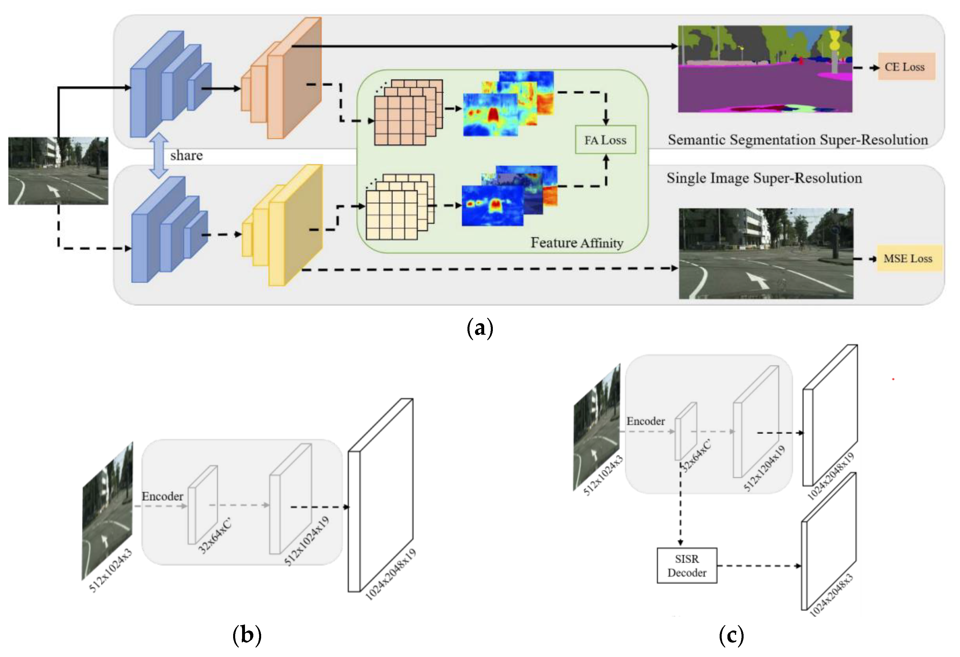
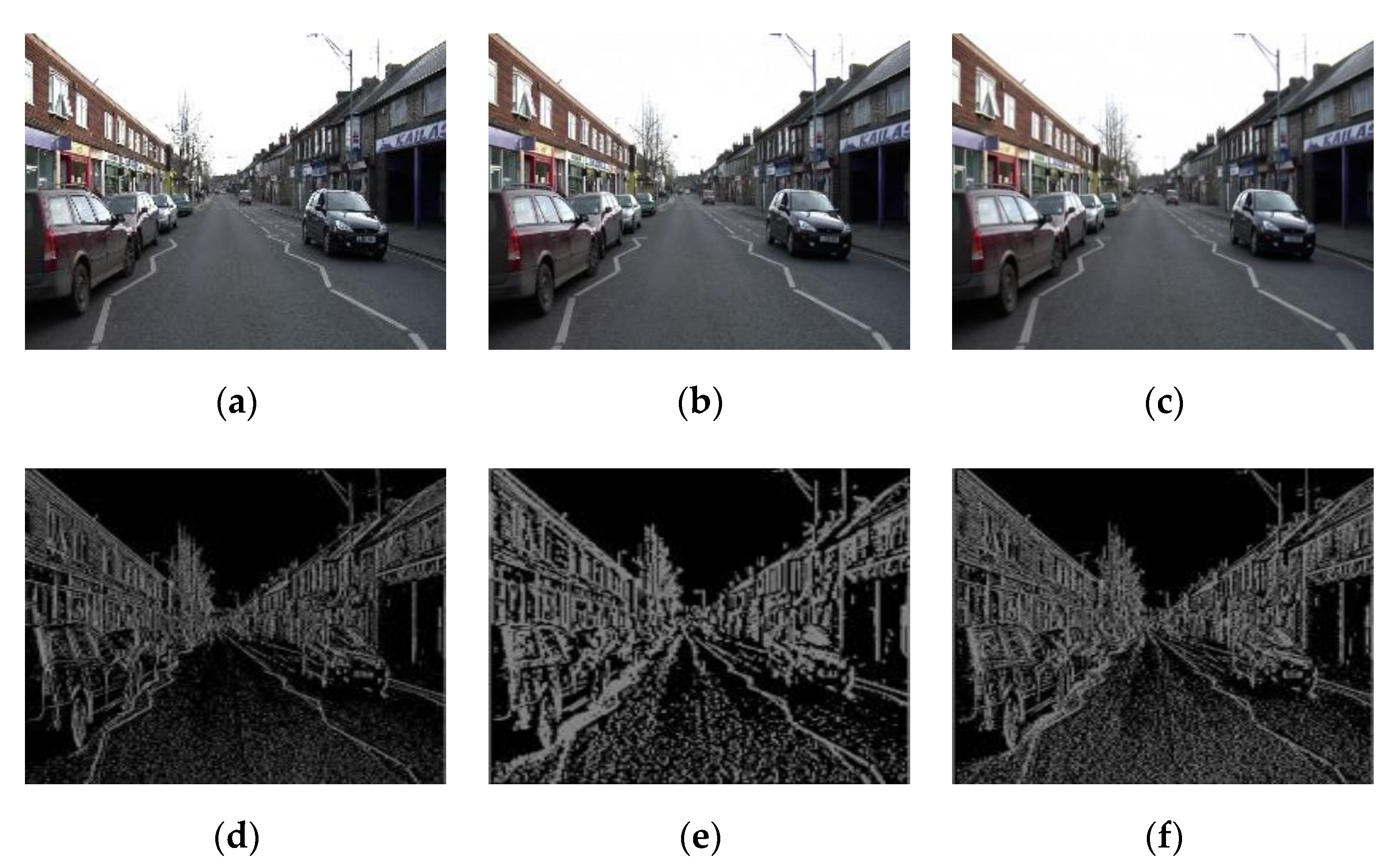
2.1. Dual Super-Resolution Learning

The Dual Super-Resolution Learning (DSRL) network is a dual super-resolution learning network based on image super-resolution in order to maintain a high-resolution display. The DSRL network aims to reconstruct high-resolution images with low-resolution input. The network model has two main modules: one is Semantic Segmentation Super-Resolution (SSSR) and the other is Single Image Super-Resolution (SISR). In addition, there is a Feature Affinity (FA) module. SSSR integrates the idea of super-resolution into the existing semantic segmentation, and the fine-grained structure based on the FA module further enhances the high-resolution features of SSSR streams. In addition, the two streams share the same feature extractor and optimize SISR branches during training.

The structure of DSRL is shown in Figure 1. The decoding module of DSRL consists of two parts. One is the SSSR module and the other is SISR, which shares the same feature extraction module. SSSR is the process of generating the final segmentation result only through upsampling; SISR is the process of image recovery from low resolution to high resolution.

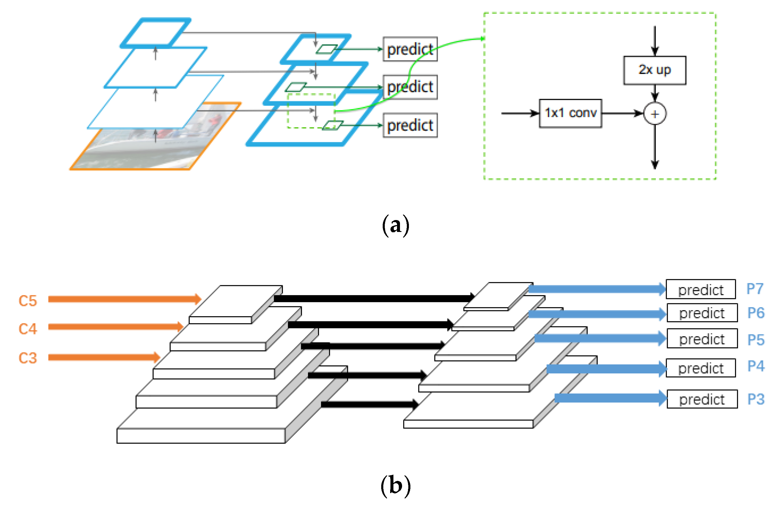
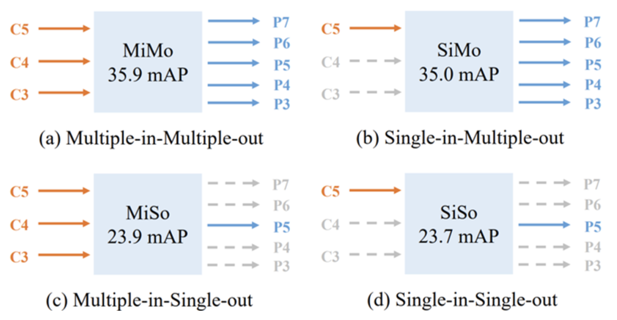
2.2. You Only Look One-Level Feature

The Feature Pyramid Network [17] (FPN) is a basic component in the recognition system used to detect objects with different scales. The FPN framework is shown in Figure 2. The main core benefits of FPN are two: on the one hand, FPN can fuse multi-scale feature maps to obtain better representation; on the other hand, it is a divide-and-conquer strategy, which detects targets on different levels of feature maps according to different scales of targets. Qian Chen [18] et al. proposed You Only Look One-level Feature. This paper studies the influence of two gain fittings of FPN on a single-stage detector. In this paper, FPN is regarded as a Multiple-in-Multiple-out (MiMo) encoder. Four types of encoders are studied: Multiple-in-Multiple-out (MiMo), Multiple-in-Single-out (MiSo), Single-in-Multiple-out (SiMo), and Single-in-Single-out (SiSo). It is found that the SiMo encoder has only one input feature, and the C5 feature layer can achieve the same performance as the MiMo encoder without feature fusion. The results are shown in Figure 3. These phenomena illustrate two facts:

(1)

C5 feature provides sufficient semantic information for object detection at different scales, which enables the SiMo encoder to achieve the same results as the MiMo encoder;

(2)

The benefit of multi-scale feature fusion is far less important than the divide-and-conquer strategy, so multi-scale feature fusion may not be the most significant benefit of FPN.

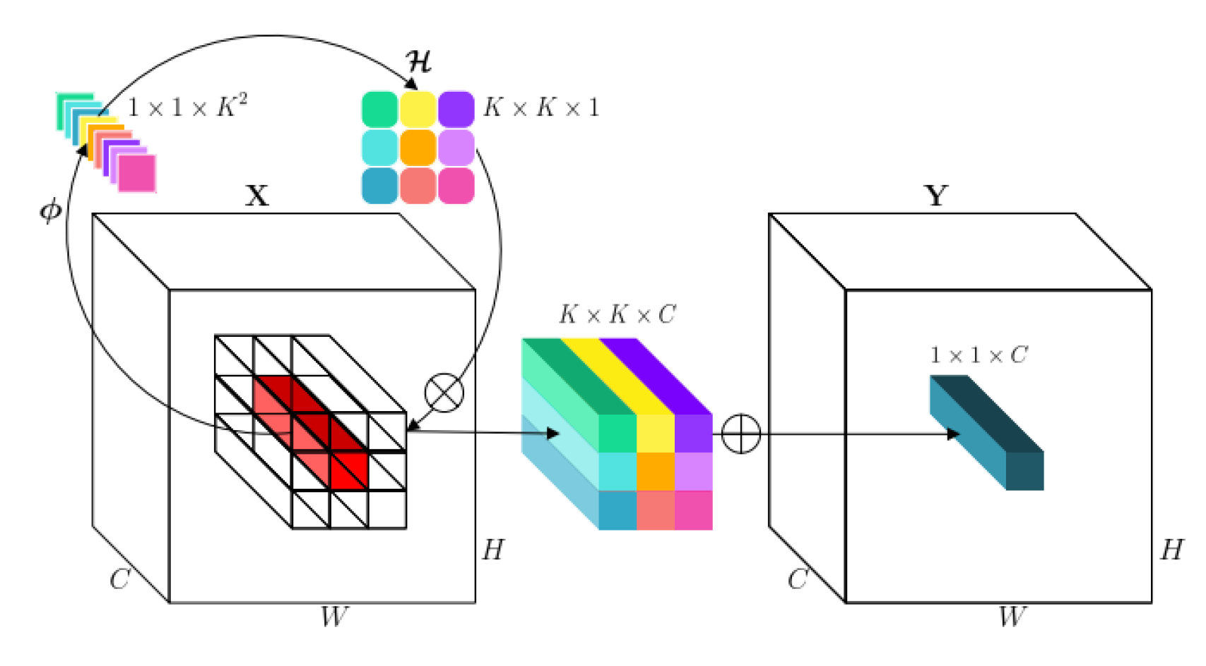
2.3. Involution

Ordinary convolution has the following two characteristics: the spatial invariance of convolution, and channel specificity. It also has two defects: one is that the receptive field is small and difficult to capture in long-distance dependence, and the other is the redundancy of information between channels. On this basis, D Li et al. proposed the concept of involution. The involution is structurally opposed to ordinary convolution. The convolution kernel is shared in the channel dimension, and the special convolution kernel in the spatial dimension can make the modeling more flexible. The structure of involution is shown in Figure 4.

The convolution kernel size of involution is $H\times W\times K\times K\times G$, among $G<<C$. This means that all channels share convolution kernels. In the involution, the fixed weight matrix is not used as in the ordinary convolution, but the corresponding involution kernel is generated according to the characteristic graph. Spatial specificity makes the convolution kernel have the ability to capture multiple feature representations at different spatial locations, and improves the problem of long-distance pixel dependence. The channel invariance performance reduces the redundant information between channels to a certain extent and improves the computing efficiency of the network. In essence, this design from ordinary convolution to internal convolution redistributes the computing power at the top level, and the essence of network design is the distribution of computing power, in order to adjust the limited computing power to the position where it can give full play to its performance. This involution module is easy to implement and can be easily combined with various network models. It can easily replace conventional convolution to realize an excellent backbone network structure.

2.4. Network Structure

In the network model of Dual Super-Resolution Learning (DSRL), in order to reduce the impact of high-resolution pictures as input on the increase of network computing, firstly, sub-sampling the high-resolution image of 960 × 720 to 480 × 360, and the picture size becomes half of the original. For the low-resolution feature layer, simple upsampling is carried out through Semantic Segmentation Super-Resolution (SSSR) and Single Image Super-Resolution (SISR) to restore to the original image size. This article compares the color pictures of the original size, 1/2 downsampling, and 1/2 downsampling + 2x upsampling; the pictures are not visually different, and we use the operator of [-1 -1 -1; -1 8 -1; -1 -1 -1] to extract the edges of the above three graphs. It can be found that the edge features extracted from the original image have more noise, but the image details are also well preserved. The edge feature noise extracted after 1/2 downsampling is reduced, but the details of the object also become rough; the edge feature noise and object details extracted after 1/2 downsampling + 2x upsampling are greatly reduced. In the following experiment, parts of these three images are used as input and the segmentation effects are compared. The experimental results show that although downsampling will reduce the noise, the missing details are more important, and the amount of noise has little effect on accuracy. Images and their respective extracted edge features as shown in Figure 5.

Therefore, this paper proposes a new network model based on the Dual Super-Resolution Learning (DSRL) network model to improve the above problems. The network is divided into two modules. One is the low-resolution image convolution module based on the super-resolution theory; the other is the convolution module of high-resolution pictures. In this paper, only the C5-level feature layer is extracted with reference to You Only Look One-level Feature (YOLOF). The C5-level feature layer has sufficient semantic information, so the low-resolution convolution module does not carry out feature fusion, expands the receptive field range through expansion convolution, and then recovers to high resolution through upsampling. However, since the image is downsampled twice at the beginning, resulting in the loss of features of the original image, a convolution module of the high-resolution image is added to the network to make up for the loss of features caused by the reduction of resolution. In order to avoid the proliferation of network parameters caused by the convolution of high-resolution images, this module only performs a small amount of convolution, and partial convolution is replaced by internal convolution to reduce the amount of calculation. The network structure is shown in Figure 6, maintaining two branches during training and two branches during testing. Pruning occurred during testing to remove Mean Square Error (MSE) loss branches and to reduce the amount of calculation.

2.5. Loss Function

The network loss function consists of three parts: one is the cross-entropy loss function composed of the network output and the actual segmentation graph, and the other is the binary-cross-entropy loss function composed of the network low-dimensional feature layer and the feature graph sampled under the actual segmentation graph to the corresponding size. The last part consists of the Mean Square Error (MSE) between the network output and the actual picture. The real segmentation’s edge features are shown in Figure 7 (edge extraction from ground truth). The Cross-Entropy (CE) loss function is shown in Formula (1). $y_i$ and $p_i$ refer to the segmentation predicted probability and the corresponding category for pixel $i$. The Binary Cross-Entropy (BCE) loss function is shown in Formula (2). $y_i$ and $x_i$ refer to the target value and the value of model output. The Mean Square Error is shown in Formula (3). $x_i$ and $y_i$ refer to the target value and the value of model output. The whole loss function is shown in Formula (4). $w_1$ and $w_2$ are set as 0.2 and 0.4.

$$L_{CE}=\frac{1}{N}{\displaystyle \sum }_{i=1}^N-y_i\log \left(p_i\right)$$

(1)

$$L_{BCE}=-\frac{1}{N}{\displaystyle \sum }_{i=1}^N\left[y_i\log x_i+\left(1-y_i\right)\log (1-x_i\right)]$$

(2)

$$L_{MSE}=\frac{1}{N}{\displaystyle \sum }_{i=1}^N\Vert x_i-y_i\Vert$$

(3)

$$L=w_1{L}_{MSE}+w_2{L}_{BCE}+L_{CE}$$

(4)

3. Results

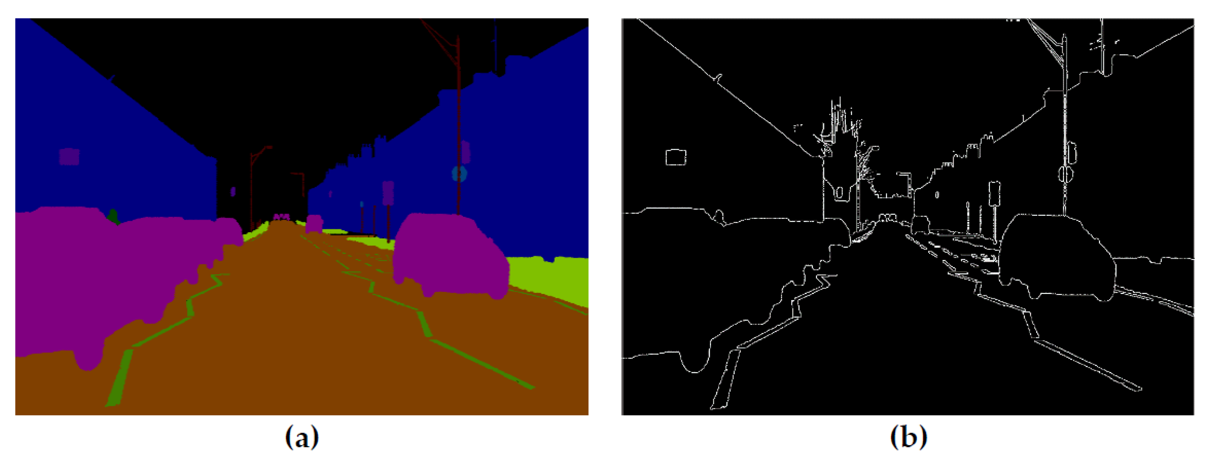
3.1. Construction of Dataset

In this paper, a CamVid (Cambridge-driving Labeled Video Database) dataset was selected, which was composed of 960 × 720 high-resolution pictures intercepted by videos taken during the real driving process of vehicles. It was divided into 32 categories, such as bicycles, roads, cars, and so on. This paper divided the training set, verification set, and test set according to the proportion of 7:2:1. In order to enhance the generalization ability of the model, data enhancement methods such as flipping and clipping were used for the training set data.

3.2. Network Model Evaluation Index

Assuming that there are $k$ classes (including $k-1$ target classes and one background class), $k-1$ represents the total number of pixels belonging to the $i$ class predicted as $j$ class, and specifically, $p_{ii}$ represents TP (true positive); $p_{ij}$ indicates FP (false positive); and $p_{ji}$ indicates FN (false negatives). The evaluation indicators included the following categories:

(1)

PA (Pixel Accuracy): The ratio between the number of pixels correctly classified and all pixel points is shown in Formula (5).

$$\mathrm{PA}=\frac{{{\displaystyle \sum }}_{i=0}^k{p}_{ii}}{{{\displaystyle \sum }}_{i=0}^k{{\displaystyle \sum }}_{j=0}^k{p}_{ij}}$$

(5)

The larger the value of the evaluation index, the more accurate the predicted pixel classification is.

(2)

MPA (Mean Pixel Accuracy) calculated the average value based on the proportion of correctly classified pixel points to all pixel points, and the formula is shown in (6).

$$\mathrm{MPA}=\frac{1}{k+1}\frac{{{\displaystyle \sum }}_{i=0}^k{p}_{ii}}{{{\displaystyle \sum }}_{i=0}^k{{\displaystyle \sum }}_{j=0}^k{p}_{ij}}$$

(6)

(3)

MIOU (Mean Intersection over Union): The ratio between the intersection between the real value and the predicted value and the union between the real value and the predicted value is averaged, and the formula is shown in (7).

$$\mathrm{MIOU}=\frac{1}{k+1}{\displaystyle \sum }_{i=0}^k\frac{p_{ii}}{{{\displaystyle \sum }}_{j=0}^k{p}_{ij}+{{\displaystyle \sum }}_{j=0}^k{p}_{ji}-p_{ii}}$$

(7)

(4)

DICE: The ratio of the intersection of 2 times the predicted result and the real result to the predicted result plus the real result is shown in Formula (8), where $X$ represents the real value, $Y$ represents the predicted value.

$$\mathrm{DICE}=\frac{2\left|X\cap Y\right|}{\left|X\right|+\left|Y\right|}$$

(8)

The larger the value of the evaluation index, the more accurate the predicted pixel classification is.

3.3. Analysis of Training Results

The framework of the neural network built in this paper was PyTorch. The model of the graphics card used was RTX2060 8G. The size of DSRL and MY network parameters in this paper are shown in

Table 1. Network model parameters.

Model	Estimated Total Size	Params Size
DSRL	8091.60 (MB)	231.03 (MB)
MY	5438.59 (MB)	40.88 (MB)

.

We compared the road classes with the largest proportion in the CamVid dataset, and the results are shown in

Table 2. Input of high-resolution network is original image.

Evaluating Indicator	DSRL	MY
IOU	91.17%	95.23%
PA	94.42%	98.99%
DICE	56.59%	60.49%

and

Table 3. Input of high-resolution network is original image and 1/2 downsampling + 2x upsampling.

Evaluating Indicator	DSRL	MY
IOU	95.23%	92.25%
PA	98.99%	97.86%
DICE	60.49%	60.25%

.

The experimental results show that the total network parameters in this paper were reduced from 8091 MB to 5438 MB. Compared with the DSRL network, the network structure in this paper improved the values of IOU, PA, and DICE:

(1)

The IOU value increased from 91.17% to 95.23%;

(2)

PA value increased from 94.42% to 98.99%;

(3)

DICE increased from 56.59% to 60.49%.

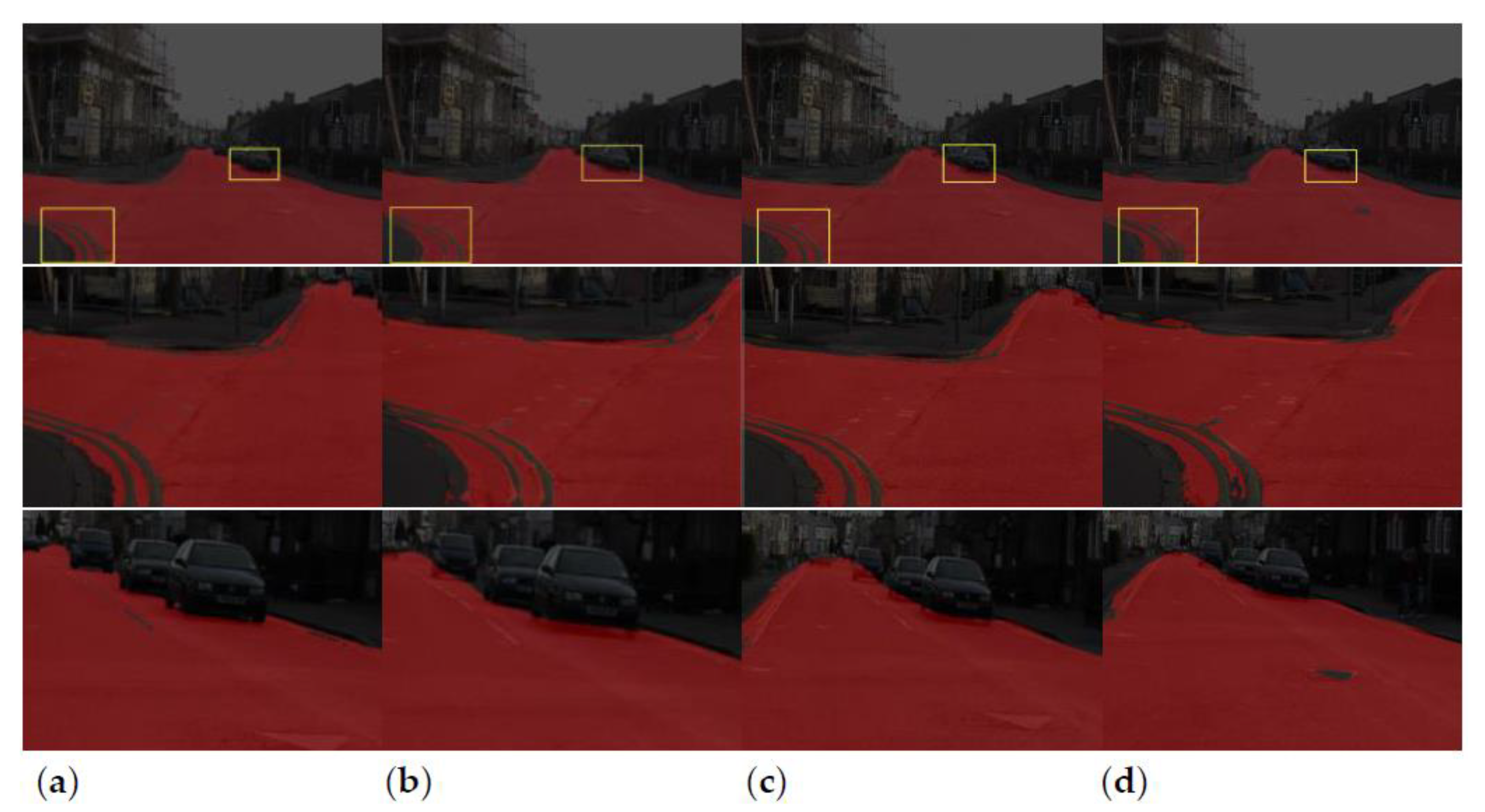
The road segmentation diagram is shown in Figure 8 (the red part is the result of road segmentation by the network, and the gray part is the standard value). The segmentation results of the DSRL network were not good for the segmentation of small objects similar to small lane lines. However, after adding the high-resolution image convolution module in this paper, the segmentation effect of small objects was improved, which shows that the high-resolution convolution module added in this model can effectively make up for the loss of the input image due to 1/2 downsampling. Although the noise will be reduced after downsampling, the priority is not as good as it is for the object details.

VGG16, ResNet101, ResNet50, and CSPdarkNet53 were used as backbone networks to compare the total network parameters, parameter size, and PA, IOU, and DICE. The results are shown in

Table 4. Network evaluation parameters and parameter sizes of various backbone networks.

Backbone	Estimated Total Size	Params Size
VGG16	3751.10 (MB)	76.87 (MB)
ResNet50	6948.62 (MB)	113.41 (MB)
ResNet101	6517.05 (MB)	185.86 (MB)
CSPDarkNet53	5438.59 (MB)	40.88 (MB)

and

Table 5. Comparison of evaluation indexes of various backbone networks.

Backbone	IOU	PA	DICE
VGG16	94.38%	96.51%	60.21%
ResNet50	92.25%	97.65%	60.25%
ResNet101	91.44%	96.55%	60.22%
CSPDarkNet53	95.23%	96.55%	60.49%

.

It can be seen from Table 4 and Table 5 that the network model with VGG16 as the backbone network could reach IOU, PA, and DICE similarly to the network model with ResNet50 and ResNet101 as the backbone network with less parameters. Taking the original image as the high-resolution network input, the comparison of various backbone network segmentation images is shown in Figure 9 (the red part is the result of the segmentation of the road class by the network).

As can be seen from various backbone network segmentation pictures in Figure 9 (the red part is the result of the segmentation of the road class by the network):

(1)

The network with VGG16 as the backbone can be achieved with half as few parameters than ResNet50 and ResNet101 with a similar effect. In terms of the segmentation accuracy of the lane line part of the road, the accuracy of VGG16 and ResNet50 is similar. Both lane lines can be clearly segmented, which is better than ResNet101. In terms of the segmentation accuracy of the tire shape at the bottom of the car, the segmentation accuracy of VGG16 is slightly better than ResNet50 and ResNet101, which can better fit the tire shape.

(2)

The tire shape segmentation accuracy of the network with CSPdarkNet53 as the backbone is better than VGG16, ResNet50, and ResNet101 on the lane line and the bottom of the vehicle, and fits better with the lane line and tire shape.

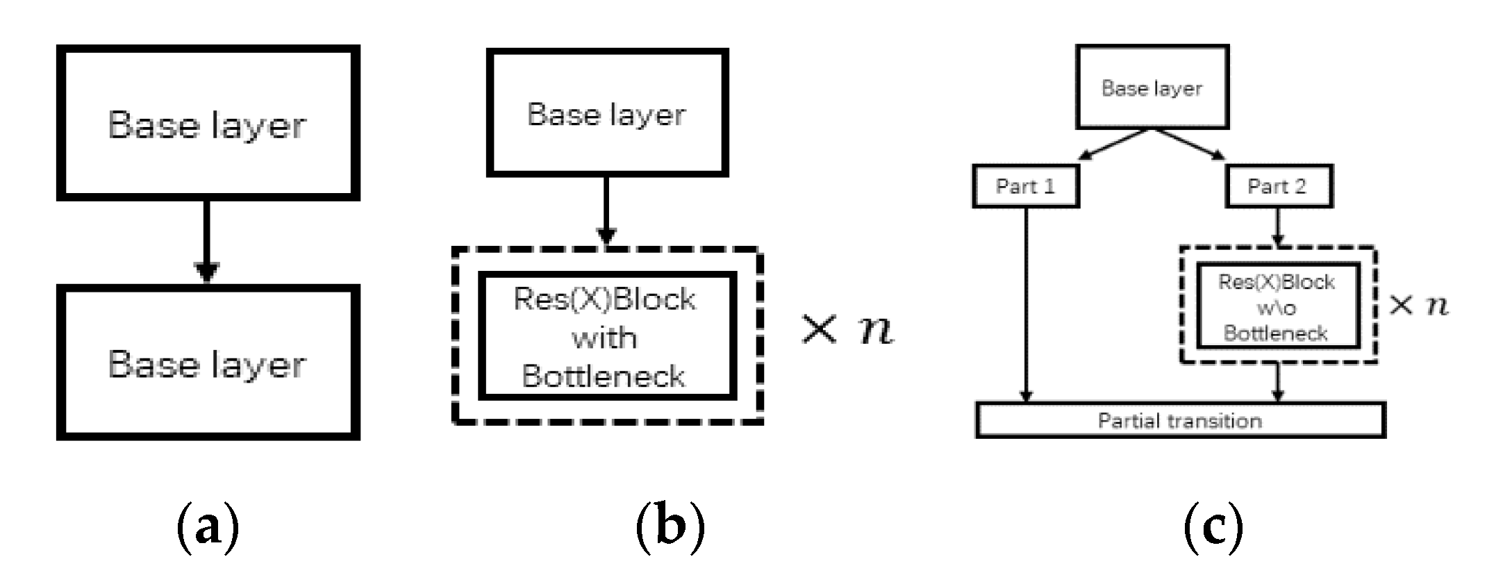
Comparing ordinary convolution, ResNet, and CSPdarknet (the above three convolution structures are shown in Figure 10), it can be found that CSPdarknet cuts the input feature map to the channel, and only uses half of the original feature map to input into the residual network for processing. In forward propagation, the other half is directly spliced by the channel with the output of the residual network at the end. The advantages of doing this are as follows:

(1)

Only half of the input is involved in the calculation, which can greatly reduce the amount of calculation and memory consumption;

(2)

In the process of back propagation, a completely independent gradient propagation path is added, which can prevent feature loss caused by excessive convolution, and there is no reuse of gradient information.

Take a video shot while driving using a single RTX2060 8G graphics card as an example: the video FPS is 25 frames, and the video resolution is 1920 × 1080, for a total of 12 s. The DSRL network takes 120 s; our network takes 65 s, a 46% reduction in time. The comparison of the segmentation results between the DSRL network and our network (the red part is the actual segmentation result) is shown in Figure 11:

It can be seen from the above two sets of comparison charts that the fps of the DSRL network can only reach about 2 frames (up to 2.31 frames) in the actual driving video, whereas our network can achieve about 4 frames (up to 4.5 frames). The segmentation is smoother. From the above pictures, we can see that our network segmentation is faster and more accurate, and the segmentation effect is better for detailed parts such as lane lines.

Taking a single image with a resolution of 960 × 720 as input, a speed comparison between DSRL and our network segmentation is shown in

Table 6. The speed comparison between DSRL and our network segmentation.

Network	DSRL	MY
Picture1	1.36(s)	1.11(s)
Picture2	2.05(s)	1.70(s)
Picture3	2.25(s)	1.71(s)
Picture4	2.50(s)	1.72(s)
Picture5	2.16(s)	1.73(s)

. From the comparison in Table 6, we can see that the time used by our network is reduced compared with the DSRL network.

4. Conclusions

In view of the high demand for hardware equipment for training and using high-resolution atlases, this paper proposes a new network model based on Dual Super-Resolution Learning (DSRL), an added high-resolution convolution module, and a discarded Feature Pyramid Network (FPN), which can effectively compensate for the downsampling of high-resolution images while reducing the amount of computation. Features are missing, and the study found that downsampling reduces noise as a lower priority than details in the picture. Our network model can segment small features better than the DSRL network, and has lower hardware requirements and faster processing speed. In terms of the actual driving video segmentation time, time is reduced by 46%, from 120 s to 65 s, which can be used in actual driving. The recognition is smoother and more accurate during driving, which greatly reduces the delay caused by high-resolution input during actual driving, thus proving the effectiveness of our method. However, the delay still exists, the detailed segmentation of objects is still lacking, and the network structure can continue being improved.

References

1. Saleh, M.; Hatzopoulou, M. Greenhouse gas emissions attributed to empty kilometers in automated vehicles. Transp. Res. Part D Transp. Environ. 2020, 88, 102567. [Google Scholar] [CrossRef]
2. Gawron, J.H.; Keoleian, G.A.; De Kleine, R.D.; Wallington, T.J.; Kim, H.C. Deep decarbonization from electrified autonomous taxi fleets: Life cycle assessment and case study in Austin, TX. Transp. Res. Part D Transp. Environ. 2019, 73, 130–141. [Google Scholar] [CrossRef]
3. Ronneberger, O.; Fischer, P.; Brox, T. U-net: Convolutional networks for biomedical image segmentation. In Proceedings of the International Conference on Medical Image Computing and Computer-Assisted Intervention, Munich, Germany, 5–9 October 2015; Springer: Cham, Switzerland, 2015; pp. 234–241. [Google Scholar]
4. Chen, L.C.; Papandreou, G.; Kokkinos, I.; Murphy, K.; Yuille, A.L. Semantic image segmentation with deep convolutional nets and fully connected crfs. arXiv 2014, arXiv:1412.7062. [Google Scholar]
5. Chen, L.C.; Papandreou, G.; Kokkinos, I.; Murphy, K.; Yuille, A.L. Deeplab: Semantic image segmentation with deep convolutional nets, atrous convolution, and fully connected crfs. IEEE Trans. Pattern Anal. Mach. Intell. 2017, 40, 834–848. [Google Scholar] [CrossRef] [PubMed] [Green Version]
6. Chen, L.C.; Zhu, Y.; Papandreou, G.; Adam, H.; Schroff, F. Encoder-decoder with atrous separable convolution for semantic image segmentation. In Proceedings of the European Conference on Computer Vision (ECCV), Munich, Germany, 8–14 September 2018; pp. 801–818. [Google Scholar]
7. Zhao, H.; Shi, J.; Qi, X.; Wang, X.; Jia, J. Pyramid scene parsing network. In Proceedings of the IEEE Conference on Computer Vision and Pattern Recognition, Honolulu, HI, USA, 21–26 June 2017; pp. 2881–2890. [Google Scholar]
8. Badrinarayanan, V.; Kendall, A.; Cipolla, R. Segnet: A deep convolutional encoder-decoder architecture for image segmentation. IEEE Trans. Pattern Anal. Mach. Intell. 2017, 39, 2481–2495. [Google Scholar] [CrossRef] [PubMed]
9. Yu, J.; Yu, Z. Mono-Vision Based Lateral Localization System of Low-Cost Autonomous Vehicles Using Deep Learning Curb Detection. Actuators 2021, 10, 57. [Google Scholar] [CrossRef]
10. Mehta, S.; Rastegari, M.; Caspi, A.; Shapiro, L.; Hajishirzi, H. Espnet: Efficient spatial pyramid of dilated convolutions for semantic segmentation. In Proceedings of the European Conference on Computer Vision (ECCV), Munich, Germany, 8–14 September 2018; pp. 552–568. [Google Scholar]
11. Mehta, S.; Rastegari, M.; Shapiro, L.; Hajishirzi, H. Espnetv2: A light-weight, power efficient, and general purpose convolutional neural network. In Proceedings of the IEEE/CVF Conference on Computer Vision and Pattern Recognition, Long Beach, CA, USA, 15–20 June 2019; pp. 9190–9200. [Google Scholar]
12. Sandler, M.; Howard, A.; Zhu, M.; Zhmoginov, A.; Chen, L.C. Mobilenetv2: Inverted residuals and linear bottlenecks. In Proceedings of the IEEE Conference on Computer Vision and Pattern Recognition, Salt Lake City, UT, USA, 18–23 June 2018; pp. 4510–4520. [Google Scholar]
13. Ma, N.; Zhang, X.; Zheng, H.T.; Sun, J. Shufflenet v2: Practical guidelines for efficient cnn architecture design. In Proceedings of the European Conference on Computer Vision (ECCV), Munich, Germany, 8–14 September 2018; pp. 116–131. [Google Scholar]
14. Han, S.; Mao, H.; Dally, W.J. Deep compression: Compressing deep neural networks with pruning, trained quantization and huffman coding. arXiv 2015, arXiv:1510.00149. [Google Scholar]
15. Li, D.; Hu, J.; Wang, C.; Zhu, L.; Zhang, T.; Chen, Q. Involution: Inverting the inherence of convolution for visual recognition. In Proceedings of the IEEE/CVF Conference on Computer Vision and Pattern Recognition, Nashville, TN, USA, 20–25 June 2021; pp. 12321–12330. [Google Scholar]
16. Wang, L.; Li, D.; Zhu, Y.; Shan, Y.; Tian, L. Dual super-resolution learning for semantic segmentation. In Proceedings of the IEEE/CVF Conference on Computer Vision and Pattern Recognition, Seattle, WA, USA, 13–19 June 2020; pp. 3774–3783. [Google Scholar]
17. Kim, S.W.; Kook, H.K.; Sun, J.Y.; Kang, M.C.; Ko, S.J. Parallel feature pyramid network for object detection. In Proceedings of the European Conference on Computer Vision (ECCV), Munich, Germany, 8–14 September 2018; pp. 234–250. [Google Scholar]
18. Chen, Q.; Wang, Y.; Yang, T.; Zhang, X.; Cheng, J.; Sun, J. You only look one-level feature. In Proceedings of the IEEE/CVF Conference on Computer Vision and Pattern Recognition, Nashville, TN, USA, 20–25 June 2021; pp. 13039–13048. [Google Scholar]
Figure 1. Dual Super-Resolution Learning (DSRL) network structure: (a) DSRL network structure; (b) Semantic Segmentation Super-Resolution (SSSR) realizes image segmentation only by upsampling; (c) SSSR + Single Image Super-Resolution (SISR) restore from low-resolution feature layer to high resolution of original image.
Actuators 11 00069 g001
Figure 2. Feature Pyramid Networks (FPN) network structure: (a) FPN overall network structure; (b) The last three layers of the feature extraction module are C3~C5, respectively, and the prediction modules are P3~P7, respectively.
Actuators 11 00069 g002
Figure 3. Results of four input and output combinations of FPN. Using C3~C5 level feature layers of the backbone and the feature layers of P3~P7 as the final output, compare the mAP (mean Average Precision) indicators of the four decoders: (a) MiMo; (b) SiMo; (c) MiSo; (d) SiSo.
Actuators 11 00069 g003
Figure 4. Involution structure (the involution kernel H i , j K × K × 1 ( G = 1 in this example for ease of demonstration) is yielded from the function ϕ conditioned on a single pixel at i , j , followed by a channel-to-space rearrangement. The multiply–add operation of involution is decomposed into two steps, with indicating multiplication broadcast across C channels and indicating summation aggregated within the K × K spatial neighborhood).
Actuators 11 00069 g004
Figure 5. Picture features: (a) Original RGB picture; (b) 1/2 downsampling RGB picture; (c) 1/2 downsampling + 2x upsampling RGB picture; (d) Original RGB picture’s edge features; (e) 1/2 downsampling RGB picture′s edge features; (f) 1/2 downsampling + 2x upsampling RGB picture′s edge features.
Actuators 11 00069 g005
Figure 6. Network structure: (a) MY network structure; (b) Low-resolution convolution module; (c) High-resolution module convolution module.
Actuators 11 00069 g006
Figure 7. (a) Ground truth segmentation; (b) Edge features of real segmentation.
Actuators 11 00069 g007
Figure 8. Road segmentation picture: (a) DSRL (b) MY (1/2 downsampling + 2x upsampling) (c) MY (original picture) (d) Ground Truth.
Actuators 11 00069 g008
Figure 9. Comparison of various backbone network segmentation pictures: (a) CSPDarknet53; (b) VGG16; (c) ResNet50; (d) ResNet101.
Actuators 11 00069 g009
Figure 10. Convolutional structure: (a) Ordinary convolution; (b) ResNet; (c) CSPdarknet.
Actuators 11 00069 g010
Figure 11. Comparison of the segmentation results of the DSRL network and our own network (the red part is the actual segmentation result). (a,c,e) are the segmentation results of our network on the video; (b,d,f) are the segmentation results of DSRL network at the same time point of the same video.
Actuators 11 00069 g011