Optimal Control Method of Path Tracking for Four-Wheel Steering Vehicles

Abstract

Path tracking is a key technique for intelligent electric vehicles, while four-wheel steering (4WS) technology is of great significance to improve its accuracy and flexibility. However, the control methods commonly used in path tracking for a 4WS vehicle cannot take full advantage of the additional steering freedom of the 4WS vehicle, because of restricting the relationship between the front and rear wheels steering angle. To address this issue, we derive a kinematic model without the restriction based on the small-angle assumption. Then, the objective function and constraints of system control quantity optimization are designed based on the tracking error model. After the optimization problem is solved in the form of quadratic programming with constraints, the control sequence with the smallest performance index is obtained through rolling optimization. The proposed method is tested on a high-fidelity Carsim/Simulink co-simulation platform and an experimental vehicle. The results show that the standard deviation of the lateral error and the yaw angle error of the algorithm is less than 0.1 m and 3.0°, respectively. Compared with the other two algorithms, the control of the front and rear wheels angle of this method is more flexible and the tracking accuracy is higher.

1. Introduction

In recent years, unmanned vehicles have become a research hotspot due to the increase of various traffic problems such as traffic congestion and traffic accidents [1]. The key technologies mainly include environmental perception, precise localization, planning and decision-making, and motion control. Path tracking is one of the key problems of motion control for autonomous vehicles, which is denoted as tracking a predetermined path by controlling the lateral and yaw movement of the vehicle [2]. Thus, it can be defined as minimizing the lateral offset and heading errors [3].

Path tracking control methods can be mainly divided into two categories. One is geometry-based, which mainly includes pure pursuit (PP) [4] and Stanley [5], etc. The other is model-based, represented by synovial membrane control [6], linear quadratic regulator (LQR) [7,8] and model predictive control (MPC) [9,10], etc. Geometry-based control methods are often used in low-speed scenarios, with good interpretability and fast calculation speed. Model-based methods mainly based on dynamic models are often used for stability control of high-speed vehicles [11], whose disadvantages include poor real-time performance and the difficulty to obtain kinetic parameters accurately [12]. However, the above studies are mostly based on front-wheel steering (FWS) vehicles. The only control input for lateral tracking control is the front-wheel steering angle, which limits the ability of path tracking control.

To improve the flexibility and stability of vehicles, the concept of the 4WS vehicle was proposed in the late 1980s [13]. At low speed, the steering modes of a 4WS vehicle are more diverse than FWS vehicles [14,15]. The front and rear wheels can be turned in reverse phase to reduce the turning radius and improve maneuverability. At high speed, a 4WS vehicle can improve handling stability by steering the front and rear wheels in phase to ensure zero slip angle and ideal yaw rate [16]. Making full use of the additional degrees of freedom of the 4WS vehicle can independently control the path and attitude of the vehicle, reduce the yaw motion required by the body, and improve the responsiveness of the vehicle heading change [2]. At the same time, the vehicle has better path tracking performance due to the improvement of flexibility [17].

Aiming at the path tracking problem of the 4WS vehicle, Ye et al. [18] designed a strategy to switch steering modes include active front and rear steering (AFRS), Ackermann steering, and crab steering for achieving accurate path-following of the vehicle. Hiraoka et al. [6] proposed a 4WS vehicle path tracking controller based on the sliding mode control theory, which uses front and rear control points for tracking. However, the above methods restrict the steering freedom of the 4WS vehicle and reduce flexibility. Wu et al. [19] developed a novel rear-steering-based decentralized control (RDC) algorithm for the 4WS vehicle. Yin et al. [20] carried out a new distribution controller to allocate driving torques to four-wheel motors, which can use each tire to generate yaw moment and achieve a quicker yaw response. Fnadi et al. [21] synthesized a new controller for dynamic path tracking by using constrained model predictive control (MPC) for double steering off-road vehicles, which takes into account steering and sliding constraints to ensure safety and lateral stability. However, these methods only use rear-wheel steering within a small turning angle range and are not suitable for flexible control of 4WS vehicle at low speed.

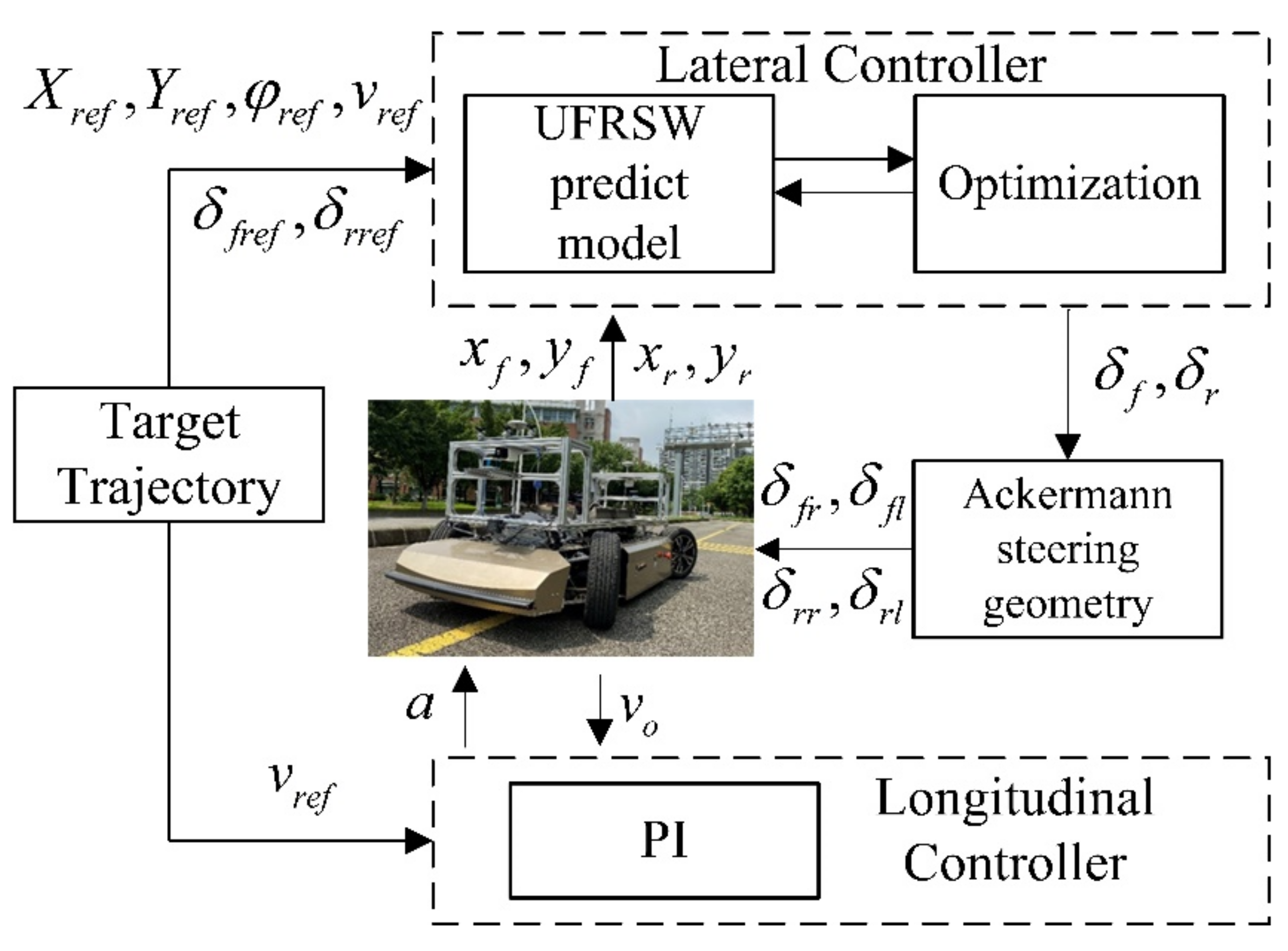
Aiming at these challenges, a tracking error model unrestrained on the front and rear wheels steering (UFRWS) relationship of the 4WS vehicle is established in this paper. As shown in Figure 1, a predictive controller based on this model is proposed, which performs lateral motion control, and forms a trajectory tracking controller with the PI controller that performs longitudinal control. The advantage of this controller is that it can fully utilize the steering freedom of the 4WS vehicle, improving tracking accuracy and flexibility.

2. Kinematics Model of 4WS Vehicle

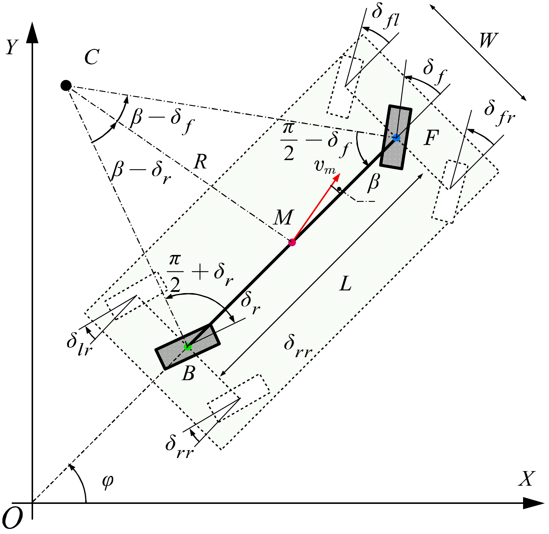
The kinematic model is the basis of trajectory planning and tracking control. To reduce the complexity of the controller design, the 4WS vehicle kinematics model can be simplified to a single-track model with the assumption of pure rolling and small steering angle as shown in Figure 2. The points $F(x_f,y_f)$ and $B(x_{\mathrm{r}},y_r)$ are the center of the front and the rear axle of the vehicle, respectively. The point $M(x,y)$ is the geometric center of the vehicle, and the point $C$ is the center of rotation of the vehicle.$R$ denotes the radius of rotation of the vehicle. The wheelbase L is the distance between the front and rear axles, and the wheel track $W$ refers to the distance between the left and right wheels. The heading angle $\phi$ refers to the angle between the body direction and the $X$ axis in the global coordinate system $XOY$. The center of mass slip angle $\beta$ is the angle between the speed $v_m$ at the point $M$ and the direction of the body.

The 4WS vehicle bicycle model is gray as shown in Figure 2. Its front steering angle ${\delta }_f$ and rear steering angle ${\delta }_r$ should satisfy the Ackerman steering geometric relationship. So, the steering angle of each wheel ${\delta }_i(i=fr,fl,rr,rl)$ satisfies the Equation (1).

$$\begin{array}{l}\left\{\begin{array}{l}\tan {\delta }_{fl}=\frac{\tan {\delta }_f}{1-\frac{W}{2L}(\tan {\delta }_f-\tan {\delta }_r)}\\ \tan {\delta }_{fr}=\frac{\tan {\delta }_f}{1+\frac{W}{2L}(\tan {\delta }_f-\tan {\delta }_r)}\\ \tan {\delta }_{rl}=\frac{\tan {\delta }_r}{1-\frac{W}{2L}(\tan {\delta }_f-\tan {\delta }_r)}\\ \tan {\delta }_{rr}=\frac{\tan {\delta }_r}{1+\frac{W}{2L}(\tan {\delta }_f-\tan {\delta }_r)}\end{array}\right.\\ \end{array}$$

(1)

We take M as the control point. Then, the nonlinear kinematics equations of the 4WS vehicle bicycle model in the global coordinate system can be expressed as

$$\left\{\begin{array}{l}\dot{X}=v_m\cos (\phi +\beta )\\ \dot{Y}=v_m\sin (\phi +\beta )\\ \dot{\phi }=\frac{v_m\cos (\beta )}{L}\left(\tan \left({\delta }_f\right)-\tan \left({\delta }_r\right)\right)\\ \beta =\arctan \left(\frac{\tan {\delta }_r+\tan {\delta }_f}{2}\right)\end{array}\right.$$

(2)

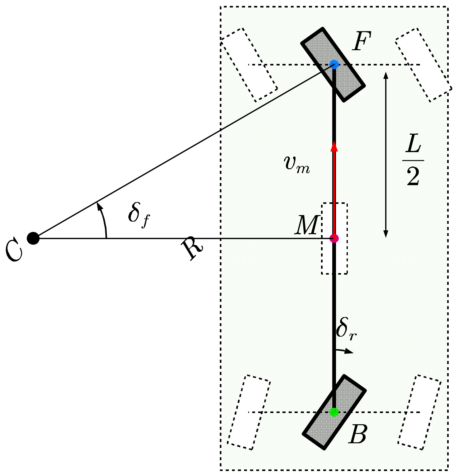
Most of the existing path tracking lateral control methods are designed for the application of front-wheel steering vehicles. Therefore, to apply PP and MPC methods to four-wheel steered vehicles, this article regards 4WS as FWS vehicles with the wheelbase halved by restricting the steering angles of the front and the rear to be equal and out of phase as shown in Figure 3. Then, Equation (2) can be simplified to Equation (3), which is the symmetrical front and the rear wheels steering (SFRWS) model of the 4WS vehicle. The PP and MPC methods based on the SFRWS model can be used as the comparison algorithm in this article for the method based UFRWS model.

$$\left\{\begin{array}{l}\dot{X}=v_m\cos \phi \\ \dot{Y}=v_m\sin \phi \\ \dot{\phi }=2v_m\tan {\delta }_f/L\end{array}\right.$$

(3)

Obviously, due to the constraint between the front and rear wheel angle relationship, the SFRWS model limits the steering freedom of 4WS vehicle, which reduces flexibility. For this reason, this paper proposes a predictive control method based on the unconstrained steering model of 4WS.

From the trigonometric function operation, we can get the Equation (4).

$$\tan {\delta }_r+\tan {\delta }_f=\tan ({\delta }_f+{\delta }_r)(1-\tan {\delta }_r\tan {\delta }_f)$$

(4)

We can further simplify the kinematics model because the vehicle turning angle is less than 30°.

$$\tan {\delta }_r+\tan {\delta }_f\approx ({\delta }_f+{\delta }_r)$$

(5)

Combining Equations (1) and (5), we can get a simplified non-linear 4WS kinematics model unrestrained on the front and the rear wheel steering relationship (UFRWS). The model is as follows:

$$\begin{array}{l}\dot{X}=V\cos (\psi +\left(\frac{{\delta }_r+{\delta }_f}{2}\right))\\ \dot{Y}=V\sin (\psi +\left(\frac{{\delta }_r+{\delta }_f}{2}\right))\\ \dot{\psi }=\frac{V\cos \left(\frac{{\delta }_r+{\delta }_f}{2}\right)}{{\ell }_f+{\ell }_r}\left({\delta }_f-{\delta }_r\right)\end{array}$$

(6)

3. Optimal Predictive Control Based Different Model

In this section, the objective functions and constraints of system control quantity optimization are designed based on the UFRWS model and SFRWS model. The optimization problem is solved in the form of a constrained quadratic programming and rolling optimization is performed.

3.1. Linear Discrete Tracking Error Model Based UFRWS Model

We define the state vector $\chi ={[\begin{array}{ccc}{e}_x& e_y& e_{\phi }\end{array}]}^T$, the control input $u={[\begin{array}{cc}{\delta }_f& {\delta }_r\end{array}]}^T$, where the error $e_x$ is the difference between the actual position of the vehicle and the reference position in the $X$ direction, the error $e_y$ is in the Y direction, and the heading error $e_{\phi }$ is the difference between the vehicle heading angle and the reference heading angle. Then, the tracking error model based on UFRWS model can be obtained.

$$\dot{\chi }=\left[\begin{array}{l}{\dot{e}}_x\\ {\dot{e}}_y\\ {\dot{e}}_{\phi }\end{array}\right]=\left[\begin{array}{l}\dot{X}-{\dot{X}}_{ref}\\ \dot{Y}-{\dot{Y}}_{ref}\\ \dot{\phi }-{\dot{\phi }}_{ref}\end{array}\right]=f(\chi ,u)$$

(7)

Since the reference points are all on the reference trajectory, Equation (7) can be expanded by the first-order Taylor expansion at the reference state quantity ${\chi }_{ref}={[\begin{array}{ccc}0& 0& 0\end{array}]}^T$, and we can get:

$$\dot{\chi }={\left.\frac{\partial f(\chi ,u)}{\partial \chi }\right|}_{\begin{array}{c}\chi ={\chi }_{ref},\\ u=u_{ref}\end{array}}\left(\chi -{\chi }_{ref}\right)+{\left.\frac{\partial f(\chi ,u)}{\partial u}\right|}_{\begin{array}{c}\chi ={\chi }_{ref},\\ u=u_{ref}\end{array}}\left(u-u_{ref}\right)$$

(8)

Based on the Jacobi matrix, the state space form of the linear tracking error model can be developed as follows:

$$\left\{\begin{array}{l}\dot{\chi }=A\chi +Bu+W\\ \eta =C\chi \end{array}\right.,$$

(9)

where $\eta$ is the state transition matrix, $C$ is the $3\times 3$ identity matrix.

Discretizing the continuous system Equation (9) by using the forward Euler method can obtain a linear discrete tracking error model Equation (10).

$$\chi (k+1)=A_d\chi (k)+B_{d}u(k)+W_d,$$

(10)

Where $A_d=I+AT=\left[\begin{array}{ccc}1& 0& -T{v}_{ref}\sin \left({\phi }_{ref}+{\beta }_{ref}\right)\\ 0& 1& T{v}_{ref}\cos \left({\phi }_{ref}+{\beta }_{ref}\right)\\ 0& 0& 1\end{array}\right]$, $B_d=BT=\left[\begin{array}{cc}-\frac{1}{2}T{v}_{ref}\sin \left({\phi }_{ref}+{\beta }_{ref}\right)& -\frac{1}{2}T{v}_{ref}\sin \left({\phi }_{ref}+{\beta }_{ref}\right)\\ \frac{1}{2}T{v}_{ref}\cos \left({\phi }_{ref}+{\beta }_{ref}\right)& \frac{1}{2}T{v}_{ref}\cos \left({\phi }_{ref}+{\beta }_{ref}\right)\\ -T{v}_{ref}\frac{sin{\beta }_{ref}\left({\delta }_f-{\delta }_r\right)-cos{\beta }_{ref}}{2L}& -T{v}_{ref}\frac{sin{\beta }_{ref}\left({\delta }_f-{\delta }_r\right)+cos{\beta }_{ref}}{2L}\end{array}\right]$, $W_d=WT=\left[\begin{array}{c}\frac{1}{2}{v}_{ref}\sin \left({\phi }_{ref}+{\beta }_{ref}\right)({\delta }_f+{\delta }_r)T\\ -\frac{1}{2}{v}_{ref}\cos \left({\phi }_{ref}+{\beta }_{ref}\right)({\delta }_f+{\delta }_r)T\\ \frac{1}{2}{\delta }_f{v}_{ref}(\sin {\beta }_{ref}({\delta }_f-{\delta }_r)-cos{\beta }_{ref})T/L+\frac{1}{2}{\delta }_r{v}_{ref}(\sin {\beta }_{ref}({\delta }_f-{\delta }_r)+cos{\beta }_{ref})T/L\end{array}\right]$.

3.2. Linear Discrete Tracking Error Model Based SFRWS Model

Different from the UFRWS-based model, the control input of the SFRWS-based system is only the front wheel angle, that is $u={\delta }_f$. In the same way, the discretization model based SFRWS model can be obtained as follows:

$$\chi (k+1)=A_d\chi (k)+B_{d}u(k)+W_d,$$

(11)

where $A_d=\left[\begin{array}{ccc}1& 0& -T{v}_{ref}\sin \left({\phi }_{ref}\right)\\ 0& 1& T{v}_{ref}\cos \left({\phi }_{ref}\right)\\ 0& 0& 1\end{array}\right]$,$B_d=\left[\begin{array}{c}0\\ 0\\ \frac{T{v}_{ref}}{L{\cos }^2{\delta }_f}\end{array}\right]$,$W_d=WT=\left[\begin{array}{c}0\\ 0\\ -\frac{T{v}_{ref}{\delta }_f}{L{\cos }^2{\delta }_f}\end{array}\right]$.

3.3. State Prediction Model

According to Equation (11), the state quantity at each moment can be predicted.

$$\begin{array}{l}\chi (k+1\left|k\right.)=A_d\chi (k)+B_{d}u(k)+W_d\\ \chi (k+2\left|k\right.)=A_d{}^2\chi (k)+A_d{B}_{d}u(k)+B_{d}u(k+1)+A_d{W}_d+W_d\\ \chi (k+3\left|k\right.)=A_d{}^3\chi (k)+A_d^2{B}_{d}u(k)+A_d{B}_{d}u(k+1)+B_{d}u(k+2)+A_d^2{W}_d+A_d{W}_d+W_d\\ \begin{array}{cc}& \end{array}⋮\\ \chi (k+N_p\left|k\right.)=A_d{}^{N_p}\chi (k)+A_d^{N_p-1}{B}_{d}u(k)+\dots +A_d^{N_p-N_c-1}{B}_{d}u(k+N_c)+A_d^{N_P-1}{W}_d+\dots +A_d^{N_p-N_p}{W}_d\end{array}$$

(12)

Then, the state prediction equation is:

$$Y(k)=\Psi \chi (k)+\Theta U(k)+W_e,$$

(13)

where $Y(k)=\left[\begin{array}{c}\eta (k+1\left|k\right.)\\ \eta (k+2\left|k\right.)\\ \eta (k+3\left|k\right.)\\ \cdots \\ \eta (k+N_p\left|k\right.)\end{array}\right]$, $U(k)=\left[\begin{array}{c}u(k\left|k\right.)\\ u(k+1\left|k\right.)\\ u(k+2\left|k\right.)\\ \cdots \\ u(k+N_c\left|k\right.)\end{array}\right]$, $\Psi =\left[\begin{array}{c}C{A}_d\\ C{A}_d{}^2\\ C{A}_d{}^3\\ \cdots \\ C{A}_d{}^{N_p}\end{array}\right]$,

$\Theta =\left[\begin{array}{cccc}C{B}_d& & & \\ C{A}_d{B}_d& C{B}_d& & \\ C{A}_d{}^2{B}_d& C{A}_d{B}_d& C{B}_d& \\ \cdots & & & \\ C{A}_d{}^{N_p-1}{B}_d& C{A}_d{}^{N_p-2}{B}_d& \cdots & C{A}_d{}^{N_p-N_c-1}{B}_d\end{array}\right]$$W_e=\left[\begin{array}{c}C{W}_d\\ C{A}_d{W}_d+C{W}_d\\ C{A}_d^2{W}_d+C{A}_d{W}_d+C{W}_d\\ ⋮\\ C{A}_d^{k-1}{W}_d+C{A}_d^{k-2}{W}_d+\cdots +C{W}_d\end{array}\right]$.

3.4. Scrolling Optimization

The control goal of the system is to make the 4WS vehicle track the target trajectory quickly and stably. Therefore, it is necessary to optimize the state quantity of the system, the control quantity, and the amount of change in the control quantity.

At the $k$ moment, the amount of change in the control quantity is defined as:

$$\Delta u(k)=u(k)-u(k-1).$$

(14)

Then:

$$\Delta U(k)=\left[\begin{array}{c}\Delta u(k)\\ \Delta u(k+1)\\ \cdots \\ \Delta u(k+N_c)\end{array}\right]=\left[\begin{array}{cccc}1& -1& & \\ -1& 1& & \\ & & \dots & \\ & & -1& 1\end{array}\right]U=DU.$$

(15)

The design objective function is as follows:

$$J(k)={\displaystyle \sum _{i=1}^{N_p}{‖\chi (k+i)‖}_Q^2}+{\displaystyle \sum _{i=1}^{N_c-1}{‖U(k+i)-U_{ref}(k+i)‖}_{R_1}^2}+{\displaystyle \sum _{i=1}^{N_c-1}{‖\Delta U(k+i)‖}_{\Delta R}^2},$$

(16)

where the first part is to make the current state error that is the lateral error and heading error close to 0. The importance of each state quantity can be adjusted by changing the weight value in the matrix $R$. The second part is to minimize the error between the control quantity and the reference value. The weight of each control variable can be set by adjusting the weight value in the matrix $R_1$. The third part is to make the change of the control variable as small as possible to reduce the output angular velocity value. The parameters and weights can be set by adjusting the matrix $\Delta R$.

This paper mainly considers the control quantity limit constraint and control increment constraint in the control process. The expression form of the control quantity is as follows:

$$u_{\min }(k)⩽u(k)⩽u_{\min }(k),k=0,1,\cdots ,N_c-1,$$

(17)

The expression for the control increment is as follows:

$$\Delta u_{\min }(k) ⩽\Delta u(k)⩽\Delta u_{\min }(k),k=0,1,\cdots ,N_c-1,$$

(18)

Define $E=\Phi X_0+W$,$R_2=D^T\Delta RD$. After simplifying, the cost function is transformed into a standard format for quadratic objective functions with linear constraints.

$$\begin{array}{l}\min J=\frac{1}{2}{U}^{T}HU+f^{T}U\\ st.\\ \left[\begin{array}{c}{U}_{\min }\\ \Delta U_{\min }\end{array}\right]<\left[\begin{array}{l}I\hfill \\ D\hfill \end{array}\right]U<\left[\begin{array}{c}{U}_{\max }\\ \Delta U_{\max }\end{array}\right]\end{array}$$

(19)

where $H=\left({\Theta }^{T}Q\Theta +R_1+R_2\right)$, $f={\left(E^{T}Q\Theta -U_r^T{R}_1\right)}^T$, $U_{\min }$ is the lower limit sequence of the angle value $u_{\min }$, $U_{\max }$ is the upper limit sequence of the angle value $u_{\max }$, $\Delta U_{\min }$ is the lower limit sequence of the angle rate value $\Delta u_{\min }$, and $\Delta U_{\max }$ is the upper limit sequence of the angle rate value $\Delta u_{\max }$.

In each control cycle, the effective set method is used to solve the Equation (16), then the optimal control sequence in the control time domain is obtained.

$$U^{*}=\left[\begin{array}{cccc}{u}_k^{*}& u_{k+1}^{*}& \cdots & u_{k+N_c-1}^{*}\end{array}\right]$$

(20)

The first element in the control sequence is used as the actual control input to act on the system. After entering the next cycle, the optimal control sequence is recalculated and the first control increment acts on the control system. So, scrolling realizes the optimal control of vehicle trajectory tracking.

4. Experimental Results and Discussion

This article establishes a high-fidelity dynamic model in Carsim based on four-wheel steer-by-wire vehicle, which forms a joint platform with Simulink for simulation experiments. After that, real vehicle trajectory tracking experiments were carried out. The Pure Pursuit based on the SFRWS (PP-SFRWS) model tracking method, the Model Predict Control based on the SFRWS (MPC-SFRWS) model, and the Model Predict Control based on the model unconstrained the front and the rear wheels steering (MPC-UFRWS) are compared and verified.

4.1. 4WS Vehicle Experiment Platform

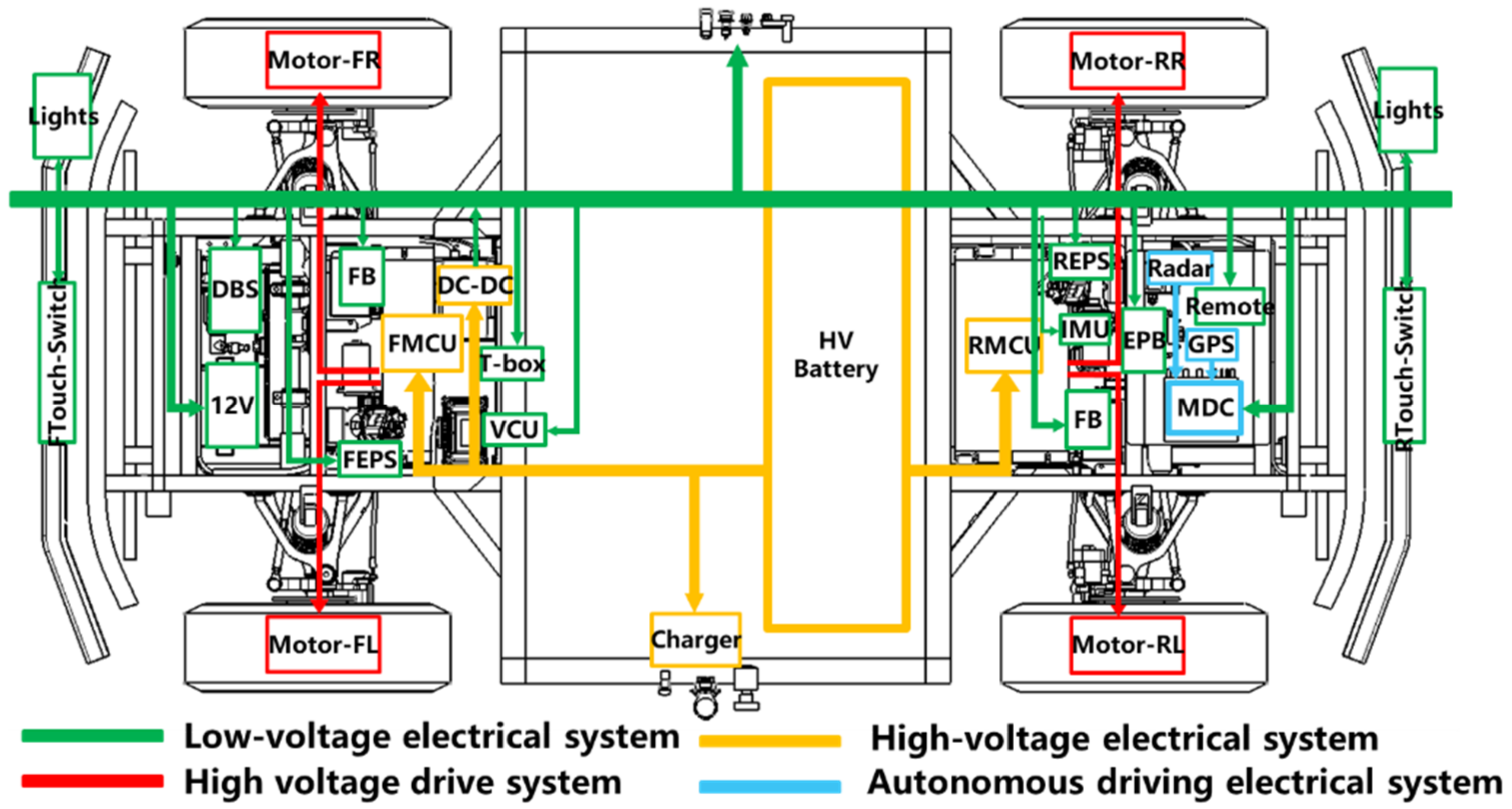
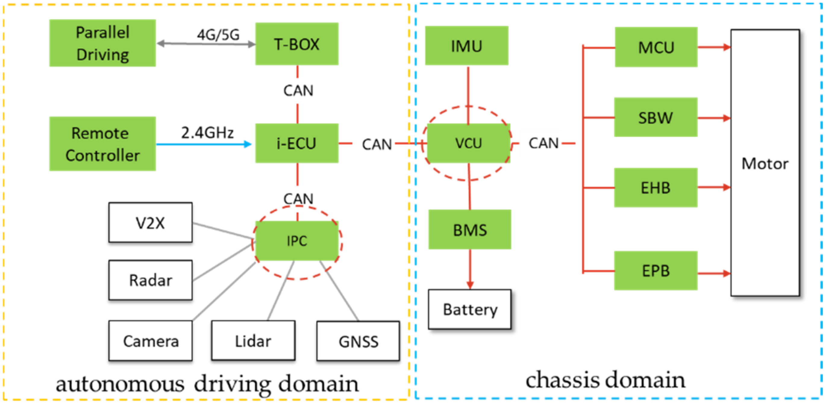
The electrical system for the four-wheel steer-by-wire chassis used in the experiment is as shown in Figure 4. The system has dual motors and two steer-by-wire modules to control the rotation and steering of front and rear wheels respectively. So, the 4WS vehicle has more freedom degrees used for attitude control. A combined positioning system uses Global Positioning System (GPS) and Inertial Navigation System (INS). The upper computer is used to monitor and collect data from the controller area network (CAN). All control algorithms code is downloaded to the ECU and run in the ECU.

The main structural parameters of 4WS AGV are shown in

Table 1. Vehicle parameters.

Parameters	Symbol	Value	Unit
The quality of the whole vehicle	$m$	700	kg
Wheelbase	$L$	1.9	m
Wheel track	$W$	1.2	m
Maximum steering angle	${\delta }_{\max }$	30	°/s
Maximum steering angle rate	$\Delta {\delta }_{\max }$	20	°/s

.

The vehicle drive control topology can be divided into the chassis domain and the autonomous driving domain as shown in Figure 5. The vehicle control unit (VCU) communicate with the motor control unit (MCU), the steering by wire (SBW), the electrical hydraulic brake (EHB), the electric park brake (EPB), the battery management system (BMS), and instrument electronic control unit (I-ECU) through the CAN bus to obtain the information of the remote control, the automatic driving domain computer (Industrial Personal Computer, IPC), and the parallel driving controller.

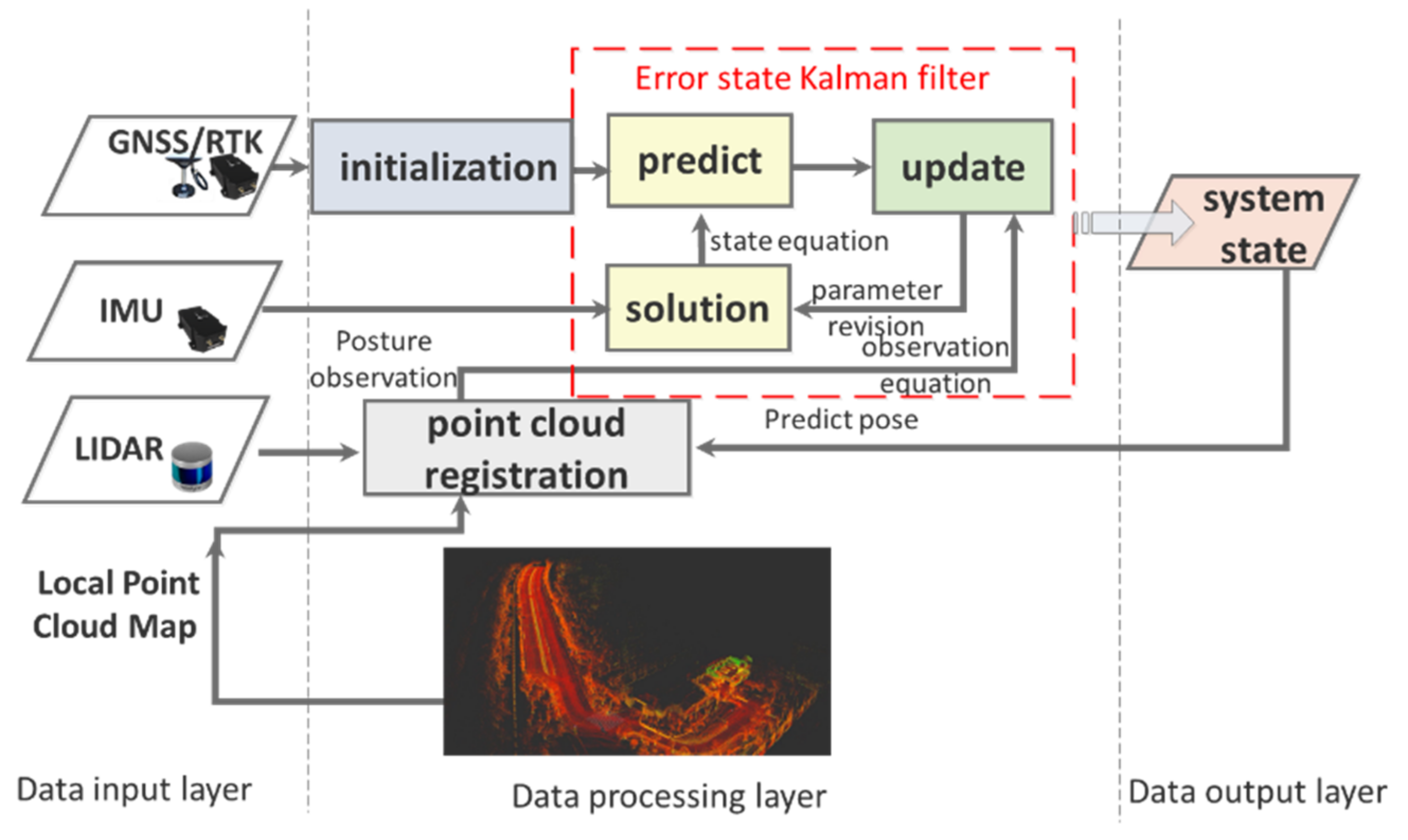
In the trajectory tracking control system established in this paper, lidar is mainly used to establish point cloud map and positioning. As shown in Figure 6, the acquisition of vehicle pose in this paper mainly relies on the fusion positioning system composed of lidar and GNSS-RTK.

When the vehicle starts outdoors, the navigation system is initialized with the GNSS-RTK information at the starting point. When the IMU data are received, the state variables of navigation system (position, speed, attitude, etc.) are updated recursively, and the recursive prediction is calculated to represent the uncertainty of the error state. When the LIDAR point cloud is received, the local map is used for registration, and the pose information of the vehicle relative to the local map is obtained. Taking the pose information as the observation, the new error state quantity and the filter gain are calculated. The parameters of the navigation module are modified according to the filter gain to realize the data fusion between IMU and LIDAR. As a result, vehicle pose is generated accurately and output to the control module.

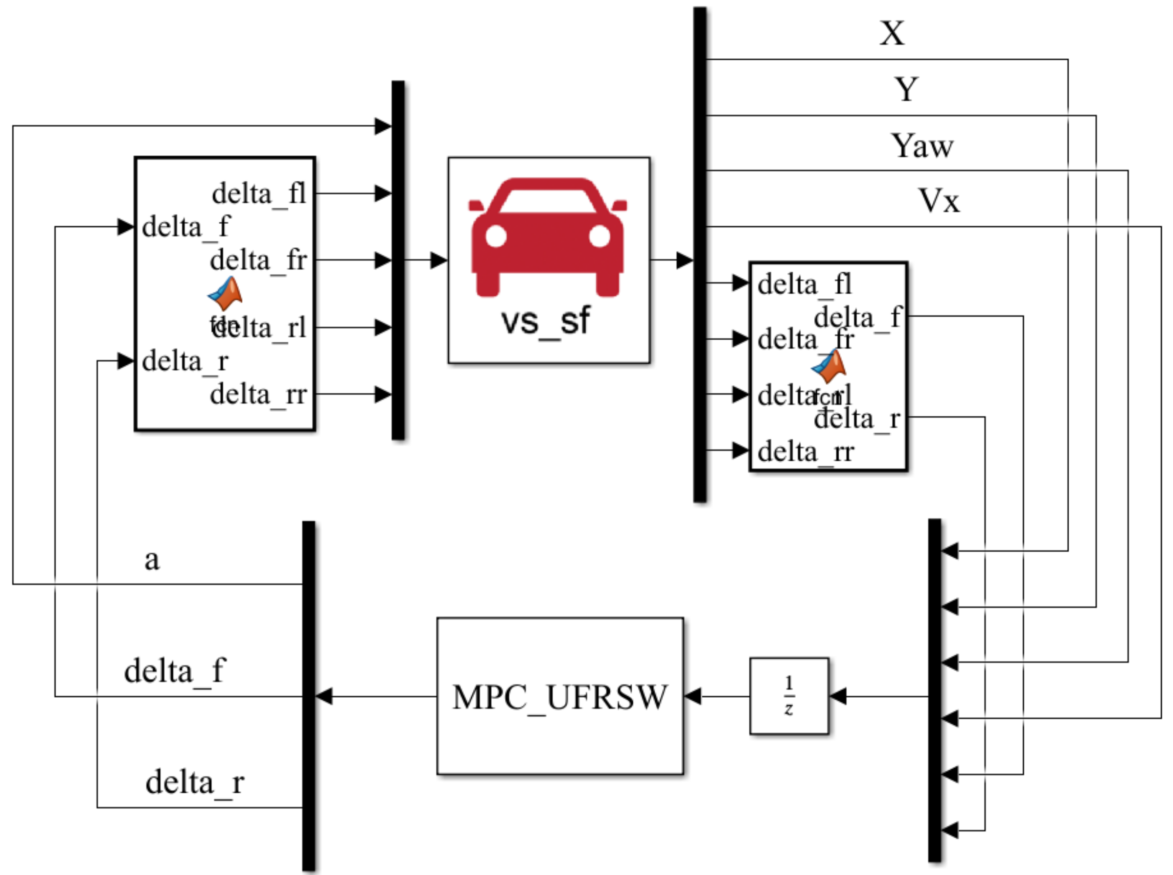
4.2. Simulation Platform Construction

Based on the vehicle parameters of the experimental platform, a vehicle dynamics simulation model is established in Carsim, where the road adhesion coefficient is set to 0.8, and the rolling resistance coefficient is set to 0.8. The trajectory tracking controller is built by the S-function module in Simulink. A co-simulation platform is established with Carsim as shown in Figure 7.

In the vehicle trajectory tracking simulation, the double lane change maneuver is a commonly used reference trajectory in the trajectory tracking test. In this paper, the function equation of the double lane change trajectory used in the simulation is as follows

$$\left\{\begin{array}{l}{Y}_{ref}(X)=\frac{d_{y1}}{2}(1+\tanh (z_1))-\frac{d_{y2}}{2}(1+\tanh (z_2))\\ {\phi }_{ref}(X)={\tan }^{-1}(d_{y1}{\left(\frac{1}{\cosh \left(z_1\right)}\right)}^2\left(\frac{1.2}{d_{x1}}\right)-d_{y2}{\left(\frac{1}{\cosh \left(z_2\right)}\right)}^2\left(\frac{1.2}{d_{x2}}\right))\end{array}\right.$$

(21)

where $z_1=\frac{2.4}{25}(X-27.19)-1.2$, $z_2=\frac{2.4}{21.95}(X-56.46)-1.2$, ${\mathrm{d}}_{\mathrm{x}1}= 25$, ${\mathrm{d}}_{\mathrm{x}2}= 21.95$, ${\mathrm{d}}_{\mathrm{y}1}= 4.05$, ${\mathrm{d}}_{\mathrm{y}2}= 5.7$.

4.3. Analysis of Simulation Results

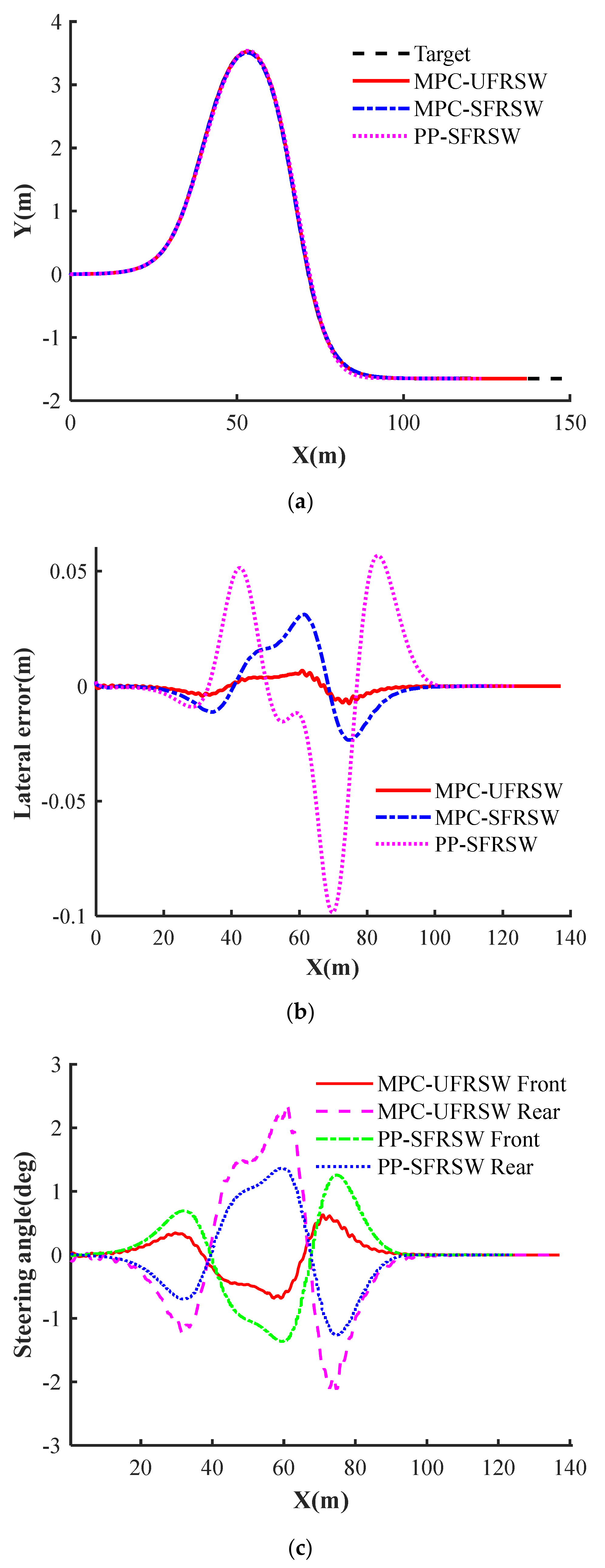
The simulation and real vehicle verification results are represented based on the trajectory of the vehicle’s geometric center point. As shown in Figure 8a,b, the MPC-UFRSS method has better tracking performance for double lane change maneuver. At a speed of 5 m/s, the maximum lateral tracking error of the MPC-UFRWS method does not exceed 0.01 m, with 0.03 m for the SFRSW method and 0.1 m for the PP-SFRSW method.

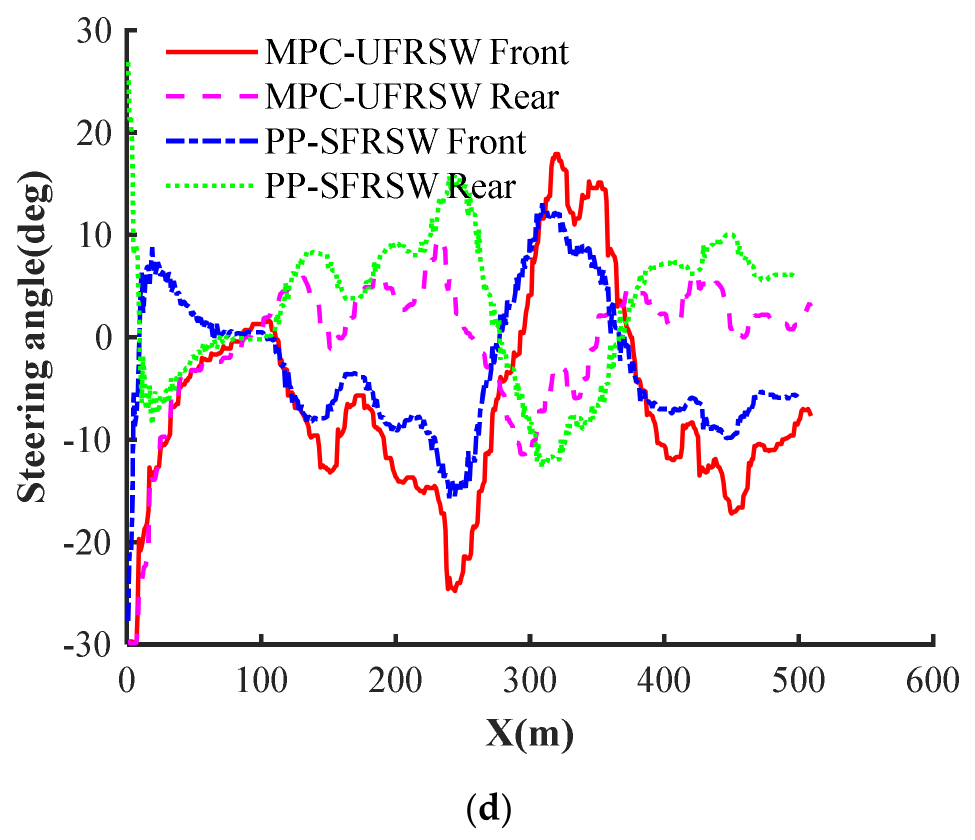
As shown in Figure 8c, the PP-SFRSW method has the hard constraint between the front and rear wheels that the equal steering angles and opposite phase, while the MPC-UFRWS does not have this limitation. Therefore, the latter steering control changes are more flexible in corners, and the front and rear wheels steering forms are more diverse. As shown in Figure 8, when the vehicle enters the curve, the MPC-UFRWS method is relatively gentle, while the lateral tracking error of the PP-SFRSW increases sharply. The front and rear wheels angle adjustment of the MPC-UFRWS is larger, which can respond to the change of tracking error faster and track reference trajectory more flexibly.

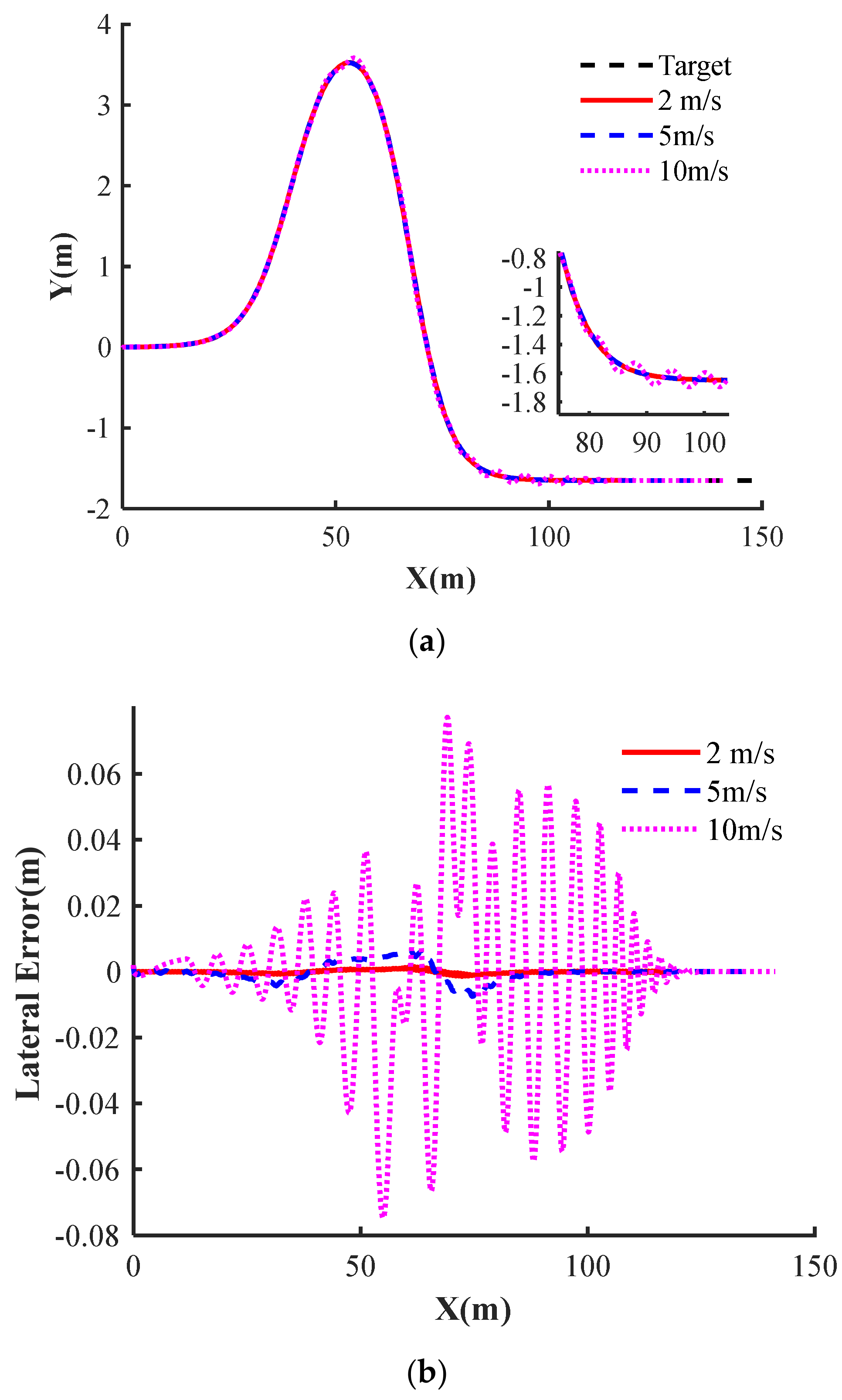
4.4. Simulation Comparison at Different Speeds

The trajectory tracking of the MPC-UFRWS method comparison at different speeds is as shown in Figure 9. The greater speed, the greater the control error and the greater the overshoot. Similar to other methods based on the kinematics model, the proposed method is suitable for low-speed conditions. When the speed is less than 5 m/s, the lateral tracking error is less than 0.01 m. When the speed is 10 m/s, the lateral tracking error is greater than 0.06 m. However, when the speed is 15 m/s, the vehicle path deviates far from the reference path.

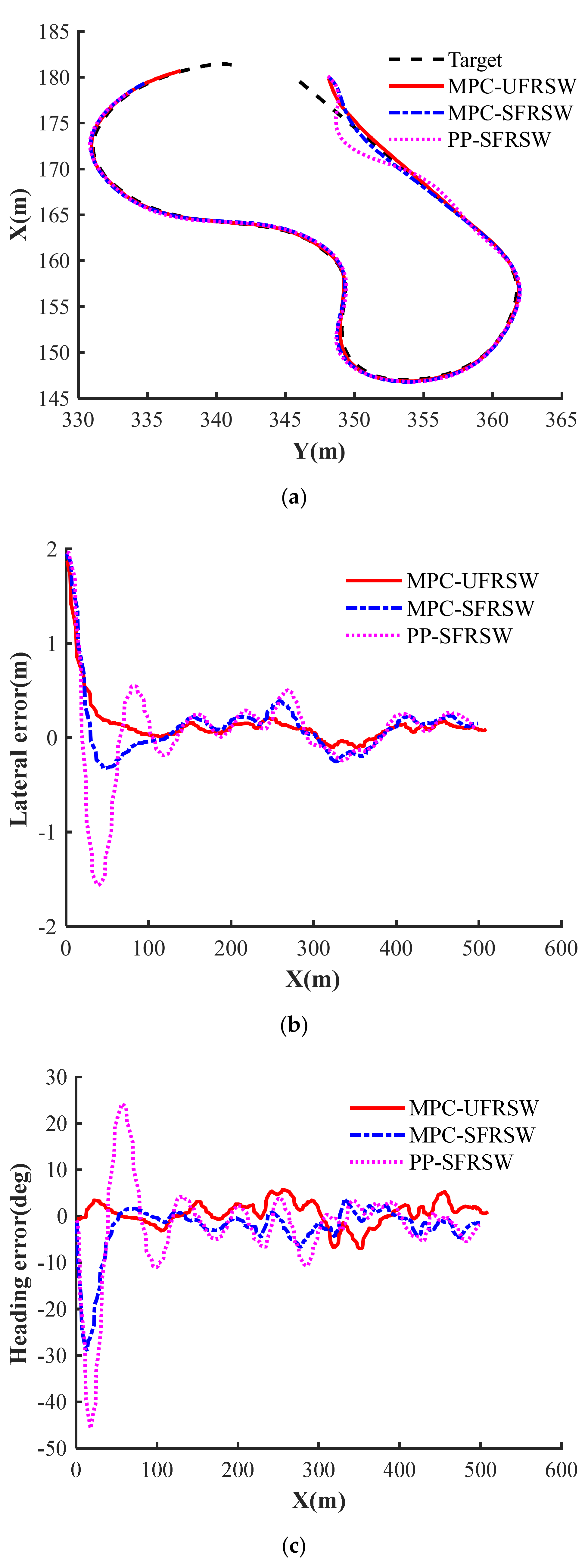
4.5. Analysis of Real Vehicle Verification Results

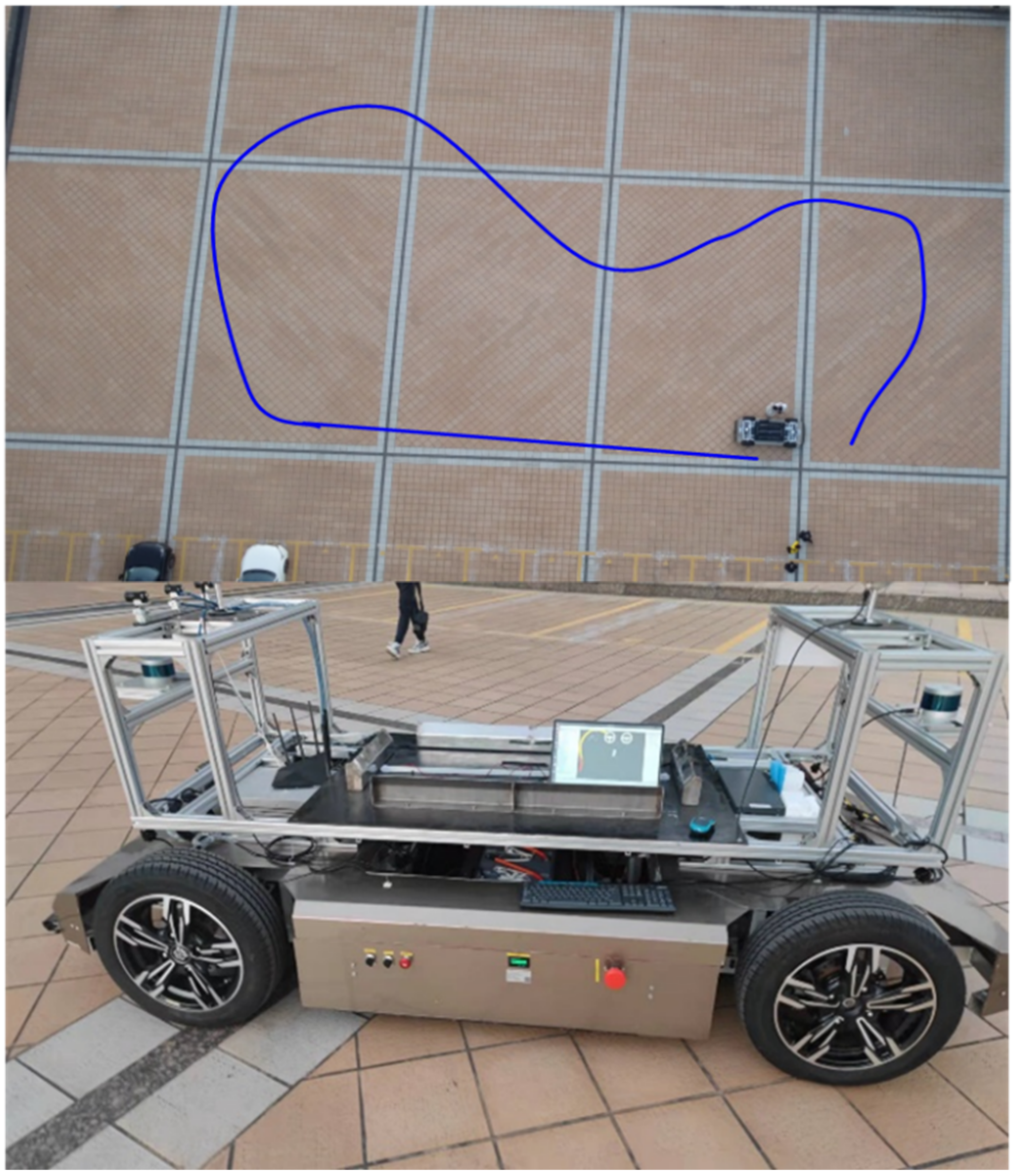
To ensure the safety of personnel and vehicles, the vehicle experiment was carried out in an open space of Sun Yat-sen University. To verify the performance of the vehicle tracking straight and curved lines at the same time, we choose a recorded B-like trajectory as the reference trajectory considering the site constraints. The test site and vehicle are as shown in Figure 10.

The real vehicle verification results of MPC-UFRWS, PP-SFRWS, and MPC-SFRWS are as shown in Figure 11 and

Table 2. Result data of vehicle verification.

Method	Max LatErr	MaxYawErr	stdPLatErr	stdPYawErr
PP-SFRWS	0.7663	12.2829	0.3168	3.4911
MPC-SFRWS	0.3488	7.2850	0.1202	1.7169
MPC-UFRWS	0.1998	6.7354	0.0678	2.6064

, and analysis are as follows:

• Compared with the PP-SFRWS method, the trajectory tracking accuracy of the MPC-UFRSW is higher. At the speed of 2 m/s, the maximum lateral error and yaw angle error are reduced by 0.567 m and 5.55°, respectively. This is because the Pure Pursuit method only determines the control input based on the deviation of the current measured values from the reference value, while the MPC method uses the prediction model to estimate the future deviation value and determine the current values in a rolling optimization manner.
• The MPC-UFRWS method has higher tracking accuracy than the MPC-SRFRS. At a speed of 2 m/s, the maximum lateral error and yaw angle error are reduced by 0.15 m and 0.5°, respectively. This is because MPC-UFRWS does not constrain the relationship between the front and rear wheels angle, which can give full play to the more flexible characteristics of 4WS vehicle and avoid oversteering or understeering.
• The proposed method enables better steering flexibility of 4WS vehicle. At the starting point, the lateral error between the vehicle and the reference trajectory is about 2.5 m. When the vehicle starts to drive, the MPC-URFSW method makes the vehicle merge into the trajectory in an approximate crab-walking manner, while the front and rear wheels turn in phase or out of phase in the corners. Therefore, the proposed method can realize the switching of various steering modes such as out-of-phase steering and crab steering without adding additional judgment.
• Compared with the simulation results, the real vehicle tracking error increases several times. The reason may be that the curvature change rate of the B-like rail is larger than the double lane change maneuver. At the same time, external factors such as actuators, sensors, and road surfaces may also cause large tracking errors during vehicle verification.

5. Conclusions

In this paper, a path tracking controller with unconstrained front and rear wheels steering is established for the trajectory tracking control of 4WS vehicle. The controller relies on the proposed optimization function considering the tracking accuracy and control flexibility. Then, the simulation and vehicle verification are carried out to prove the effectiveness of the controller. In the Carsim/Simulink platform, MPC-UFRSW has higher tracking accuracy than PP-SFRSW and MPC-SFRSW when tracking double lane change trajectory at a speed not exceeding 10 m/s. In the real vehicle experiment with B-like curve, the steering angle of the front and rear wheels of the proposed controller changes more flexibly. The maximum lateral error and yaw angle error are reduced by 60% and 9%, respectively. The simulation and real vehicle verification results show that the proposed method has more flexible steering modes and higher tracking accuracy. The next work will further analyze the stability of the trajectory tracking of the 4WS vehicle at high speed from the dynamic point of view.