Experimental Study of Dynamical Airfoil and Aerodynamic Prediction

Abstract

Dynamic stall is a critical limiting factor for airfoil aerodynamics and a challenging problem for active flow control. In this experimental study, dynamic stall was measured by high-frequency surface pressure tapes and pressure-sensitive paint (PSP). The influence of the oscillation frequency was examined. Dynamic mode decomposition (DMD) with time-delay embedding was proposed to predict the pressure field on the oscillating airfoil based on scattered pressure measurements. DMD with time-delay embedding was able to reconstruct and predict the dynamic stall based on scattered measurements with much higher accuracy than standard DMD. The reconstruction accuracy of this method increased with the number of delay steps, but this also prolonged the computation time. In summary, using the Koopman operator obtained by DMD with time-delay embedding, the future dynamic pressure on an oscillating airfoil can be accurately predicted. This method provides powerful support for active flow control of dynamic stall.

1. Introduction

Stall is one of the most critical limiting factors for airfoil aerodynamics. Static stall occurs when the airfoil reaches a certain angle of attack. However, in real-world applications, dynamic stall caused by an unsteady motion is more common. An example of such motion is the rapid pitch-up of the airfoil in rotor blades and wind turbines. Compared with static stall, dynamic stall is a more complicated unsteady phenomenon due to the flow separation caused by the rapid change in the angle of attack and the variable stall frequency. Thus, it leads to an abrupt decay of aerodynamic forces and a fluctuation of the structural load on the airfoil. McCroskey et al. [1] comprehensively studied dynamic stall in an oscillating airfoil and dynamic vortex shedding from the airfoil. Further research [2,3,4,5] has since provided a detailed understanding of the characteristics of dynamic stall with respect to the lift and pitch moment coefficient. Carr et al. [6] reviewed the significant progress in dynamic stall and concluded that the key influencing factors of this process were oscillation amplitude and frequency, Mach number, and the three-dimensional effects of the airfoil.

Dynamic stall is common in practical engineering and detrimental to the performance of air vehicles. Many researchers employed vortex generators to realize effective control of the dynamic stall [7,8]. Vortex generator control is a passive control method, which is easy-implemented and does not require extra energy injection. However, passive control cannot adapt to the change in working conditions. Recently, many researchers focused on active flow control, which is adjustable based on a feedback control loop [9,10,11,12]. Therefore, real-time sensing of the complicated and unsteady flow, e.g., the dynamic stall, is critical in the control loop.

The use of pressure tapes for local measurements is considered a promising method to investigate the flow conditions on an airfoil due to their reliability and ease of implementation. To reduce the complexity of the algorithm or system, some researchers applied some conventional and easy-implemented methods to identify the aerodynamic parameters of the airfoils. Therefore, it is important to predict the flow dynamic based on scattered pressure data. Patel et al. [13] used a pressure sensor array on the upper surface of an airfoil to detect the onset of flow separation. Saini et al. [14] predicted the aerodynamic parameters (i.e., inflow velocity and angle of attack) using discrete surface pressures measured at ports in the vicinity of the leading edge of an airfoil. Provost et al. [15] used a time-shift linear model to predict the roll moment using a sparse set of surface pressure measurements. Juliano et al. [16] found that the pressure field on an oscillating airfoil can have distinct patterns at different locations that are difficult to capture using pressure sensors. Similarly, An et al. [17] develop a method for estimating the instantaneous lift coefficient on a rapidly pitching airfoil that uses a small number of pressure sensors and a measurement of the angle of attack. Gao et al. [18] detected unsteady boundary layer transition on a pitching airfoil using a statistical criterion calculated from thirty surface-pressure transducer measurements. With the development of artificial intelligence, the machine learning method has been successfully applied to sense or predict the aerodynamic parameters [19,20]. However, machine learning methods, such as a blacked box, cannot provide an interpretable physical explanation. Therefore, some researchers employed data-driven techniques to realize the system or parameters identification [21,22,23]. Zhou et al. [24] explained the physical relationship of pressure data and then developed an offline-online method to sense the real-time aerodynamic parameters. Saini et al. [25] developed the leading-edge flow sensing technique, which uses a few pressures in the airfoil leading-edge to identify and sense various flow events associated with vortex shedding in unsteady airfoils.

Most of the researches mentioned above focused on the flow field around static objects. The associated and available methods typically combine proper orthogonal decomposition (POD) with other algorithms, such as linear stochastic estimation [26] and particle filter [27]. However, it is difficult to predict the evolution of the aerodynamics of dynamic airfoil over time. In this regard, the dynamical system concept should be taken into consideration, and dynamic mode decomposition (DMD) can provide some inspiration, which is an equation-free and data-driven method to model dynamical systems. DMD was initially proposed by Schmid [28] to decompose the flow field into both spatially and temporally coherent structures and has the capability of predicting dynamic systems in the temporal domain. Berger et al. [29] successfully applied DMD to control robotic movement parameters by predicting human–robot interactions based on initial-state input data. However, it is difficult for standard DMD to make predictions based on scattered measurements because the method relies on an infinite-dimensional linear dynamic approximation for a finite-dimensional nonlinear dynamic system. It, therefore, may not provide an accurate result or may even fail when applied to highly nonlinear systems with low-dimensional measurement data [30]. To solve this problem, some data-driven methods have been proposed. The theory of DMD with delay embedding was proposed by Brunton et al. [31] to decompose a three-dimensional chaotic Lorenz system into a linear model in the delay coordinates using a single variable. Mohammad et al. [32] utilized DMD in time delay coordinates to capture the dynamics of a compressible signal containing oscillation perfectly. In addition, Susuki et al. [33] conducted this method to realize the prediction of the voltage dynamics of the rudimentary model directly from the single-bus measurement. The time delay embedding [34] has been investigated in detail on the structure and conditioning of linear models of nonlinear dynamics. Yuan et al. [35] developed DMD with a delay embedding method to predict high temporal and spatial resolved flow fields based on local particle image velocimetry (PIV) measurement. Arbabi et al. [36] applied the delay embedding method to sparse measurements and realized predictive control of nonlinear flow based on a Koopman model framework.

In the current work, the scattered data obtained from pressure tapes on the surface of an airfoil were used to predict the surface pressure of the airfoil during the oscillation process. Pressure-sensitive paint (PSP) surface measurement provided a qualitative visualization to verify the dynamic stall on the oscillating airfoil. Based on the scattered pressure tape measurements, DMD with time-delay embedding was applied to reconstruct the spatiotemporal pressure distribution on the oscillating airfoil and predict the future data in real-time.

2. Experimental Setup and Methodology

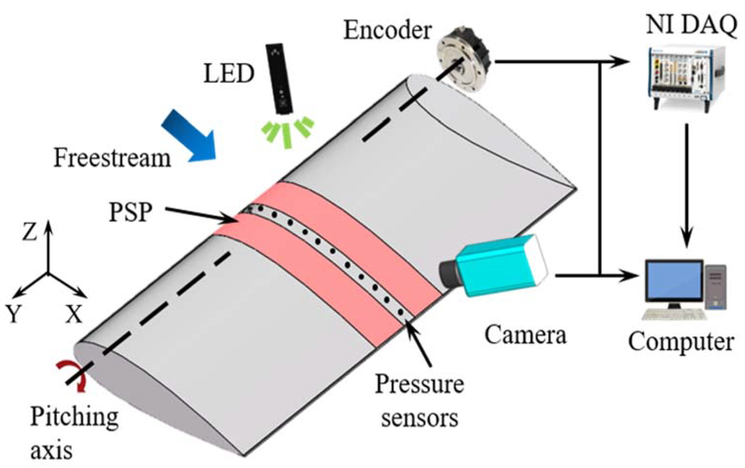
2.1. Measurement Setup

The experiment was conducted in an open-circuit low-speed wind tunnel at the China Aerodynamics Research and Development Center. The test section of the wind tunnel has a cross-section of 1.8 m × 1.4 m. In the experiment, the freestream velocity was U_∞ = 34 m/s. The two-dimensional airfoil model OA309, made of high-strength carbon fiber composite materials, with a chord length of c = 0.4 m and span length of s = 1.8 m, was mounted on a pitching testing platform. The freestream Reynolds number based on the chord length c was Re = 0.9 × 10⁶. The airfoil model was subjected to an unsteady periodic motion. As shown in Figure 1, the pitching motion mechanism was composed of a servo motor, planetary reducer, and encoder. The mechanism allowed control over motion parameters, such as mean angle of attack α₀, pitching amplitude α₁, and oscillation frequency f. In the experiment, α₀ was set as 10°, α₁ was set as 10°, and f was varied as 1, 2, 3, and 4 Hz. The reduced frequency was defined as k = πfc/U_∞, with values of 0.037, 0.074, 0.111, and 0.148. The formula for the angle of attack α can be expressed as follows:

$$\alpha ={\alpha }_0+{\alpha }_{1}sin\left(2\pi ft\right)$$

(1)

The PSP measurement system and pressure tapes are shown in Figure 1. Part of the upper surface of the airfoil was painted with PSP to evaluate the changes in pressure distribution when the airfoil was oscillating. The PSP was excited by a UV LED (UHP-T-385-EP from Prizmatix Ltd., Givat Shmuel, Israel), and images were captured by a camera (PCO 1600) with a filter. Using a synchronizer (BNC-575) and potentiometer, PSP images were captured during certain phases of the oscillating airfoil. During the PSP measurement process, exposure signals from the camera were acquired simultaneously with measurements from the potentiometer, which contained the angle of attack of the airfoil. Using these two signals, every PSP frame was assigned to a certain angle of attack. Then, the phase-locked pressure distribution of the upper surface of the airfoil could be obtained by PSP measurement.

The pressure tape measurements and PSP measurements were taken simultaneously. Forty dynamic differential pressure sensors (8510B, ENDVECO) were arranged chordwise at the midspan of the airfoil model. The measurement range of these pressure sensors is 1 psi, and the measurement inaccuracy is ±0.05% of full scale. Locations of these 40 pressure sensors are detailed in

Table 1. Locations of the pressure transducers on the OA209 airfoil.

Upper Surface				Lower Surface
No.	x/c	No.	x/c	No.	x/c	No.	x/c
1	0.01	11	0.24	21	0	31	0.25
2	0.02	12	0.3	22	0.0125	32	0.3
3	0.03	13	0.36	23	0.025	33	0.35
4	0.04	14	0.42	24	0.0375	34	0.4
5	0.05	15	0.48	25	0.05	35	0.5
6	0.06	16	0.57	26	0.075	36	0.6
7	0.09	17	0.66	27	0.1	37	0.7
8	0.12	18	0.75	28	0.125	38	0.8
9	0.15	19	0.84	29	0.15	39	0.9
10	0.18	20	0.93	30	0.2	40	1

. These pressure sensors adopted a dynamic sampling frequency to sample 256 data points per oscillation cycle of the dynamic airfoil. The acquisition time was approximately 30 s. The aerodynamic parameters, such as lift and pitching moments, were obtained by the integration of the pressure data. Aerodynamic loads can be calculated based on the integration of the surface pressure coefficient. The pressure coefficients can be calculated from the following expression:

$$C_{p_i}=\frac{P_i-P_{\infty }}{\frac{1}{2}\rho U_{\infty }}$$

(2)

where ρ is the air density, P_i is the static pressure obtained from a single pressure tap, P_∞ is the static pressure of the incoming flow. The detailed process of the integration can refer to previous material [37].

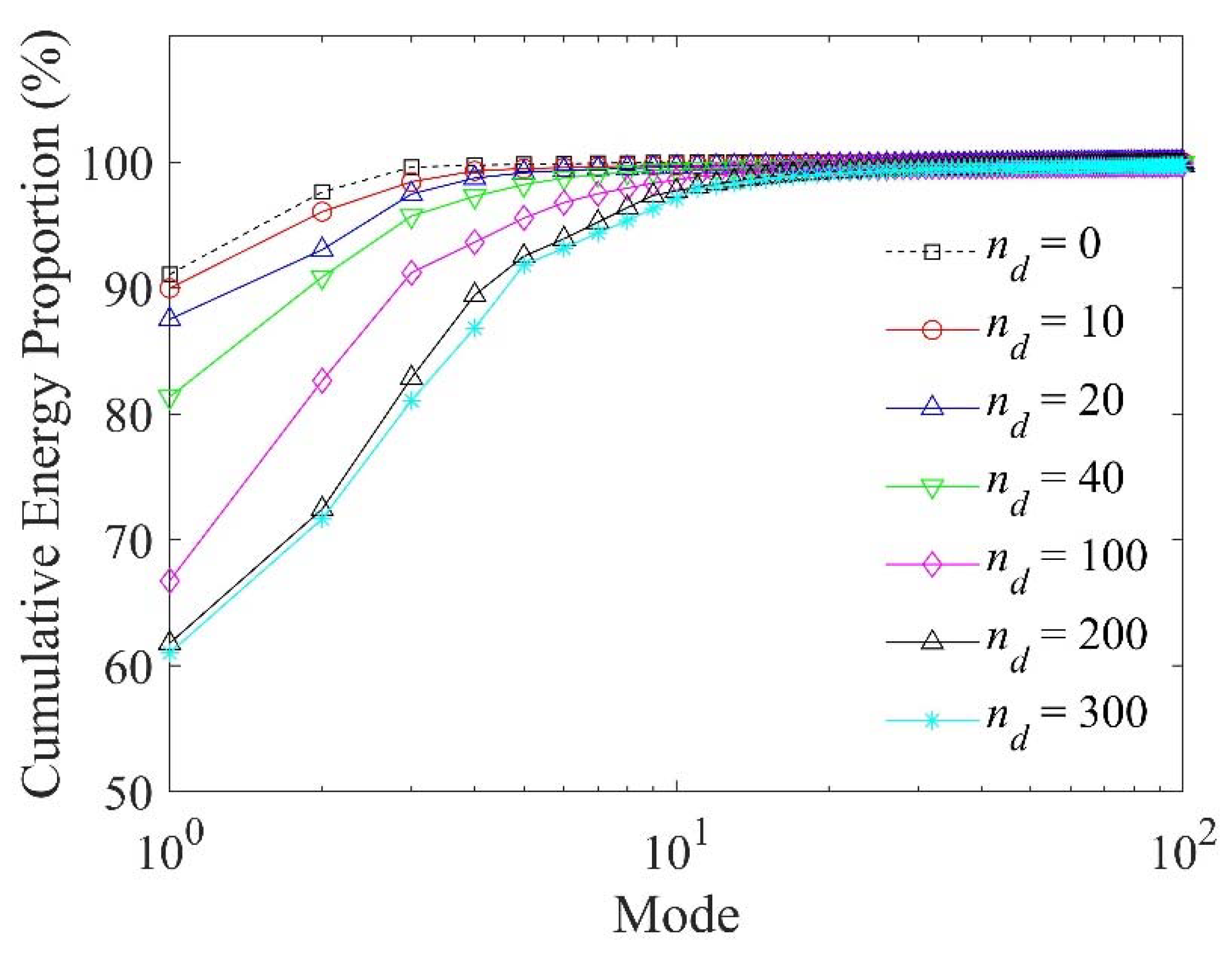
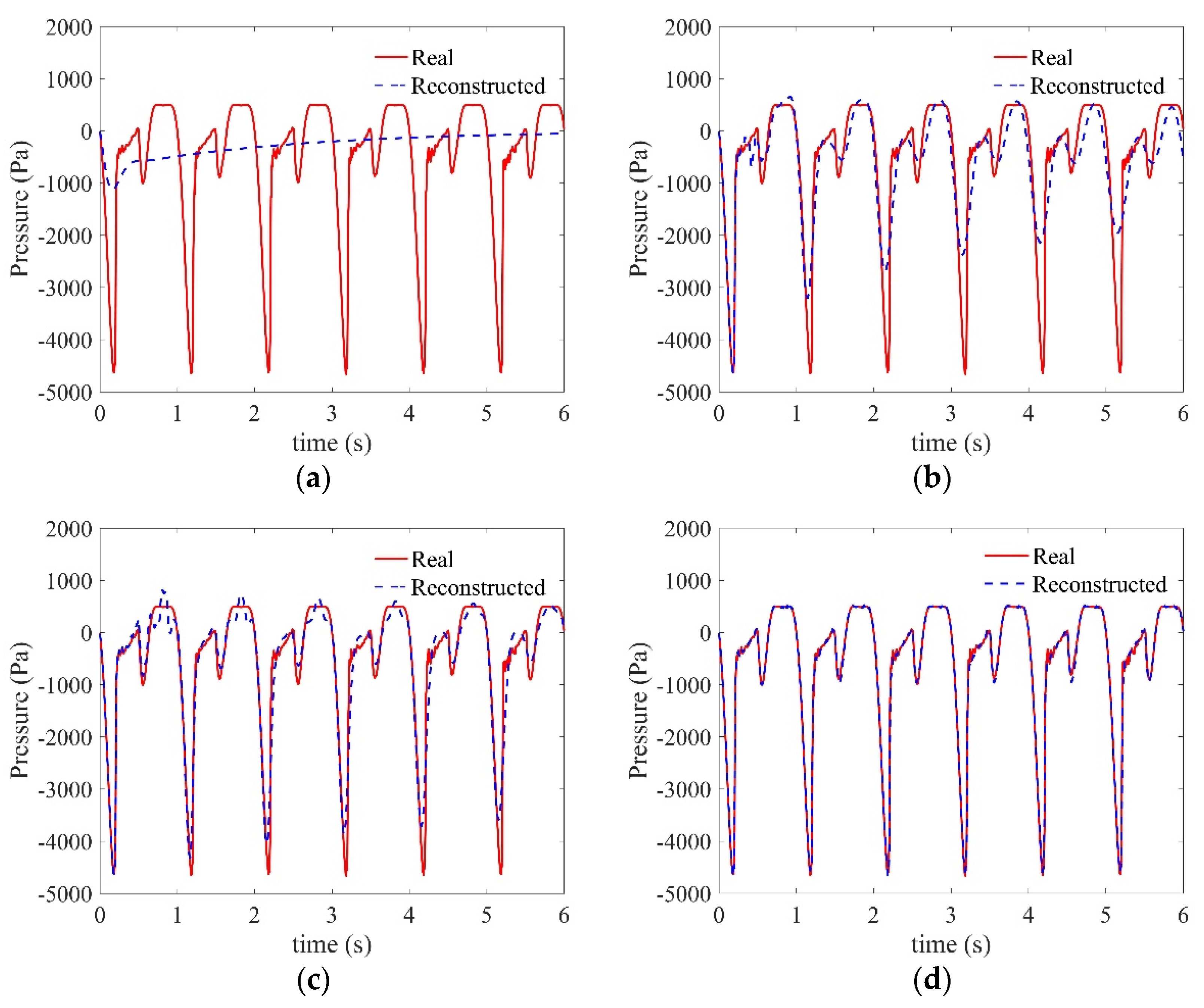
2.2. Dynamic Mode Decomposition with Time-Delay Embedding

DMD is an efficient method of decomposing a dynamical system into specific spatial modes that evolve at a certain frequency and growth–decay rate in time. In DMD, the measurement data obtained by sensors at time j are arranged into a column vector x_j = (x_1,j, x_2,j,…, x_n,j), where x_j is a data snapshot and n denotes the number of measurement points (in this case, the number of sensors). All m snapshots were sampled with a constant time interval (sampling time step) Δt. DMD describes a discrete-time system as:

x_j+1 = Ax_j

(3)

where matrix A reflects the dynamical characteristics of the system. The first step of DMD is to arrange all m snapshots into two matrices, X₁ = (x₁, x₂, …, x_m−1) and X₂ = (x₂, x₃, …, x_m). Then, the linear approximation A may be written in terms of matrices based on Equation (4) as:

X₂ ≈ AX₁

(4)

Using matrix A, known as the Koopman operator, future data can be predicted from current data. Thus, the core of DMD is to search for the optimal linear approximation A of the nonlinear dynamical system. The crucial step of the DMD algorithm is obtaining the rank-reduced representation of A in terms of a POD-projected matrix $\tilde{A}$, which can be written as follows:

$$\tilde{A}=U^{\mathrm{T}}AU=U^{\mathrm{T}}{X}_{2}V{\Sigma }^{-1}$$

(5)

where U ∈ R^n×r, Σ ∈ R^r×r, and V ∈ R^m×r are obtained by singular value decomposition (SVD). Here, r is defined as the truncated number and represents the rank of approximation to X₁ using SVD reduction. The next step is to compute the eigen-decomposition of $\tilde{A}$, which is similar to A:

$$\tilde{A}W=W\Lambda$$

(6)

where the columns of W are eigenvectors of $\tilde{A}$ and Λ is a diagonal matrix containing the eigenvalues λ_k, which capture the time dynamics of the corresponding DMD modes. These eigenvalues and eigenvectors of $\tilde{A}$ can be related back to the similarity-transformed eigenvalues and eigenvectors of A to reconstruct the DMD modes given by:

$$\Phi =X_{2}V{\Sigma }^{-1}W$$

(7)

where $\Phi$ is the matrix whose columns each represent a DMD mode. Then, a snapshot at any time can be reconstructed from the DMD modes and eigenvalues:

x_j = ΦΣ^j−1b

(8)

where b = Φ^−1 × ₁ contains the initial values of DMD modes. As shown above, the DMD method relies on the linear approximation of a nonlinear dynamic system. When the sub-domains are of limited spatial dimensionality, it is difficult for DMD to provide accurate predictions. In this study, the direct use of discrete sensor measurements as the observables creates a system that is far removed from the infinite-dimensional linear approximation of highly nonlinear systems. To solve this problem, extended DMD [38] and kernel DMD [39] have previously been proposed. These methods use new observables to provide a set of coordinates in which the dynamical systems appear linear. However, a universal and systematic approach needs to be found. The details of time delay embedding methods can refer to the works of Brunton et al. [31]. Time-delay embedding augments the limited spatial observables by embedding future measurements into the current measurements. Therefore, more information can be captured to construct the linear Koopman operator.

A requirement of time-delay embedding is to have access to at least n_d + 1 consecutive snapshots, where n_d is the number of delay steps. The time-delay-embedded matrices X₁ and X₂ can be transformed into H₁ and H₂ as follows:

$${\mathit{H}}_{\mathbf{1}}=\left[\begin{array}{cccc}{\mathit{x}}_{\mathbf{1}}& {\mathit{x}}_{\mathbf{2}}& \mathbf{\cdots }& {\mathit{x}}_{\mathit{m}-{\mathit{n}}_{\mathit{d}}}\\ {\mathit{x}}_{\mathbf{2}}& {\mathit{x}}_{\mathbf{3}}& \mathbf{\dots }& {\mathit{x}}_{\mathit{m}-{\mathit{n}}_{\mathit{d}}+\mathbf{1}}\\ \mathbf{⋮}& \mathbf{⋮}& \mathbf{\ddots }& \mathbf{⋮}\\ {\mathit{x}}_{{\mathit{n}}_{\mathit{d}}}& {\mathit{x}}_{{\mathit{n}}_{\mathit{d}}+\mathbf{1}}& \mathbf{\cdots }& {\mathit{x}}_{\mathit{m}-\mathbf{1}}\end{array}\right]=\left[y_1,y_2\cdots y_{m-n_d}\right],$$

(9)

$${\mathit{H}}_{\mathbf{2}}=\left[\begin{array}{cccc}{\mathit{x}}_{\mathbf{2}}& {\mathit{x}}_{\mathbf{3}}& \mathbf{\cdots }& {\mathit{x}}_{\mathit{m}-{\mathit{n}}_{\mathit{d}}+\mathbf{1}}\\ {\mathit{x}}_{\mathbf{3}}& {\mathit{x}}_{\mathbf{4}}& \mathbf{\dots }& {\mathit{x}}_{\mathit{m}-{\mathit{n}}_{\mathit{d}}+\mathbf{2}}\\ \mathbf{⋮}& \mathbf{⋮}& \mathbf{\ddots }& \mathbf{⋮}\\ {\mathit{x}}_{{\mathit{n}}_{\mathit{d}}+\mathbf{1}}& {\mathit{x}}_{{\mathit{n}}_{\mathit{d}}+\mathbf{2}}& \mathbf{\cdots }& {\mathit{x}}_{\mathit{m}}\end{array}\right]=\left[y_2,y_3\cdots y_{m-n_d+1}\right],$$

(10)

where $y_j$ is a new snapshot after delay embedding, and ${\mathit{x}}_{\mathit{m}}$ occupies the last n rows $y_{m-n_d+1}$.

The dimensions of the matrices after delay embedding H₁ and H₂, are $(n\times n_{d)}\times \left(m-n_d\right)$. When n_d = 1, the matrix after delay embedding is the same as the original matrix. Analogously to Equation (4), the linear mapping of H₁ and H₂ can be written as follows:

H₂ ≈ BH₁

(11)

Then, the time-delay-embedded matrices H₁ and H₂ are used to build the DMD model. The matrix B is the Koopman operator and reflects the dynamical characteristics. Therefore, standard DMD can be applied to find the corresponding eigenvalues and eigenvectors of B. Using the matrix B as follows:

$$y_{j+1}\approx B{y}_j$$

(12)

The current new snapshot $y_j$ at time $n_d+j-1$ can be used to predict the future new snapshot $y_{j+1}$, which contains the data at time $n_d+j$.

3. Results and Discussion

3.1. Dynamic Stall

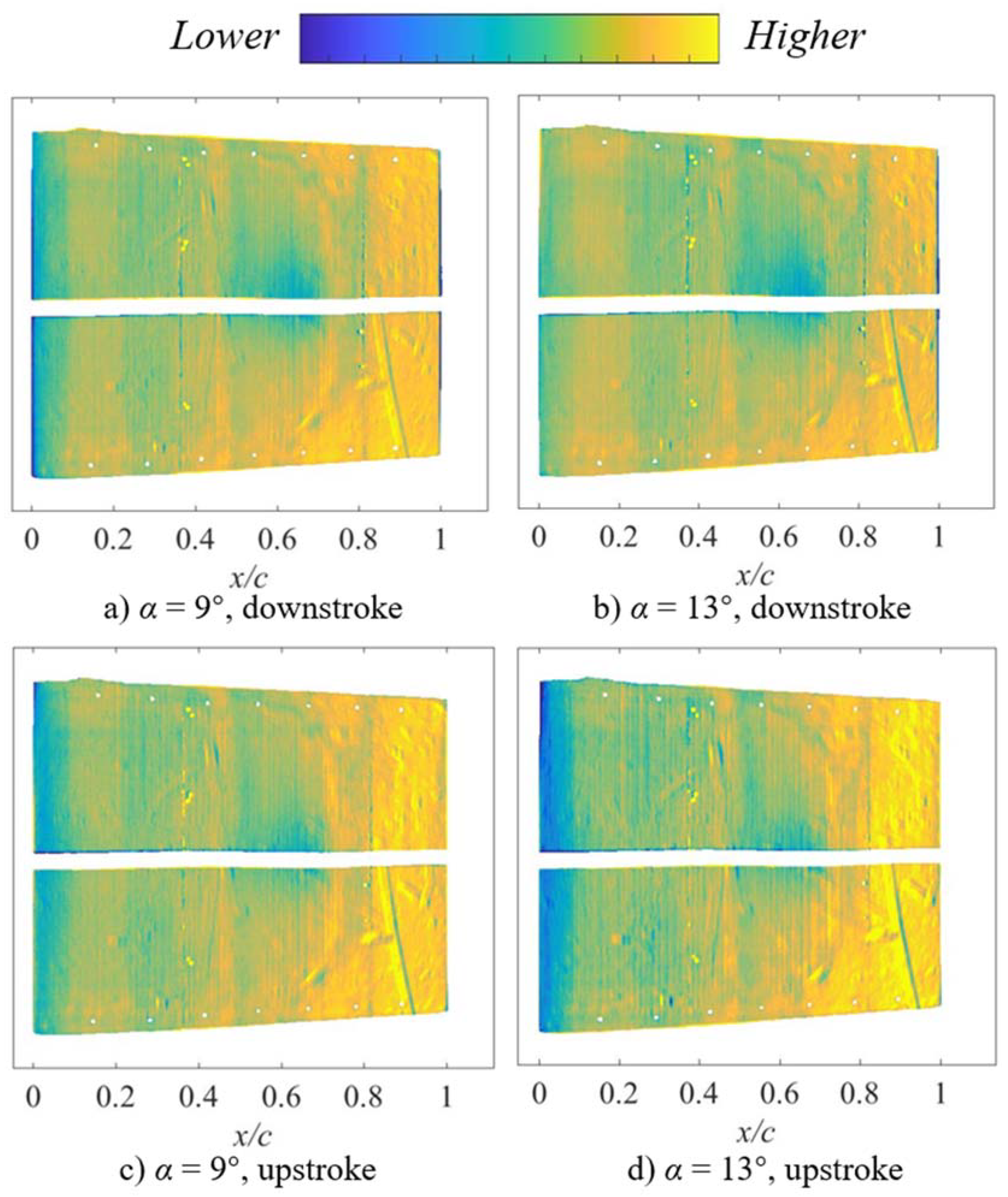
3.1.1. Flow Visualization

To examine the two-dimensional pressure field on the oscillating airfoil, the images from PSP measurement were phase-averaged over 15 periods. The evolution of the pressure field during the oscillation of the clean airfoil is shown in Figure 2 at two typical AoAs under an oscillation frequency of f = 1 Hz. It should be noted that these PSP measurements only provided a qualitative visualization because the PSP data was influenced by the temperature of the incoming flow.

The upper panels represent the downstroke, and the lower panels represent the upstroke. The low-pressure region is indicated in blue, and high pressures are shown in yellow. At α = 9°, the pressure distribution in the downstroke is similar to that in the upstroke. However, when α increases to 13°, an obvious low-pressure region forms at the leading edge of the airfoil in the upstroke, as can be seen in Figure 2d. The color intensity shows that the pressure at the leading edge in the downstroke is higher than that in the upstroke at the same angle of attack, which suggests the onset of flow separation and the decrease in lift. The phenomenon that flow separation occurs at the leading edge in the downstroke but does not occur in the upstroke is consistent with the dynamic stall was also investigated by Heine et al. using PIV measurement [8].

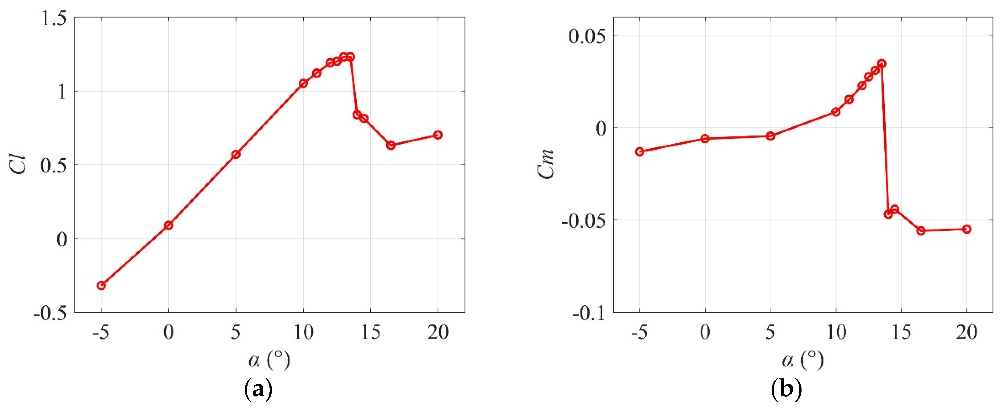
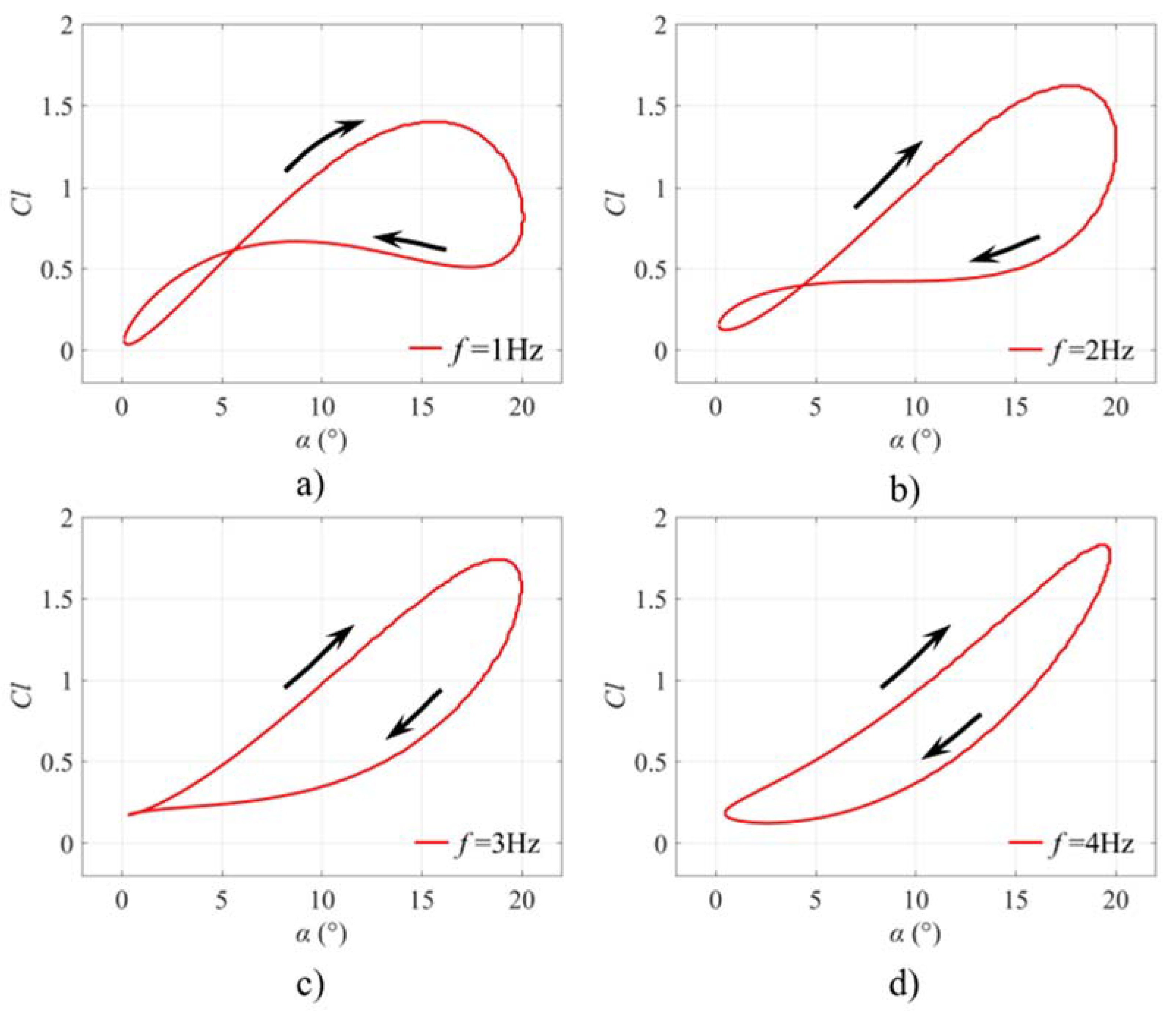
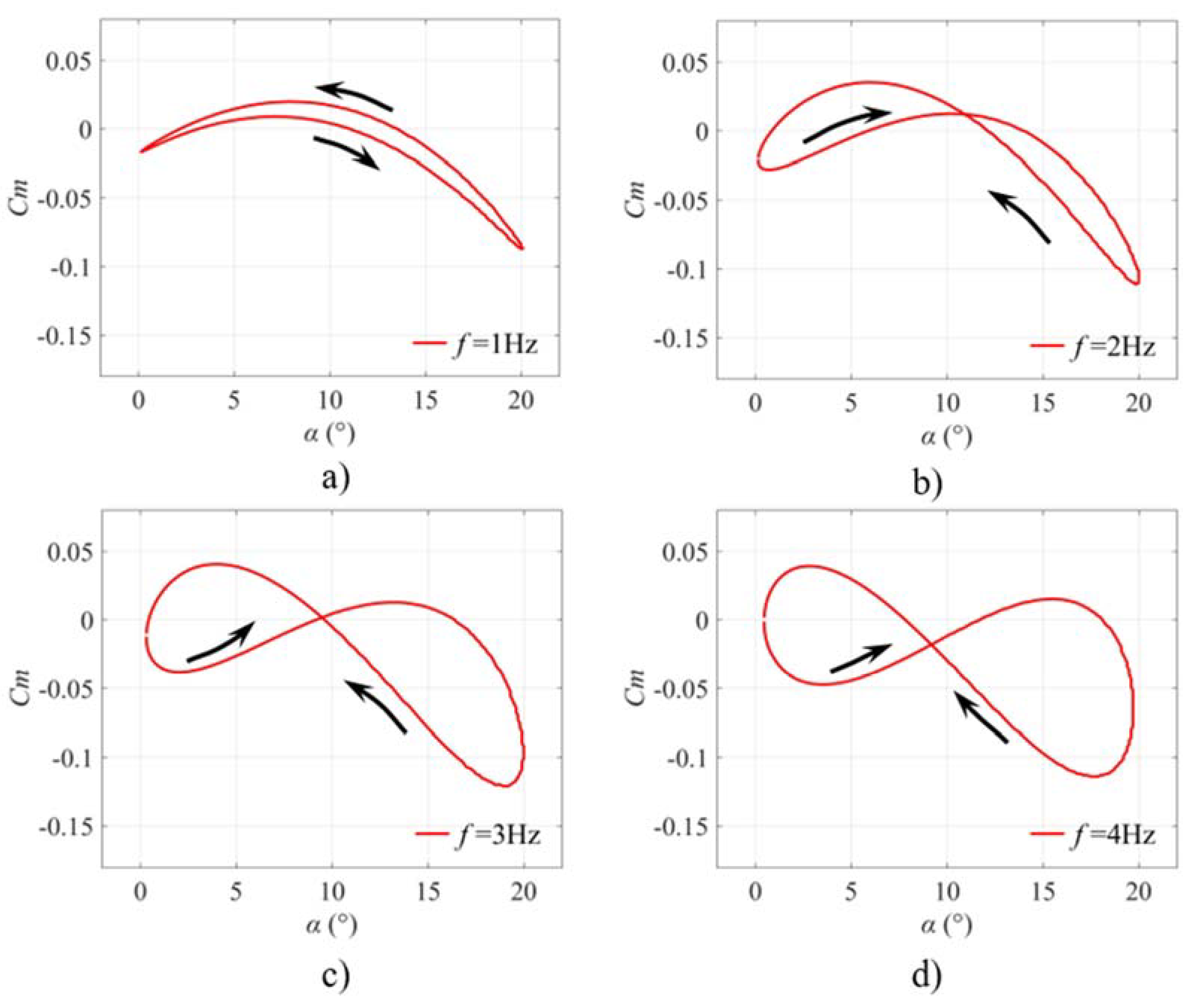
3.1.2. Aerodynamic Loads

The angle of attack of the airfoil was varied to examine the influence of the VGs mounted at the leading edge of the airfoil on the static aerodynamic loads. In our study, the aerodynamic loads of static and dynamical airfoil were measured to verify the phenomenon of dynamic stall. The measurement results of static airfoil are shown in Figure 3. Note that there is no oscillation frequency for this static case. As shown in Figure 3, the curves of the lift and pitch moment show a relatively constant trend until α ≈ 13.5°. With a further increase in the angle of attack, the lift and pitch moment drop abruptly. An increase of 0.5° in the angle of attack leads to a drop of approximately 0.39 in the lift coefficient and 0.08 in the pitch moment coefficient. Therefore, α = 13.5° can be considered as the stall angle with respect to flow separation. These results were in line with our common perception and are consistent with the findings of previous studies [8,40].

The influence of the oscillation frequency f of the dynamical airfoil on the aerodynamic loads was examined in this study. The lift and moment coefficients under different AoA for the oscillating airfoil at different f are shown in Figure 4. It should be reminded that the relevant aerodynamic load data were phase-averaged from 10 measurement periods, and the resolution was improved by interpolation. In the present work, instantaneous pressure data at different periods are similar, so phase-averaged data based on 10 periods is credible.

When f = 1 Hz, the lift coefficient of the upstroke is higher than that of the downstroke by up to 0.8 under the same angle of attack. There was a crucial characteristic feature in the curve of loop hysteresis, which was related to a certain α = 6° when f = 1 Hz. When α < 6°, the lift coefficients of the upstroke is lower than that of the downstroke under the same AoA. Once α > 6°, the lift coefficients of the upstroke is higher than that of the downstroke. Therefore, we can say that there are two hysteresis loops during the oscillating process. It can be assumed that the pressure of the lower surface of airfoil can be higher under small AoA due to the downstroke of the airfoil. When increasing the oscillation frequency to 2 Hz (Figure 4b), the certain AoA which decided the two-loop hysteresis became smaller. Continuing to improve the oscillation frequency f to 3 Hz (Figure 4c), only one loop hysteresis is left. However, when α= 0, 1, 2°, the lift moments under upstroke and downstroke were close. When the oscillation frequency f was increased to 4 Hz (Figure 4d), the lift coefficients under even a small angle of attack during the downstroke were smaller than that during the upstroke. With increasing oscillation frequency f, the loop hysteresis becames more pronounced, and the shapes of the hysteretic loops changed. In detail, the increase of oscillation frequency f induced the slight increase of upstroke and downstroke in the lift coefficient under larger AoAs, but the lift coefficient under smaller AoAs in the downstroke decreased slightly.

In addition to the lift coefficients, the characteristics of pitch moment were also investigated, as shown in Figure 5. For f = 1 Hz, there is no abrupt drop in the moment coefficient such as the static case during the upstroke. The moment coefficient of both upstroke and downstroke was very close, i.e., the difference of moment coefficient between upstroke and downstroke was small. It is worth noting that compared to the static case, the moment coefficient under large AoAs decreased dramatically, which suggested that dynamic stall influenced the moment coefficient. For example, when α = 20°, the moment coefficient in the static case was about −0.055 but it decreased to about −0.085 in the dynamical case. With increasing oscillation frequency f, the curve of moment coefficient formed two-loop hysteresis. The moment coefficient of upstroke and downstroke showed a huge difference, suggesting that high oscillation frequency leads to a large fluctuation in pitch moment. Combined with the change in lift coefficient, it can be inferred that not only did the dynamic stall exert a negative influence on the aerodynamic load, the oscillation frequency f also did. More importantly, high oscillation frequency f makes the aerodynamic performance more intricate (i.e., two-loop hysteresis in a coefficient curve). This problem is detrimental to the performance of real-time active flow control. Therefore, real-time perception, even the prediction of aerodynamic parameters, is challenging and meaningful. In Section 3.2, we will use a novel data-driven method to reconstruct the time-resolved pressure data and then realize the prediction of future pressure.

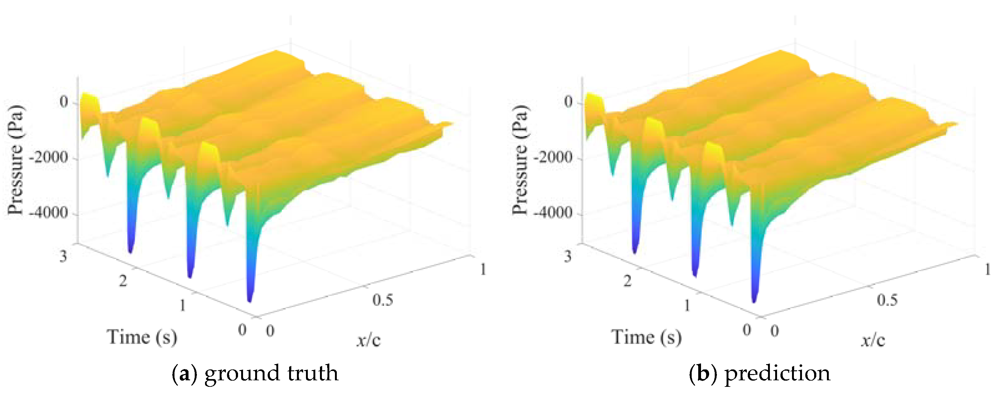
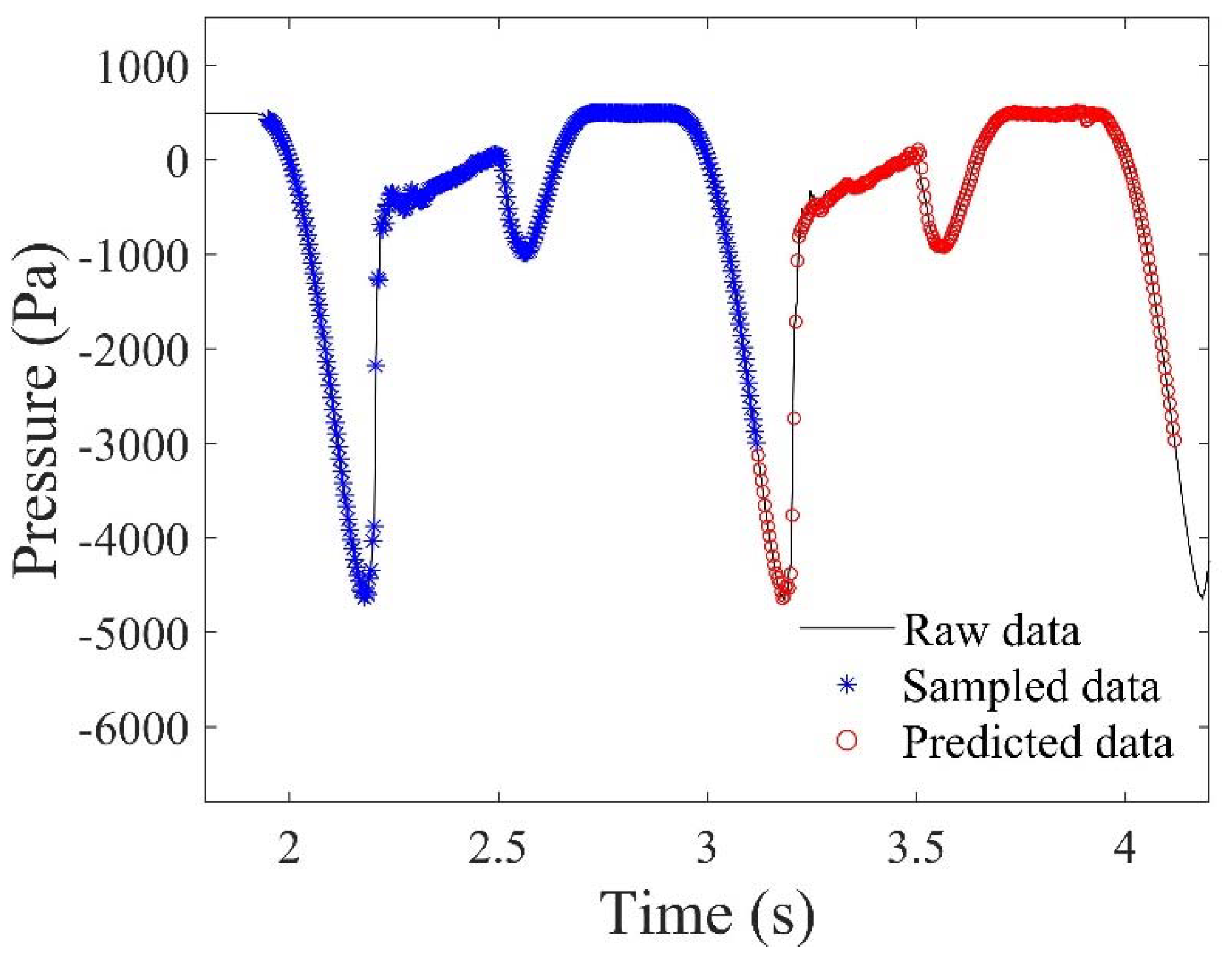
3.2. Prediction of Future Data

In this section, DMD with time delay embedding was used to reconstruct the history of pressure data of the oscillating airfoil. The high time-resolved pressure data collected by 20 sensors on the upper surface (see Table 1) were used in this method because the leading edge is the region with the most obvious pressure fluctuations. To examine the performance of this method, the error rate e between reconstructed data and true data is defined as:

$$e=\frac{1}{m}{\displaystyle \sum }_{t=1}^m\frac{\Vert P_{reconstructed,t}-P_{true,t}\Vert {}_2}{\Vert P_{true,t}\Vert {}_2}$$

(13)

where m is the number of used snapshots, $P_{reconstructed,t}$ is the reconstructed pressure field at time t, and $P_{true,t}$ is the true velocity field on the subdomain at time t.

POD analysis was applied to the time delay embedded dataset, and the mode energy spectrum is shown in Figure 6. The core of time delay embedding is the improvement of data dimensionality to capture more phase information. Therefore, the first three POD modes contained more than 98% energy. With the increase of the number of delay steps n_d, more POD modes were needed to reconstruct the data accurately. It should be noted that when the number of delay steps was increased to 200, the POD energy spectrum tended to be similar. In this experiment, one period contains 256 snapshots. Therefore, when n_d > 200, most of the phase information was included in the time delay embedded matrix.

The raw and reconstructed pressure data of sensor #1 were used to compare the reconstruction performance of the standard DMD and DMD with delay embedding. Sensor #1 is located at the leading edge, where the most obvious pressure fluctuations happen. The standard DMD (i.e., n_d = 0) and DMD with time-delay embedding were then applied to reconstruct the whole-time sequence of the pressure data. As shown in Figure 7a, standard DMD cannot accurately predict the dynamic pressure on sensor #1 even at the initial stage of the oscillation cycle. With time-delay embedding, the prediction performance is clearly improved. With n_d = 50 delay steps, DMD can capture the periodic trend, but with an underprediction of the oscillation amplitude and e ≈ 43%. With n_d increased to 200, the predicted values agree closely with the ground truth both in periodic trend and amplitude for more than six cycles and e ≈ 7%. Thus, DMD with time-delay embedding demonstrates the ability to reconstruct the periodic single-point pressure data over a long period. With an increasing number of delay steps n_d, the accuracy of the reconstruction is improved. However, an excessive number of delay steps will lead to too large a dimensionality of the matrix, which will not only consume computing and storage resources but negatively affect the real-time performance of the prediction algorithm. Therefore, the duration of the prediction cycle should be balanced with the requirement for computation time. In fact, the accurate prediction of just one cycle, that is, the next cycle, is usually helpful for effective decision-making in real-time control systems.

Based on the predicted pressures at single measurement points, DMD with time-delay embedding was then used to reconstruct the time-resolved pressure field on the upper surface of the airfoil. The ground truth of the pressure field obtained by 20 pressure sensors is shown in Figure 8a. The values reconstructed using DMD with time-delay embedding are shown in Figure 8b and match well with the measured data and accurately show the shape and peak of the three-dimensional surface.

The core of DMD is to find the Koopman operator, which allows the prediction of future data based on past data. The above section has demonstrated the accurate reconstruction of time-resolved pressure data using DMD with time-delay embedding, from which an optimal Koopman operator was obtained. Using the Koopman operator, real-time prediction can be realized. In Figure 9, the black line represents the ground-truth pressure data measured by sensor #1 over one oscillation period. The blue markers represent the past sampled pressure data that were used to build a new snapshot ${\mathrm{y}}_{\mathrm{j}}$. The future new snapshot $y_{j+1}$ was obtained based on the Koopman operator B provided by DMD with time-delay embedding, which had been verified in the above cases. Then, the future pressure data at the position of sensor #1 could be extracted from $y_{j+1}$. Furthermore, future snapshot $y_{j+2}$ can also be calculated with the help of a predicted snapshot $y_{j+1}$ in the same way. When this operation is repeated, the data for a long period of time in the future can be predicted. In Figure 9, 256 snapshots (a whole oscillation period) were predicted. The predicted next-step value accurately matches the ground-truth value, indicating the feasibility and potential of DMD with time delay embedding. The computation was implemented in MATLAB, and all the cases are run on an Intel Xeon E5-1620 at 3.50 GHz. Every prediction took 0.09 s. Admittedly, it is difficult to meet real-time requirements, but high-performance industrial computers can realize real-time prediction in practical applications. Work is ongoing to further improve the rapidity and adaptability of this method.

4. Conclusions

In this study, dynamic stall of oscillating airfoils was measured by dynamic pressure tapes and PSP visualization. The influence of the oscillation frequency was examined. Dynamic mode decomposition (DMD) with time-delay embedding was proposed to predict the pressure field on the oscillating airfoil based on scattered measurements. The major findings are as follows:

(1) Under the dynamic conditions of the oscillating airfoil, with increasing oscillation frequency, although lift coefficient can be improved at large AoAs, the aerodynamic characteristics showed a huge difference between upstroke and downstroke. The specific performance is that the loop hysteresis of both the lift and pitch moment coefficients were enlarged, which is detrimental to aerodynamic performance.

(2) DMD with time-delay embedding was able to reconstruct and predict dynamic stall based on scattered measurements with much higher accuracy than standard DMD. The reconstruction accuracy of this method increased with the number of delay steps, but this also prolonged the computation time. With the help of the Koopman operator obtained by DMD with time-delay embedding, the future dynamic pressure for a long time of an oscillating airfoil can be accurately predicted.

References

1. McCroskey, W.J. The Phenomenon of Dynamic Stall. NASA Tech. Memo. 1981, 81264, 1–28. [Google Scholar]
2. Mulleners, K.; Raffel, M. The onset of dynamic stall revisited. Exp. Fluids 2012, 52, 779–793. [Google Scholar] [CrossRef] [Green Version]
3. Chandrasekhara, M.S.; Carr, L.W.; Wilder, M.C. Interferometric investigations of compressible dynamic stall over a transiently pitching airfoil. AIAA J. 1994, 32, 586–593. [Google Scholar] [CrossRef] [Green Version]
4. Visbal, M.R. Dynamic stall of a constant-rate pitching airfoil. J. Aircraft 1990, 27, 400–407. [Google Scholar] [CrossRef]
5. Rival, D.; Tropea, C. Characteristics of pitching and plunging airfoils under dynamic-stall conditions. J. Aircraft 2010, 47, 80–86. [Google Scholar] [CrossRef] [Green Version]
6. Carr, L.W. Progress in analysis and prediction of dynamic stall. J. Aircraft 1988, 25, 6–17. [Google Scholar] [CrossRef]
7. Geissler, W.; Dietz, G.; Mai, H.; Bosbach, J.; Richard, H. Dynamic Stall and its passive control investigations on the OA209 airfoil section. In Proceedings of the 31st European Rotorcraft Forum 2005 (ERF31), Florence, Italy, 13–15 September 2005. [Google Scholar]
8. Heine, B.; Mulleners, K.; Joubert, G.; Raffel, M. Dynamic stall control by passive disturbance generators. AIAA J. 2013, 51, 2086–2097. [Google Scholar] [CrossRef] [Green Version]
9. Konstantinidis, E.; Balabani, S. Symmetric vortex shedding in the near wake of a circular cylinder due to streamwise perturbations. J. Fluids Struct. 2007, 23, 1047–1063. [Google Scholar] [CrossRef]
10. Melton, L.P.; Koklu, M.; Andino, M.; Lin, J.C. Active flow control via discrete sweeping and steady jets on a simple-hinged flap. AIAA J. 2018, 56, 2961–2973. [Google Scholar] [CrossRef]
11. Schmidt, H.J.; Woszidlo, R.; Nayeri, C.N.; Paschereit, C.O. Separation control with fluidic oscillators in water. Exp. Fluids 2017, 58, 1–17. [Google Scholar] [CrossRef]
12. Gao, D.; Chen, G.; Chen, W.; Huang, Y.; Li, H. Active control of circular cylinder flow with windward suction and leeward blowing. Exp. Fluids 2019, 60, 26. [Google Scholar] [CrossRef]
13. Patel, M.P.; Carver, R.; Lisy, F.J.; Prince, T.S.; Ng, T. Detection and control of flow separation using pressure sensors and micro-vortex generators. In Proceedings of the 40th AIAA Aerospace Sciences Meeting & Exhibit, Reno, NV, USA, 14–17 January 2002. [Google Scholar] [CrossRef]
14. Saini, A.; Gopalarathnam, A. Leading-edge flow sensing for aerodynamic parameter estimation. AIAA J. 2018, 56, 4706–4718. [Google Scholar] [CrossRef]
15. Le Provost, M.; He, X.; Williams, D.R. Real-time roll moment identification with distributed surface pressure sensors on a rolling UCAS wing. In Proceedings of the AIAA Aerospace Sciences Meeting, Kissimmee, FL, USA, 8–12 January 2018. [Google Scholar]
16. Juliano, T.J.; Peng, D.; Jensen, C.; Gregory, J.W.; Liu, T.; Montefort, J.; Palluconi, S.; Crafton, J.; Fonov, S. PSP measurements on an oscillating NACA 0012 airfoil in compressible flow. In Proceedings of the 41st AIAA Fluid Dynamics Conference and Exhibit, Honolulu, HI, USA, 27–30 June 2011. [Google Scholar] [CrossRef]
17. An, X.; Williams, D.R.; Eldredge, J.D.; Colonius, T. Lift coefficient estimation for a rapidly pitching airfoil. Exp. Fluids 2021, 62, 1–12. [Google Scholar] [CrossRef]
18. Gao, Y.; Zhu, Q.; Wang, L. Measurement of unsteady transition on a pitching airfoil using dynamic pressure sensors. J. Mech. Sci. Technol. 2016, 30, 4571–4578. [Google Scholar] [CrossRef]
19. Sabater, C.; Stürmer, P.; Bekemeyer, P. Fast Predictions of Aircraft Aerodynamics using Deep Learning Techniques. In Proceedings of the AIAA AVIATION 2021 FORUM, Online, 2–6 August 2021. [Google Scholar] [CrossRef]
20. Singh, A.P.; Medida, S.; Duraisamy, K. Machine-learning-augmented predictive modeling of turbulent separated flows over airfoils. AIAA J. 2017, 55, 2215–2227. [Google Scholar] [CrossRef]
21. Meyer, K.E.; Pedersen, J.M.; Özcan, O. A turbulent jet in crossflow analysed with proper orthogonal decomposition. J. Fluid Mech. 2007, 583, 199–227. [Google Scholar] [CrossRef] [Green Version]
22. Dawson, S.T.M.; Schiavone, N.K.; Rowley, C.W.; Williams, D.R. A data-driven modeling framework for predicting forces and pressures on a rapidly pitching airfoil. In Proceedings of the 45th AIAA Fluid Dynamics Conference, Dallas, TX, USA, 22–26 June 2015. [Google Scholar] [CrossRef] [Green Version]
23. Bright, I.; Lin, G.; Kutz, J.N. Compressive sensing based machine learning strategy for characterizing the flow around a cylinder with limited pressure measurements. Phys. Fluids 2013, 25, 127102. [Google Scholar] [CrossRef]
24. Zhou, K.; Zhou, L.; Zhao, S.; Qiang, X.; Liu, Y.; Wen, X. Data-Driven Method for Flow Sensing of Aerodynamic Parameters Using Distributed Pressure Measurements. AIAA J. 2021, 59, 3504–3516. [Google Scholar] [CrossRef]
25. Saini, A.; Narsipur, S.; Gopalarathnam, A. Leading-edge flow sensing for detection of vortex shedding from airfoils in unsteady flows. Phys. Fluids 2021, 33, 21–28. [Google Scholar] [CrossRef]
26. Pinier, J.T.; Ausseur, J.M.; Glauser, M.N.; Higuchi, H. Proportional closed-loop feedback control of flow separation. AIAA J. 2007, 45, 181–190. [Google Scholar] [CrossRef]
27. Zhao, X.; Kania, R.; Kebbie-Anthony, A.; Azarm, S.; Balachandran, B. Dynamic data-driven aeroelastic response prediction with discrete sensor observations. In Proceedings of the 2018 AIAA Non-Deterministic Approaches Conference, Kissimmee, FL, USA, 8–12 January 2018; pp. 1–12. [Google Scholar] [CrossRef]
28. Schmid, P.J. Dynamic mode decomposition of numerical and experimental data. J. Fluid Mech. 2010, 656, 5–28. [Google Scholar] [CrossRef] [Green Version]
29. Berger, E.; Sastuba, M.; Vogt, D.; Jung, B.; Ben Amor, H. Dynamic Mode Decomposition for perturbation estimation in human robot interaction. In Proceedings of the The 23rd IEEE International Symposium on Robot and Human Interactive Communication, Edinburgh, UK, 25–29 August 2014; pp. 593–600. [Google Scholar] [CrossRef]
30. Le Clainche, S.; Vega, J.M. Higher order dynamic mode decomposition. SIAM J. Appl. Dyn. Syst. 2017, 16, 882–925. [Google Scholar] [CrossRef] [Green Version]
31. Brunton, S.L.; Brunton, B.W.; Proctor, J.L.; Kaiser, E.; Nathan Kutz, J. Chaos as an intermittently forced linear system. Nat. Commun. 2017, 8, 1–8. [Google Scholar] [CrossRef]
32. Murshed, M.N.; Monir Uddin, M. Time delay coordinate based dynamic mode decomposition of a compressible signal. In Proceedings of the 2019 22nd International Conference on Computer and Information Technology, ICCIT, Dhaka, Bangladesh, 18–20 December 2019; pp. 18–20. [Google Scholar]
33. Susuki, Y.; Sako, K. Data-Based Voltage Analysis of Power Systems via Delay Embedding and Extended Dynamic Mode Decomposition. IFAC-PapersOnLine 2018, 51, 221–226. [Google Scholar] [CrossRef]
34. Pan, S.; Duraisamy, K. On the structure of time-delay embedding in linear models of non-linear dynamical systems. Chaos 2020, 30, 073135. [Google Scholar] [CrossRef]
35. Yuan, Y.; Zhou, K.; Zhou, W.; Wen, X.; Liu, Y. Flow prediction using dynamic mode decomposition with time-delay embedding based on local measurement. Phys. Fluids 2021, 33, 095109. [Google Scholar] [CrossRef]
36. Arbabi, H.; Korda, M.; Mezić, I. A data-driven Koopman model predictive control framework for nonlinear ows. In Proceedings of the The 57th IEEE Conference on Decision and Control, Miami Beach, FL, USA, 17–19 December 2018; pp. 6409–6414. [Google Scholar]
37. Miller, S.D. Lift, Drag and Moment of a NACA 0015 Airfoil. Available online: https://smiller.sbyers.com/temp/AE510_03%20NACA%200015%20Airfoil.pdf (accessed on 6 December 2021).
38. Williams, M.O.; Kevrekidis, I.G.; Rowley, C.W. A Data–Driven Approximation of the Koopman Operator: Extending Dynamic Mode Decomposition. J. Nonlinear Sci. 2015, 25, 1307–1346. [Google Scholar] [CrossRef] [Green Version]
39. Dellnitz, M.; Von Molo, M.H.; Ziessler, A. A kernel-based method for data-driven Koopman spectral analysis. J. Comput. Dyn. 2016, 2, 247–265. [Google Scholar] [CrossRef]
40. Mai, H.; Dietz, G.; Geißler, W.; Richter, K.; Bosbach, J.; Richard, H.; Groo, K. De Dynamic stall control by leading edge vortex generators. Annu. Forum Proc. AHS Int. 2006, III, 1728–1739. [Google Scholar]
Figure 1. Schematic of a measurement system using pressure and PSP.
Actuators 11 00046 g001
Figure 2. PSP visualization of the dynamic pressure on the oscillating airfoil with f = 1 Hz. (The horizontal direction is the full chord length, and the vertical direction is the spanwise direction).
Actuators 11 00046 g002
Figure 3. Static stall characteristics are shown in coefficients of (a) lift (Cl) and (b) pitch moment (Cm) for the static airfoil.
Actuators 11 00046 g003
Figure 4. Phase-averaged lift coefficient (Cl) at frequencies of (a) f = 1 Hz, (b) f = 2 Hz, (c) f = 3 Hz, and (d) f = 4 Hz for oscillating airfoils.
Actuators 11 00046 g004
Figure 5. Phase-averaged moment coefficient (Cm) for (a) f = 1 Hz, (b) f = 2 Hz, (c) f = 3 Hz, and (d) f = 4 Hz for the oscillating airfoil.
Actuators 11 00046 g005
Figure 6. POD mode energy spectrum of the time-delay embedded data with different nd.
Actuators 11 00046 g006
Figure 7. Reconstruction of pressure data measured by sensor #1 (see Table 1) using (a) standard DMD and time-delay embedding DMD with number of delay steps (b) nd = 50, (c) nd = 100, and (d) nd = 200.
Actuators 11 00046 g007
Figure 8. Pressure field on the upper surface of the oscillating airfoil: (a) ground-truth data from pressure sensors, (b) reconstruction using DMD with time-delay embedding.
Actuators 11 00046 g008
Figure 9. Prediction of future pressure data based on Koopman operator obtained by DMD with time-delay embedding.
Actuators 11 00046 g009