1. Introduction
In a wide range of robotic applications, for example, assembly of electronic boards or handling of objects to be placed on horizontal pallets, the full mobility (6-DOF) of the end-effector is not necessary, since the tasks can be proficiently performed by means of a 3-DOF translational motion or by a 4-DOF motion with three translations and one rotation around a vertical axis (Schoenflies motion [
1]). The rotational degree of freedom of the Schoenflies motion is often obtained by adding a 1-DOF wrist to a translational mechanism.
Considering serial robots, translational and Schoenflies motions are realized in most cases by Cartesian robots or by SCARA robots [
2,
3,
4,
5]. Considering parallel kinematics machines (PKMs), translational motion can be obtained by parallel Cartesian robots [
6,
7,
8], characterized by three legs that are planar serial mechanisms moved by three orthogonal linear actuators perpendicularly to their planes, or by other closed-loop schemes which are not purely translational in general, but become purely translational in case of specific orientations of the joint axes [
1,
9,
10,
11]. If necessary, translational PKMs can be upgraded to Schoenflies motions by a 1-DOF wrist, but there are also some designs of PKMs which perform native Schoenflies motions [
12,
13].
No matter if it is serial or parallel, a robot can be controlled in position if the task can be correctly performed regulating only the end-effector trajectory, or by hybrid position/force control when the proper execution of the task requires accurate force regulation in some phases and in some directions [
14]. An intermediate approach, which is widely adopted since it does not require force sensors, is represented by impedance control [
15,
16].
The basic concept of impedance control is that the robot end-effector, subject to external forces, follows a trajectory with a predetermined spatial compliance. The relationship between the force/moment exerted by the end-effector on the environment and the end-effector position/orientation error is defined by means of the stiffness and damping matrices. This approach allows to obtain a compliant behavior in the directions which must be force-controlled, and a stiff behavior in the directions which must be position-controlled.
There are many possible ways to the define the orientation of a rigid body in space [
17], and this results in different possible approaches for the definition of the rotational stiffness/damping in impedance control [
18,
19,
20,
21]. On the contrary, for translational robots, the approach to impedance control is much less diversified and simpler, since a point position in space is always represented using an orthogonal reference frame. Additionally, in case of a robot with Schoenflies motion, impedance control is simplified, since the rotation is mono-dimensional, and the rotational behavior is decoupled from the translational behavior. In this work, we will consider only translational impedance control, considering that it can be easily extended to robots with Schoenflies motion.
For translational robots, the impedance behavior of the end-effector is usually defined by means of the stiffness and damping matrices, which respectively represent the zero-order and the first-order terms of a three-dimensional PD control in the external coordinates, expressed in the principal reference frame. These matrices are non-diagonal in the world frame when the principal stiffness and damping directions are not parallel to the axes of the fixed reference frame [
11].
Some authors have proposed nonlinear impedance algorithms, in which nonlinear stiffness and damping are imposed to the end-effector, in particular for a better execution of cooperative human–robot tasks, or to maintain position/orientation within a specified region even in case of excessive forces/moments [
22,
23,
24].
An alternative method to define the impedance behavior is based on fractional calculus, which introduces derivatives and integrals of non-integer order [
25]. Accordingly, the damping term can be defined proportional not to the first-order derivative of the end-effector error, but to a derivative with generic non-integer order
μ. In the scientific literature, there are some examples of fractional-order impedance controls of robots [
26,
27]. This kind of impedance control generalizes to a three-dimensional system the fractional-order PD
μ control scheme for SISO systems [
28]. Fractional-order impedance can be used, for example, to perform contact force tracking control more accurately than traditional impedance control [
29].
In the proposed work, the stiffness/damping behavior imposed by the impedance control is linear, but a half-order term, based on the fractional derivative of order 1/2 of the position error, is added to the zero-order and first-order terms of classical impedance control. This impedance control generalizes to a three-dimensional system the fractional-order PDD
1/2 control scheme developed, so far, for single axes [
30].
As a matter of fact, it is evident that traditional linear impedance control of a
n-DOF mechanical system (KD) is the
n-dimensional version of the PD control of a 1-DOF mechanical system, with the
n-dimensional stiffness term K, proportional to the position error, corresponding to the proportional term, and the
n-dimensional damping term D, proportional to the first-order derivative of the position error, corresponding to the derivative term. The proposed KDHD impedance control is obtained from the KD scheme with the addition of an
n-dimensional half-order damping term HD, proportional to the derivative of order 1/2 (half-derivative) of the position error; therefore, the aim of this work is to investigate if the addition of the half-derivative term in the implementation of the impedance algorithm can bring the same benefits that have been shown theoretically and experimentally for the PDD
1/2 control of a 1-DOF inertial system with respect to the classical PD scheme [
31].
As a case study, the KDHD impedance control is applied to a 3-PUU parallel robot and compared to the classical KD impedance control.
In the remainder of the paper,
Section 2 discusses the theoretical definition and the digital implementation of the half-derivative of a function of time,
Section 3 proposes the KDHD impedance control, highlighting the differences with respect to the classical KD impedance control, and
Section 4 presents the 3-PUU architecture and its kinematics.
Section 5 compares the KDHD and the KD impedance controls applied to the 3-PUU robot by multibody simulation, and
Section 6 outlines conclusions and future developments.
2. Half-Order Derivative: Definition and Digital Implementation Issues
Fractional calculus generalizes the concept of derivative and integral to non-integer order [
25]. According to the Grünwald–Letnikov definition, suitable for robust discrete-time implementation [
32], the fractional differential operator for a continuous function of time,
x(t), is defined as:
where
is the differentiation order,
a and
t are the fixed and variable limits, Γ is the Gamma function,
h is the time increment, and [
y] is the integer part of
y. For real-time digital implementation with sampling time
Ts, Equation (1) can be rewritten in the following form [
31]:
where:
The calculation of Equation (2) requires considering all the
k + 1 sampled values of the time history of
x; therefore, the incessant increase of the number of addends is an issue for real-time implementation, and consequently, only a fixed number of
n previous steps is used in Equation (2), realizing a
nth order digital filter, with fixed memory length
L = nTs. This is acceptable according to the so-called short-memory principle [
33], which states that considering only the recent past of the function in the interval [
t–L, t] does not yield relevant approximations in the evaluation of the fractional derivative.
Nevertheless, the truncation of the summation of Equation (2) to
n + 1 addends is an issue if the fractional derivative is applied to impedance control. As a matter of fact:
but with finite
n, this summation is non-null:
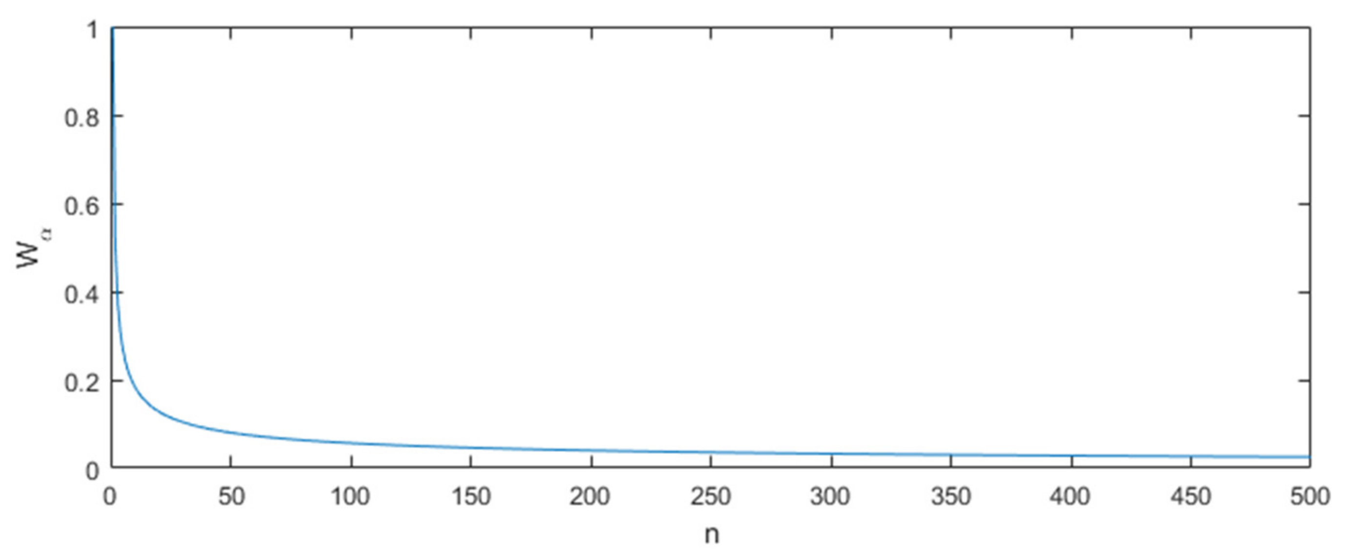
Moreover,
Wα tends to zero quite slowly, as shown in
Figure 1, as an example, for
α = 1/2 (half-derivative).
As a consequence, the numerically evaluated fractional derivative of a constant c is non-null, but equal to , tending to zero as n tends to infinite. This influences the behavior of impedance control in the steady state, giving rise to a constant position error. In this condition, only the stiffness term should be non-null, but if fractional-order damping is numerically evaluated with a finite-order digital filter, the half-derivative damping term is also present, and should be properly compensated.
3. KDHD Impedance Control
The classical formulation of impedance control with gravity compensation of a non-redundant parallel robot is expressed by the following control law [
11]:
where
Jp is the Jacobian matrix for a parallel robot, which defines the relationship between the time-derivative of the external coordinates
x and the time-derivative of the internal coordinates
q:
In Equation (6), KKD and DKD are the stiffness and damping matrices, xd is the reference trajectory expressed in external coordinates, and τg is the gravity compensation vector.
Let us note that the matrices
KKD and
DKD, on the basis of the robot mobility, define the translational impedance, the rotational impedance, or both [
21]. In case of robots with Schoenflies motion, their size is 4 × 4, but the rotational behavior is evidently decoupled from the translational behavior; therefore, the stiffness and damping matrices are block-diagonal, with a 3 × 3 submatrix representing the translational behavior and a fourth diagonal element representing the rotational behavior. In the following, for the sake of simplicity, we will consider translational robots with 3 × 3 stiffness and damping matrices, bearing in mind that the proposed approach can be easily extended to robots with Schoenflies motion.
The stiffness and damping matrices are in general non-diagonal in the fixed reference frame, W. On the basis of the task requirements, it is possible to choose a principal reference frame, P, in which it is convenient to define decoupled stiffness and damping; therefore, the stiffness and damping matrices are defined diagonal in P and are transformed into the frame W by means of the rotation matrix between W and P [
21]:
In the proposed KDHD impedance control, the damping term is not proportional only to the first-order derivative of the position error in external coordinates, but also to its half-derivative (derivative of order 1/2), in order to implement the extension from PD to PDD
1/2 in the three-dimensional space:
Obviously, the half-derivative damping matrix
HDKDHD can also be defined in the principal reference frame, P, and then transformed to the frame W:
Let us note that in the definition of the KDHD impedance control law, a non-redundant parallel robot has been considered. In case of non-redundant serial robots, the approach is similar, but it is more convenient to adopt the Jacobian matrix, which transfers from internal coordinates’ derivatives to external coordinates’ derivatives [
2]:
Consequently, for application to non-redundant serial robots, the impedance control laws (6) and (10) can be rewritten in the following form:
4. Kinematic and Dynamic Model of the 3-PUU Parallel Robot
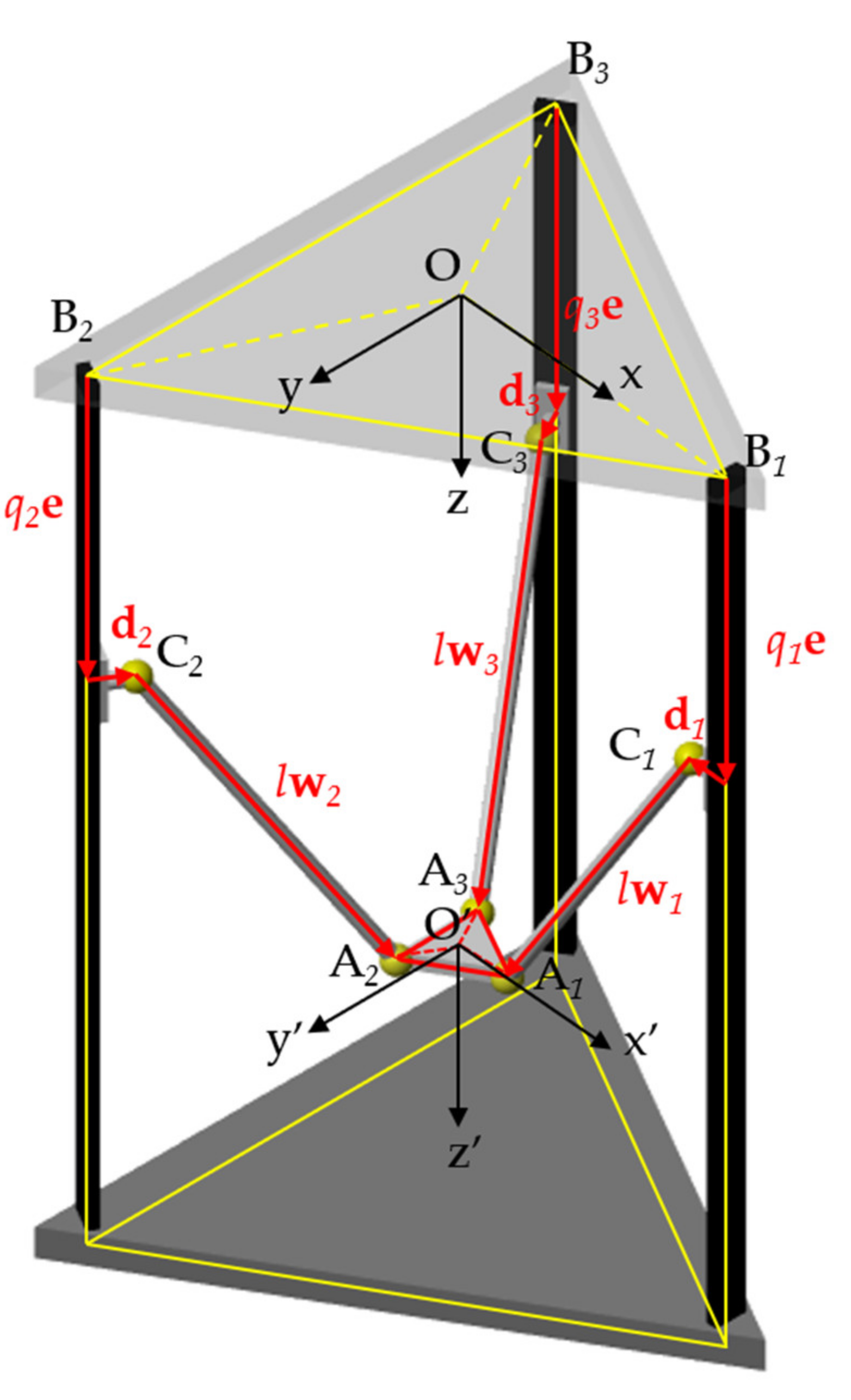
The proposed KDHD impedance control has been tested by multibody simulation on the 3-PUU parallel robot, whose scheme is shown in
Figure 2.
The reference frame O(x,y,z) of the base platform is located at the center of the equilateral triangle B
1B
2B
3, whose vertices lie on a circumference with center O and radius
R, while the reference frame O’(x’,y’,z’) of the moving platform is located at the center of the equilateral triangle A
1A
2A
3, whose vertices lie on a circumference with center O’ and radius
r. The unit vector
e, perpendicular to the plane of the triangle B
1B
2B
3, defines the direction of the three prismatic joints, and the vector of the internal coordinates
q = [
q1, q2, q3]
T is composed by the distances of the centers of the three sliders from the points B
1, B
2, and B
3; consequently, the three vectors,
q1e,
q2e, and
q3e, represent the displacements of the sliders’ centers with respect to B
1, B
2, and B
3. For constructive reasons, the centers of the universal joints mounted on the sliders do not lie on the prismatic joints’ axes, but are shifted by the three vectors
di,
i = 1…3, with equal module
d and the direction of the vector (O–B
i). Six universal joints are located at the points C
1, C
2, C
3, A
1, A
2, and A
3. In order to obtain purely translational motion of the moving platform, in each PUU kinematic chain, the first revolute axis of the upper U joint must be parallel to the first revolute axis of the lower U joint, and the second revolute axis of the upper U joint must be parallel to the second revolute axis of the lower U joint [
34].
5. Comparison of the KD and KDHD Impedance Control Laws by Multibody Simulation
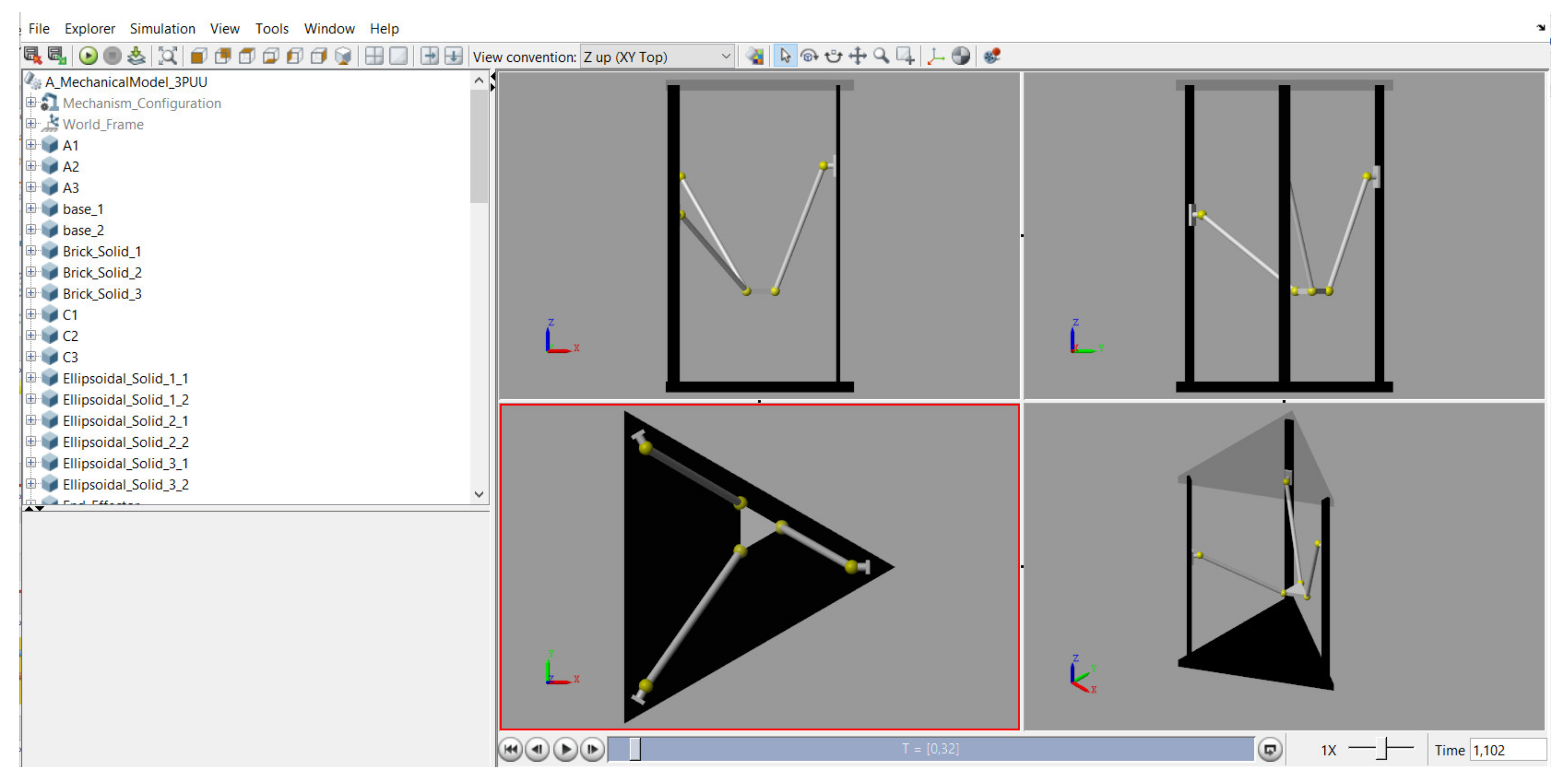
5.1. Modeling and Simulation Overview
The model of the 3-PUU parallel robot has been implemented in the multibody simulation environment Simscape Multibody
TM by MathWorks (
Figure 3). The robot geometrical and inertial parameters considered in the simulations are collected in
Table 1.
The proposed KDHD impedance control law has been compared to KD impedance control in the following case studies.
(A) End-effector reference trajectory, xd, characterized by displacements along the three directions with trapezoidal speed laws, no external force on the end-effector, and the end-effector behavior is isotropic: the stiffness and damping matrices are diagonal with three equal elements. This case represents an approach/depart motion without contact with the environment.
(B) Constant end-effector reference position and external force applied to the end-effector. The stiffness and damping matrices are diagonal in the world frame (the fixed reference frame, W, coincides with the principal stiffness/damping reference frame, P), but the end-effector behavior is not isotropic, since the three diagonal elements are not equal. This case study evidences how with the KDHD scheme, the approximation of the half-derivative calculation by means of a digital filter with a fixed memory length alters the stiffness imposed by impedance control, as discussed in
Section 2; consequently, the stiffness matrix must be properly compensated. A compensation method (KDHDc) is proposed, and its effectiveness is validated by simulation.
(C) Constant end-effector reference position and external force applied to the end-effector, as in case B, but with non-diagonal stiffness and damping matrices, since the fixed reference frame, W, does not coincide with the principal stiffness/damping reference frame, P. Additionally, in this case, the effectiveness of the proposed stiffness-compensated KDHDc impedance control is validated by simulation.
In all the case studies, gravity force is neglected, since its effect is exactly compensated by the gravity compensation term, which is equal for all the considered impedance controls schemes. This allows to better highlight the differences between the KD, KDHD, and KDHDc schemes, eliminating the equal contribution to the actuation forces due to gravity.
Impedance control is based on the measurement of the internal coordinates of the robot without measurement of the force exerted by the end-effector on the environment, as in the case of hybrid position/force control. The internal coordinates of the robot, both for rotational and for linear actuators, are measured by digital encoders, which are not affected by noise; therefore, we have decided not to take into account noise on the measured position of the three sliders.
On the other hand, some noise is certainly present on the actuation forces, due to the electrical effects of the current loop of the motor drivers; nevertheless, the sensitivity of the closed-loop transfer function to disturbances on the direct path, which comprises the motor driver, is much lower than the sensitivity to disturbances on the feedback path. Consequently, noise has been neglected in the first stage of the research.
5.2. Case Study A
In this case study, the stiffness and damping matrices are diagonal and isotropic both for the KD and KDHD impedance controls. For the KD scheme:
where
I is the identity matrix. The diagonal value,
dKD, of the damping matrix can be selected starting from the nondimensional damping coefficient,
ζKD, according to the following expression [
35]:
in which the mass,
mmp, of the moving platform (including the three lower universal joints) is considered.
For the KDHD scheme, the stiffness matrix and the first-order and half-order damping matrices are:
The diagonal values
dKDHD and
hdKDHD of the damping matrices can be selected starting from the nondimensional coefficients
ζKDHD and
ψKDHD, according to the following expressions:
The coefficients
ζKDHD and
ψKDHD non-dimensionally represent the derivative and half-derivative damping terms [
35]. In [
36], three couples of PD and PDD
1/2 tunings are compared in the control of a linear axis (
Table 2).
These three couples of PD and PDD
1/2 tunings have been selected as starting points of the research using the nondimensional approach discussed in [
36] to derive the coefficients
ζ and
ψ of a PDD
1/2 controller from the coefficient
ζ of a reference PD controller, with application to a nondimensional second-order purely inertial linear system, with transfer function
G(s) = 1/s2. This method can be summarized as follows:
- -
A PD closed-loop control with a given ζ is applied to the position control of G(s), considering a step input.
- -
The settling energy of the step response is calculated.
- -
There are infinite combinations of ζ and ψ for a PDD1/2 controller with the same proportional gain which are characterized by the same settling energy of the PD. The ζ–ψ combination which minimizes the settling time is selected.
Table 2 collects the PDD
1/2 ζ–
ψ combinations associated to three reference PD controllers, with
ζ = 0.8, 1, and 1.2. The basic idea of this approach is to obtain a PDD
1/2 tuning with a similar control effort as the corresponding PD tuning, but with improved readiness. Since this approach is nondimensional, the association between the coefficient
ζ of the PD and the
ζ–
ψ combination of the PDD
1/2 controller is not influenced by the system mass/inertia nor by the proportional gain; moreover, even if this approach is based on the step input, the benefits in terms of control readiness of the PDD
1/2 controller are also demonstrated with different reference inputs [
36].
The stiffness and damping matrices for the KD and KDHD impedance controls have been obtained starting from the nondimensional values of
Table 2, imposing
kKD =
kKDHD = 1·10
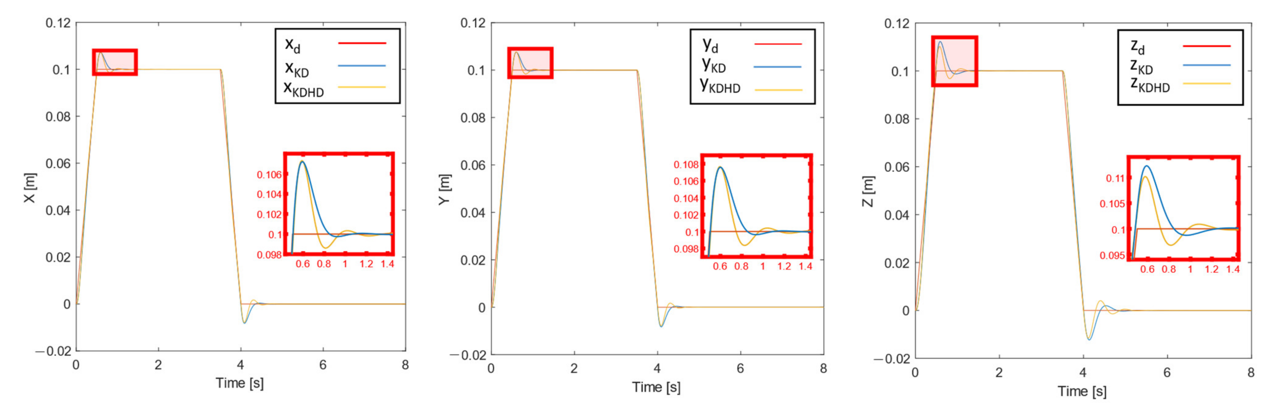
3 N/m and using Equations (15) to (22); then, the two control laws have been compared in the presence of a trapezoidal reference trajectory,
xd, characterized by four phases:
Constant velocity from (0, 0, zd,in) to (0.1, 0.1, 0.1 + zd,in) [m], where zd,in is the initial z-coordinate of the end-effector, which does not influence the simulation results due to the architecture of the PKM, with three sliders aligned along the fixed frame z-axis. The duration of this phase is tramp.
xd remains constant in (0.1, 0.1, 0.1 + zd,in) [m] for tstop.
xd returns to (0, 0, zd,in) [m] with constant velocity in tramp.
xd remains constant in (0, 0, zd,in) [m] for tstop.
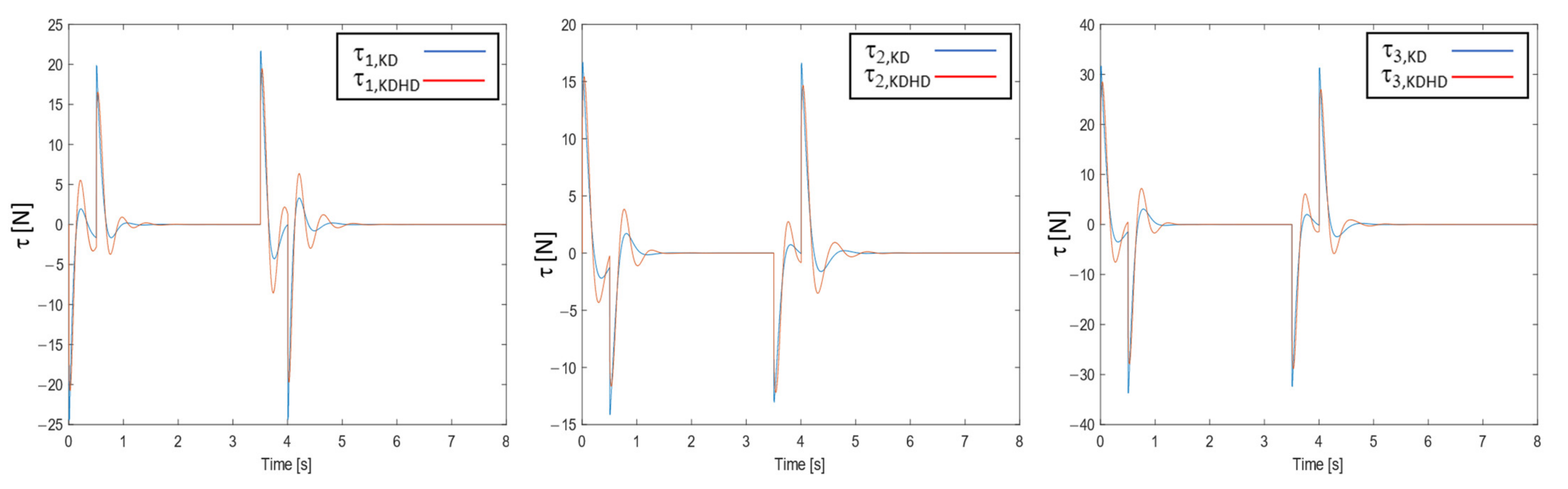
Some simulation results are shown in
Figure 4 and
Figure 5, with reference to the KD-KDHD comparison number I (
ζKD = 0.8,
Table 2), ramp time
tramp = 0.5 s, and stop time = 3 s.
Table 3 summarizes the results of the case study A with the three considered KD-KDHD tuning couples of
Table 2, and with two different ramp times (0.5 and 1 s), while the stop time has been kept constant at 3 s, sufficient to reach the settling time to within 2% after phases 1 and 3. The half-derivative is calculated using Equation (2) with sampling time
Ts = 0.005 s and filter order
n = 10, and these values are suitable for a real-time digital implementation on a commercial controller. The total control effort related to the three motors, reported in
Table 3, is defined as:
where
Tsim is the simulation time.
Comparing the performances of the two impedance controllers in the six cases of
Table 3, it is possible to observe the following outcomes:
- -
The KDHD control has lower integral absolute errors of all the external coordinates in all the cases (average variation with respect to KD: −25.0%), and has lower maximum actuation forces for all three motors in all the cases (average variation with respect to KD: −17.6%). This is the most interesting aspect, because it means that the KDHD control can reduce the tracking error with same size of actuators; moreover, this confirms that the extension from KD to KDHD has benefits similar to the extension from PD to PDD
1/2 [
31], supposed as the starting point of the investigation.
- -
Considering the maximum error, in most cases, the KDHD is better than the KD, but not for all the external coordinates and for all the cases, such as for the integral absolute error; however, the average reduction of the maximum error is −3.4%.
- -
The settling time to within 2% of the commanded displacement is in general better for the KDHD, with an average reduction over the six cases and over the three external coordinates of −25.8%.
- -
The total control effort is higher for the KDHD with respect to KD, with an average increase over the six cases and over the three external coordinates of +24.7%.
In [
31], a detailed discussion of the PDD
1/2 tuning of a second-order, purely inertial system is outlined, and these tuning criteria can be applied to the KDHD impedance control tuning, bearing in mind that the nonlinearity of a MIMO system as an impedance-controlled PKM introduces some alterations in the three-dimensional extension of the PDD
1/2 concept.
Let us note that the considered trapezoidal reference position law is characterized by velocity steps and impulsive accelerations in 0,
tramp, (
tramp +
tstop), and (2
tramp +
tstop); consequently, the position error cannot be completely eliminated, not even adopting a model-based control scheme, since infinite actuation forces would be required. Accordingly, some overshoot is unavoidable in the transitory states after the discontinuities in
tramp and (2
tramp +
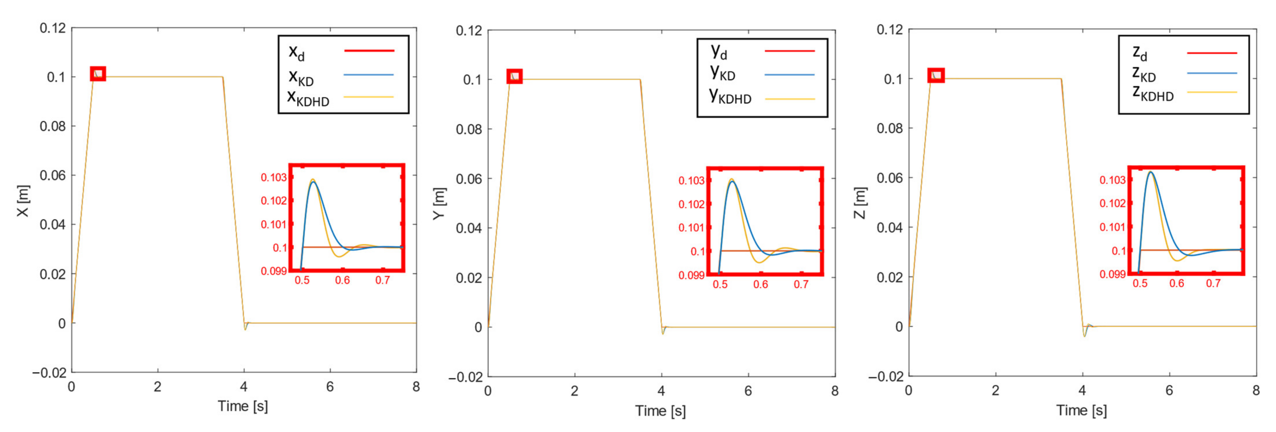
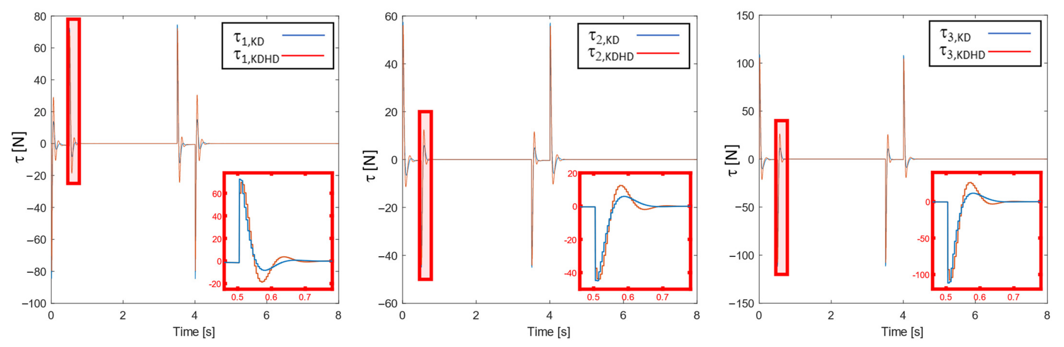
tstop). A smoother reference law for position, for example, with cycloidal or trapezoidal speed, would decrease the position error; nevertheless, here, a trapezoidal position law was adopted to highlight the differences between the KD and the KDHD impedance controls in trajectory tracking. The position error can be reduced by using higher stiffness, with increasing force peaks; for example,
Figure 6 and
Figure 7 represent the external coordinates and the actuation forces for the same KD-KDHD comparison of
Figure 4 and
Figure 5 (comparison number I, ramp time
tramp = 0.5 s, stop time
tstop = 3 s), but with
kKD =
kKDHD = 1·10
4 N/m. The maximum error of the external coordinates is lower, but the actuation forces are higher.
5.3. Case Study B
In this case study, the stiffness and damping matrices are diagonal in the world frame, but the desired end-effector behavior is not isotropic; therefore, the three diagonal elements of each matrix are not equal as in case study A. We impose higher compliance on the
z-axis through the following values:
kKD,x =
kKDHD,x =
kKD,y =
kKDHD,y = 2·10
4 N/m,
kKD,z =
kKDHD,z = 1·10
3 N/m. The diagonal values of the damping matrices are obtained as in case A, starting from the nondimensional parameters of
Table 2 and using Equations (17), (21), and (22) separately for each axis. A force
F = [100,100,100]
T N is applied to the end-effector at
t = 0 s. The half-derivative is calculated adopting the same discrete-time implementation as in case A (
Ts = 0.005 s,
n = 10).
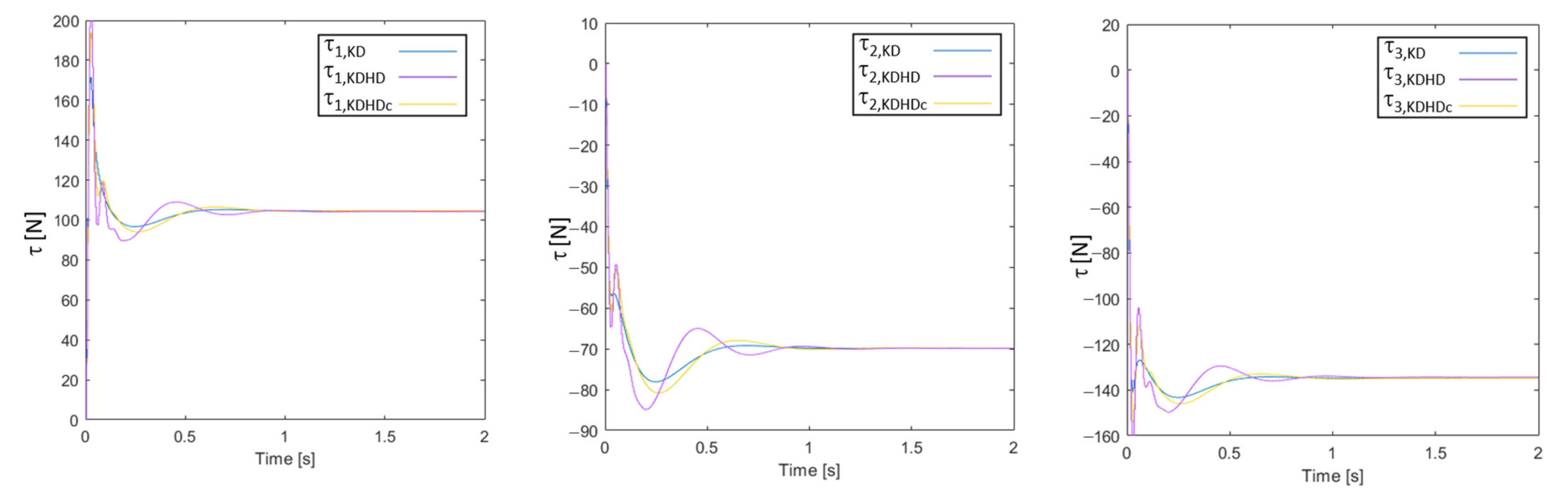
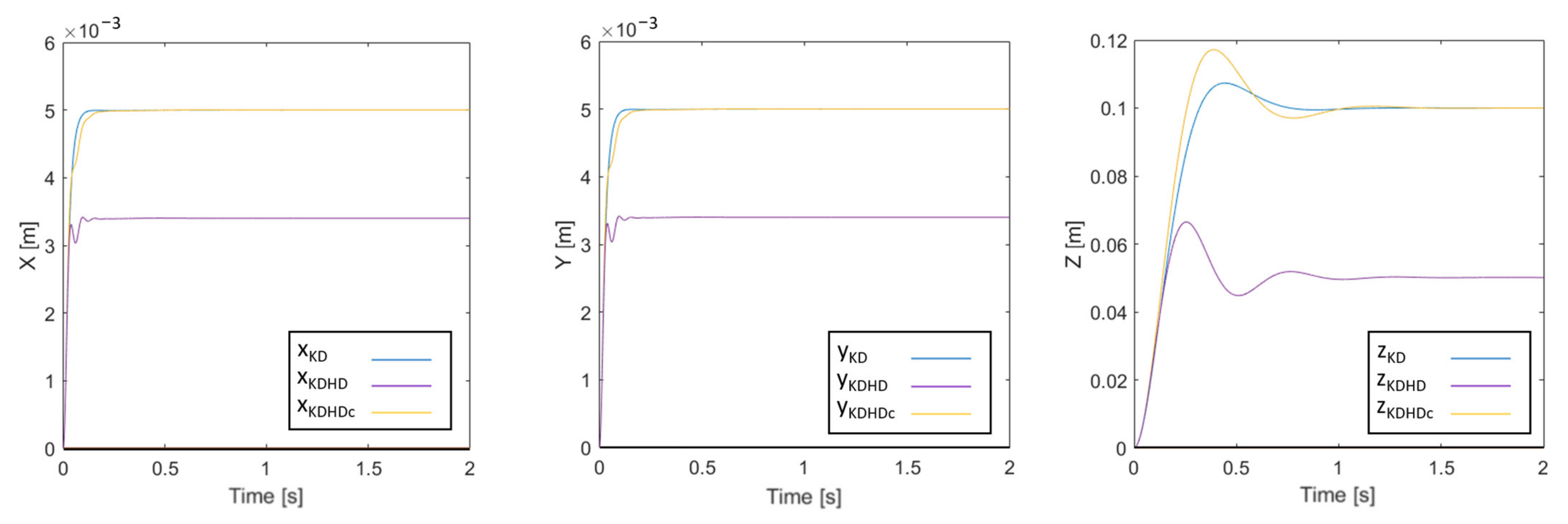
Figure 8 and
Figure 9 show the simulation results with reference to the KD-KDHD comparison number II (
ζKD = 1,
Table 2), in terms of external coordinates and actuation forces. Observing
Figure 8, it is possible to note that the steady-state displacements of the external coordinates using the impedance control KD (blue) and KDHD (violet) are different. This is due to the fact, already discussed in
Section 2, that the approximation of the half-derivative calculation by means of a digital filter with a fixed memory length alters the stiffness imposed by impedance control. As a matter of fact, considering that the half-derivative of a constant
c is non-null, but equal to
cW1/2(n)/(Ts)1/2, as discussed at the end of
Section 2, the following stiffness-compensated KDHD impedance control (KDHDc) is proposed:
The effectiveness of this stiffness compensation is validated by the fact that applying the KDHDc control law, the external coordinates (
Figure 8, yellow) tend to the same values obtained by applying the KD control law, which is not affected by the stiffness alteration due to the numerical evaluation of the half-derivative; as expected, these steady-state values correspond to the force/stiffness ratios
Fx/kKD,x,
Fy/kKD,y, and
Fz/kKD,z for the three directions. Let us note that, due to the definition of
Wα, this compensation is correct only in the steady state with a constant position reference, which are the conditions for which it has been introduced to obtain a correspondence between steady-state force and displacement.
5.4. Case Study C
In this case study, the stiffness compensation of the impedance control law KDHDc (Equation (24)) is applied when the fixed reference frame, W, does not coincide with the principal stiffness/damping reference frame, P. This occurs when impedance control must impose compliance in a specific direction, not coincident with one axis of the reference frame W, and higher stiffness in the remaining ones. In this case, a rotation of 45° around the
z-axis is considered; therefore, the rotation matrix between W and P is:
The stiffness matrix expressed in the principal reference frame, P, is characterized by the following diagonal values:
kKDp,x =
kKDHDp,x = 1 × 10
3 N/m, and
kKDp,y =
kKDHDp,y =
kKDp,z =
kKDHDp,z = 2 × 10
4 N/m, with higher compliance along the
x-axis of the reference P. A force of
F = [0,100,100]
T N in the frame W is applied to the end-effector at
t = 0 s. The half-derivative is calculated adopting the same discrete-time implementation as in cases A and B (
Ts = 0.005 s,
n = 10).
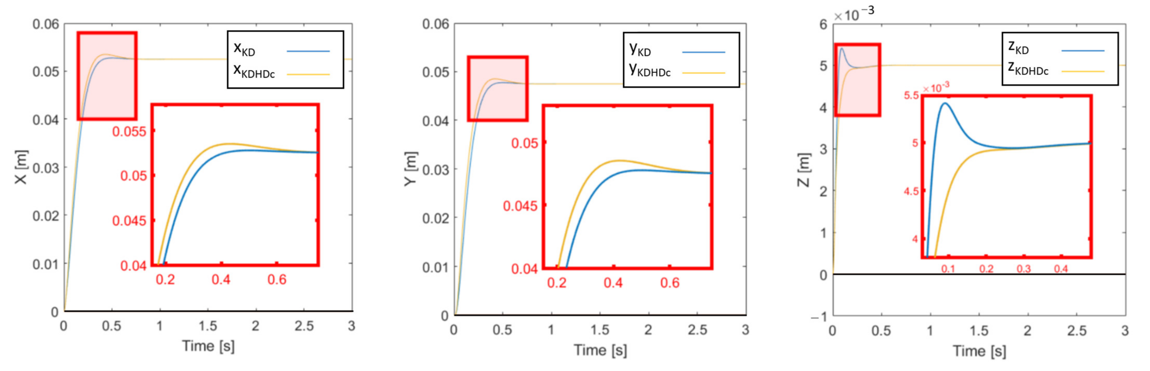
Figure 10 shows the simulation results with reference to the comparison number II (
ζKD = 1,
Table 2), in terms of external coordinates for the KD and KDHDc control laws.
The effectiveness of the KDHDc stiffness compensation is also validated in this case by the fact that the external coordinates tend to the same steady-state values of the KD control law. The steady-state displacement along
xW is slightly higher than the steady-state displacement
yW, while the steady-state displacement along
zW is much lower. This is coherent with the fact that the principal direction with lower stiffness is
xP, which is rotated by 45° around the
z-axis; therefore, considering only the
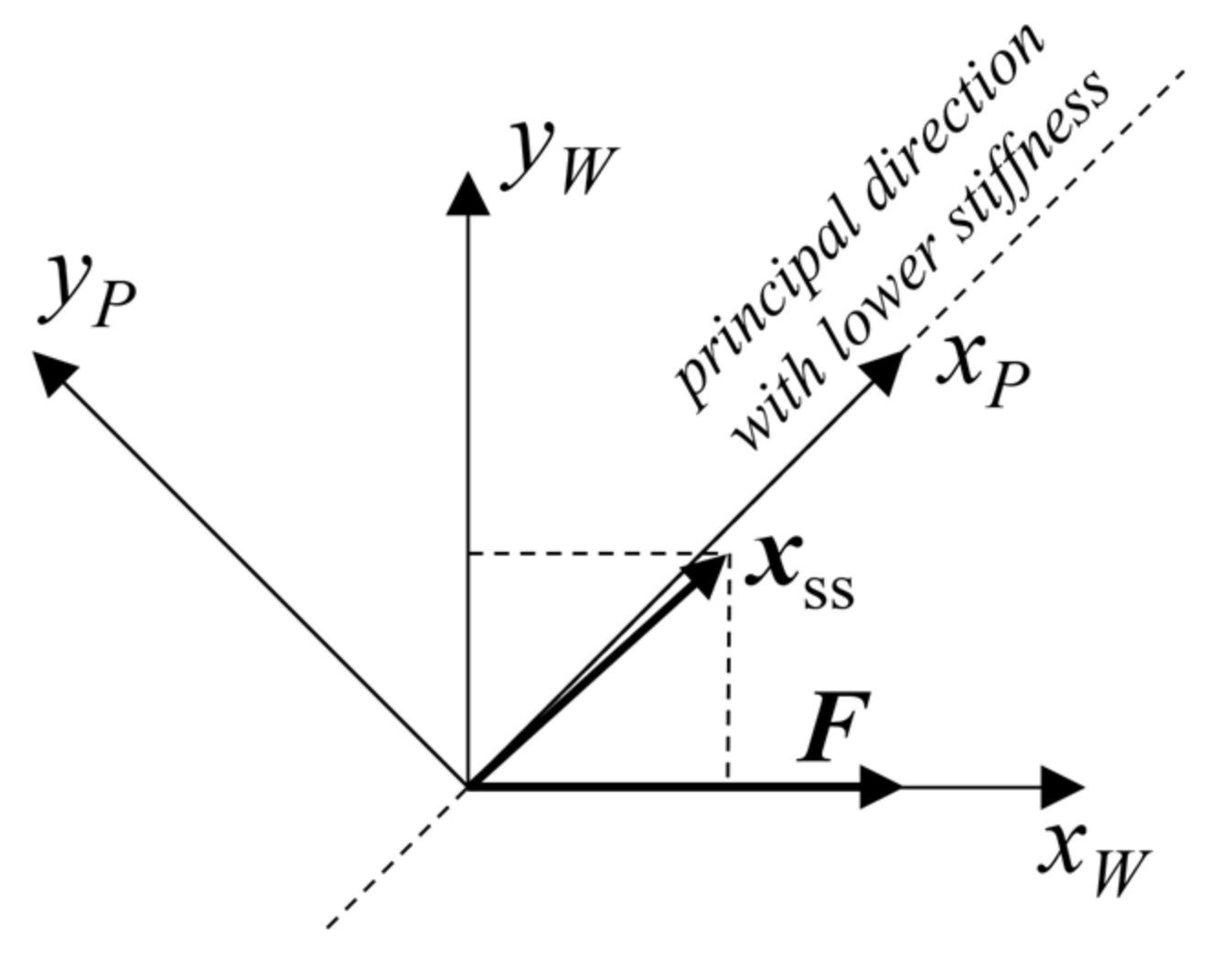
x-y plane (
Figure 11), a force along
xW causes a larger displacement along
xP with a positive direction, and a smaller displacement along
yP with a negative direction. This results, in the frame W, in a slightly higher displacement along
xW with respect to
yW. In this case study, the ratio between the stiffness along
xP and the ones along
yP and
zP is 1/20; imposing a lower ratio, the displacement would more precisely follow the desired compliance direction.
6. Conclusions
In this paper, an extension of classical impedance control (KD), with compliance defined by the stiffness (K) and damping (D) matrices, has been proposed and tested by multibody simulation on a 3-PUU parallel robot. This extension is based on fractional calculus, and in particular on the half-order derivative (derivative of order 1/2), adding a half-derivative damping defined by the matrix HD.
This work was inspired by the research about the PDD1/2 control scheme for SISO systems, which is a PD with the addition of the half-derivative term, and extended it to a particular class of MIMO systems, impedance-controlled robots. In this work, a PKM was considered, but the approach can also be applied to serial robots by using Equations (12) to (14).
This work is only a starting point, and the effects of the introduction of the half-derivative damping must be further investigated. However, it is possible to outline the following conclusions:
Even if applied to a nonlinear MIMO system, the introduction of the half-derivative term allows to tune the system behavior differently from a classical KD impedance control. The gains’ set used in the case study A attained a reduction of maximum actuation force and total control effort, but the system can be tuned differently in order to improve other performance indexes, exploiting the previous works on PDD1/2 control.
The addition of the half-derivative damping necessarily introduced, with the discrete-time implementation by a finite-order digital filter, an alteration to the stiffness of the impedance control in steady state, as shown by Equation (5) and
Figure 1. This hinders the capability of impedance control to regulate the contact force between the end-effector and the environment, which is the main scope of impedance control. To solve this issue, a stiffness-compensated KDHD impedance control algorithm (KDHDc) has been proposed (Equation (24)), and its effectiveness has been verified by simulation.
The saturation of the currents, and consequently of the actuation forces on the sliders, has not been taken into account to avoid the influence of an additional parameter, introducing a highly nonlinear effect and making the KD-KDHD comparison more complex. In any case, the simulations showed that the maximum actuation forces, with the considered control gains, were lower with the KDHD impedance control, so saturation cannot undermine the benefits of the proposed scheme.
In the future research, a systematic analysis of the influence of the control parameters of the KDHDc impedance control algorithm will be carried out in order to highlight the benefits of the proposed approach, also considering serial chains and robots with rotational mobility.


