
Robust Attitude Control of an Agile Aircraft Using Improved Q-Learning


Abstract
:1. Introduction
- (1)
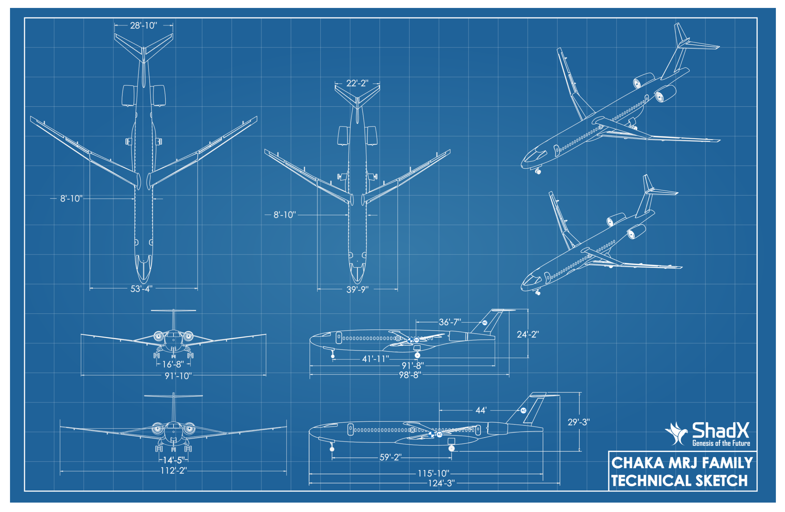
- Alongside the response to global aviation society demands, a TBW aircraft (Chaka 50) (Figure 1) with poor stability characteristics has been chosen for the attitude control problem;
- (2)
- It will be demonstrated that the proposed reward function is able to provide a robust control system even in low-stability and high-degree-of-freedom plants;
- (3)
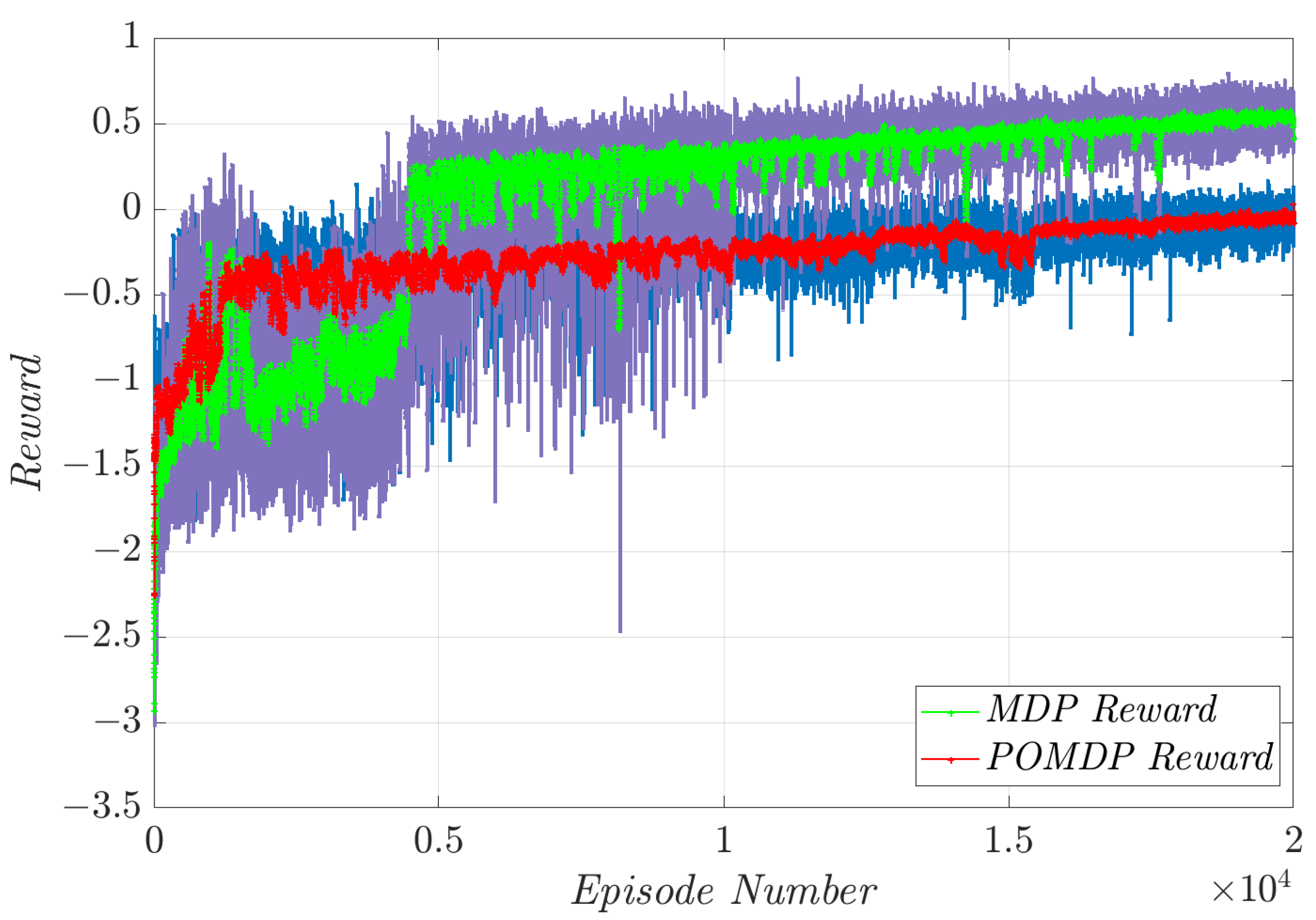
- The performance of the Q-learning controller will be evaluated in both MDP and POMDP problem definitions using different control criteria. Moreover, by proposing an effective Fuzzy Action Assignment (FAA) algorithm, continuous elevator commands could be generated using the discrete optimal Q-table (policy). Such a control approach illustrates well that the tabular Q-learning method can be a strong learning approach resulting in an effective controller for complex systems under uncertain conditions;
- (4)
- In order to prove the reliability and robustness of the proposed control method, it is examined under different flight conditions consisting of sensor measurement noises, atmospheric disturbances, actuator faults, and model uncertainties, while the training process is only performed for ideal flight conditions.
2. Modeling and Simulation
2.1. Atmospheric Disturbance and Sensor Measurement Noise
2.2. Elevator Fault
3. Attitude Control Using Q-Learning
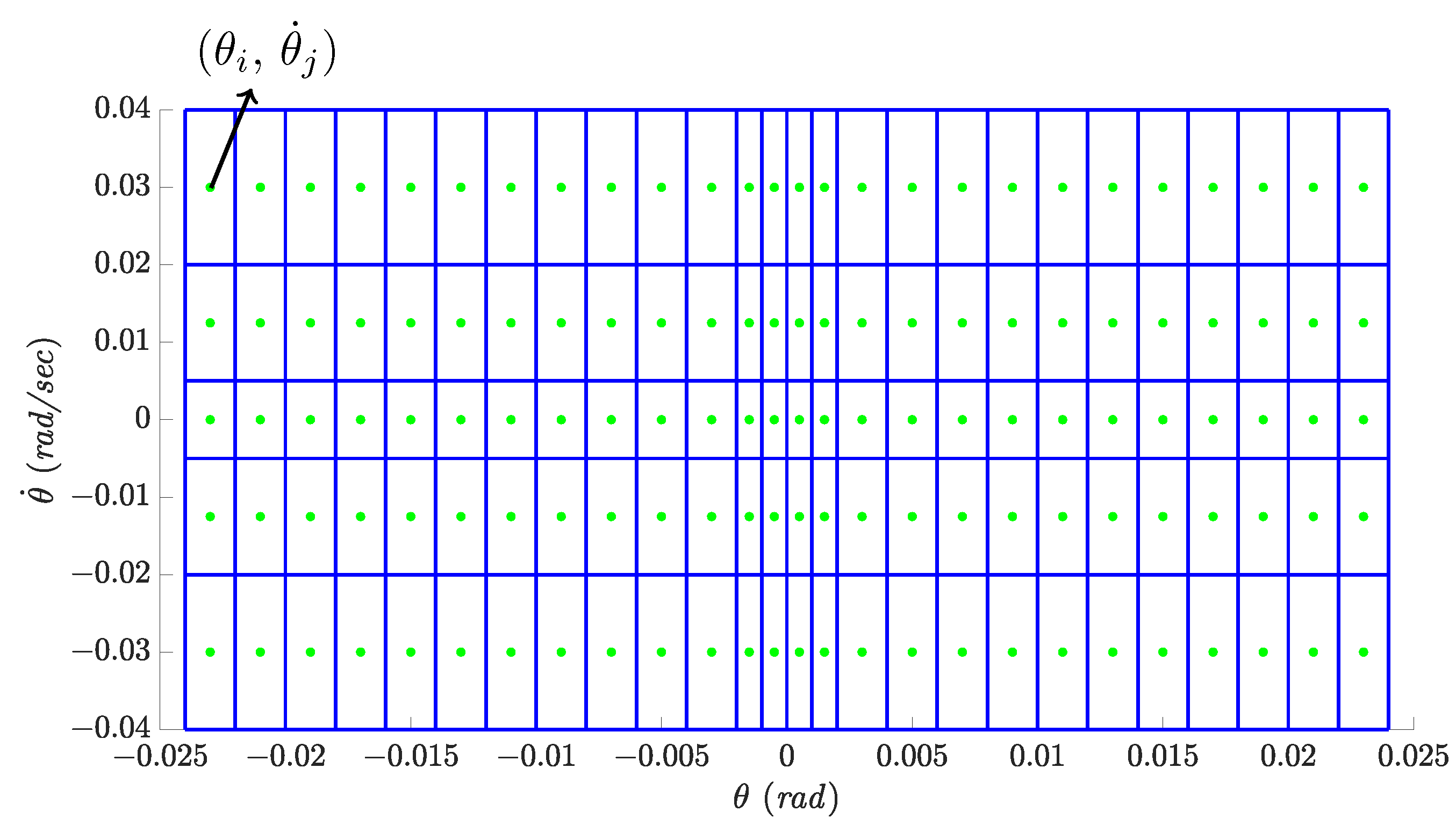
3.1. MDP and POMDP Definition in Attitude Control
3.2. Structure of Q-Learning Controller
| Algorithm 1: Q-learning Aircraft Attitude Controller |
 |
3.3. Reward Function and Action Space Definition
3.4. Structure of Fuzzy Action Assignment
| Algorithm 2: Q-learning controller improved by FAA scheme |
 |
4. Simulation Results and Discussion
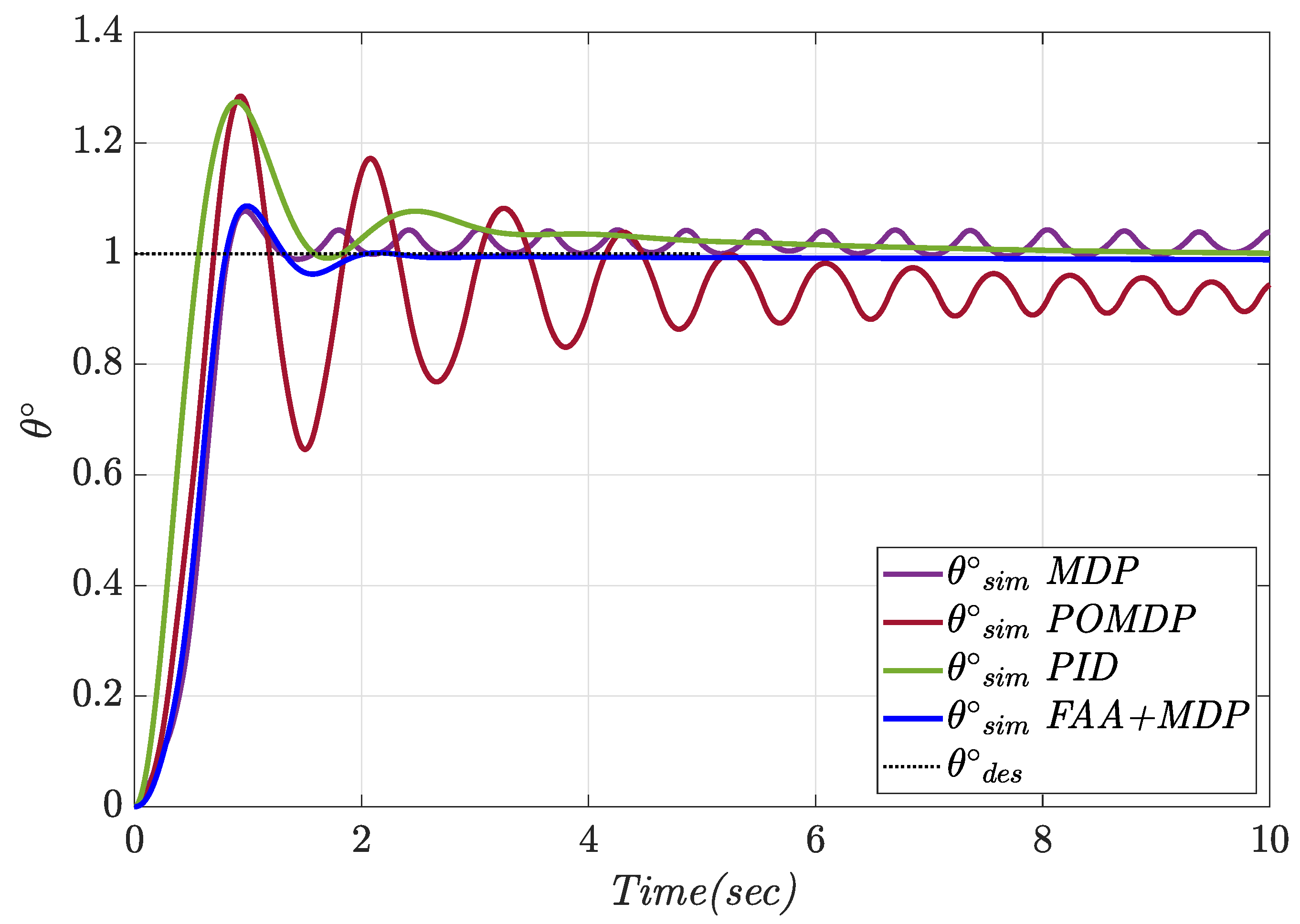
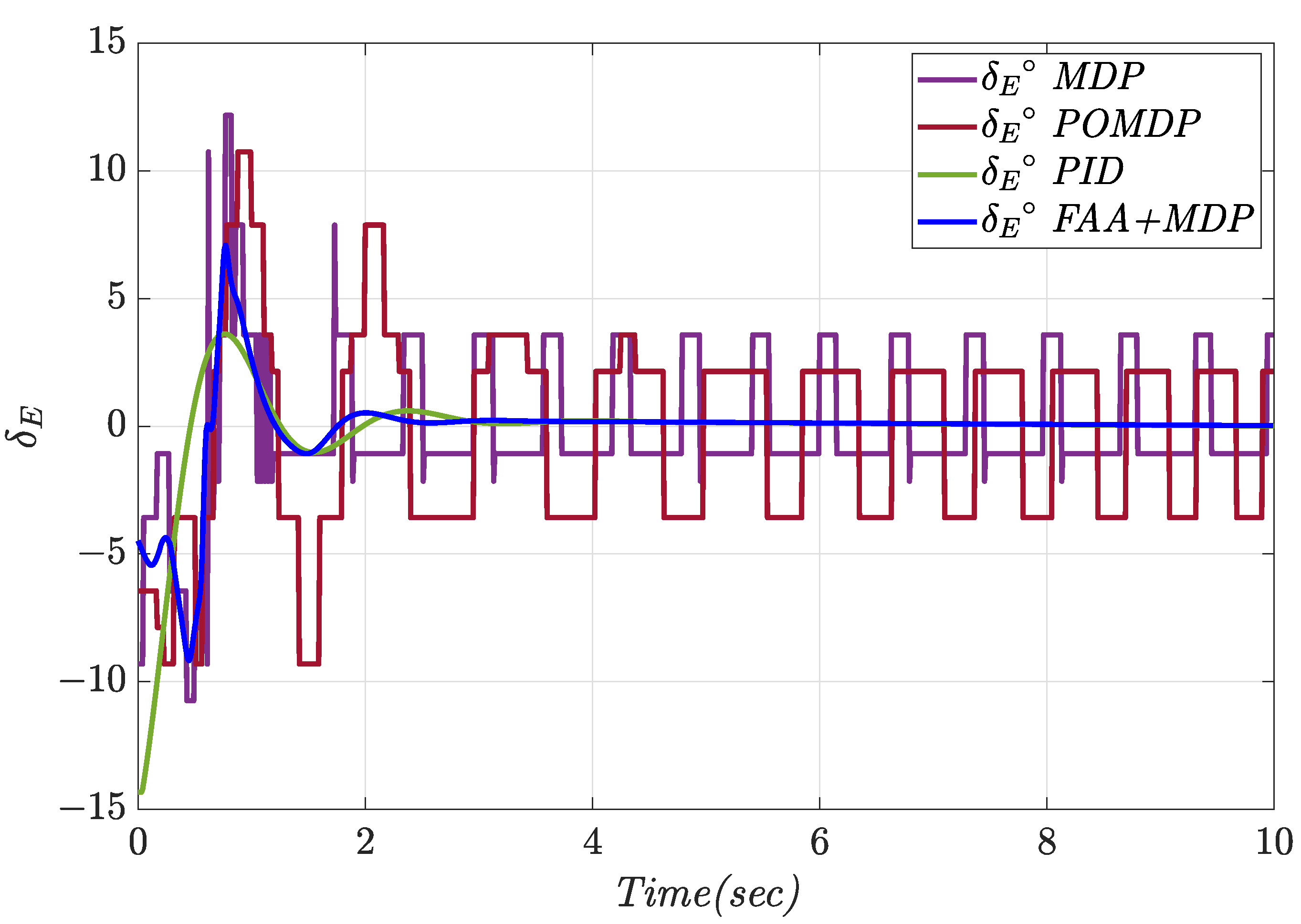
4.1. Constant Pitch Angle Tracking
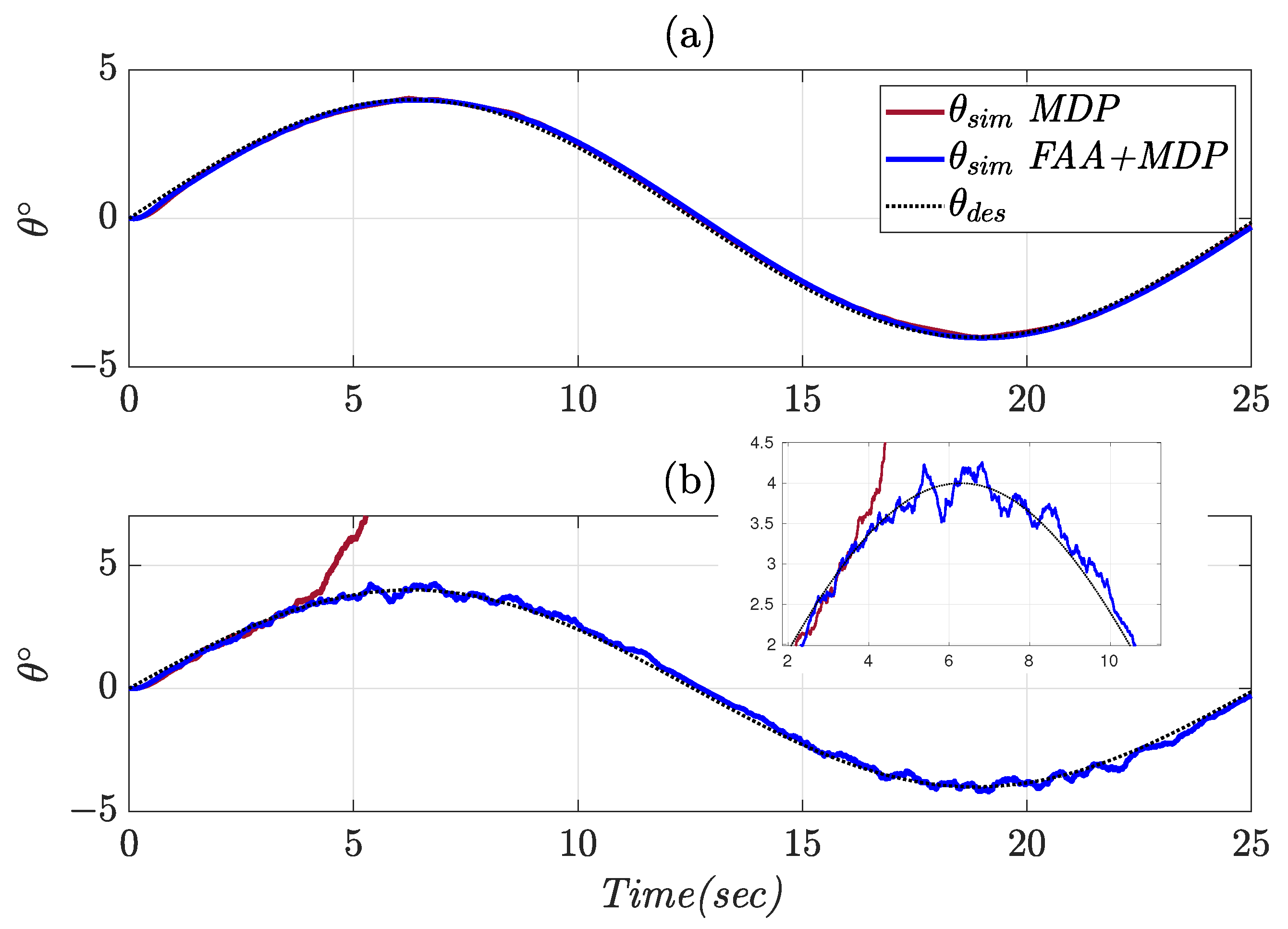
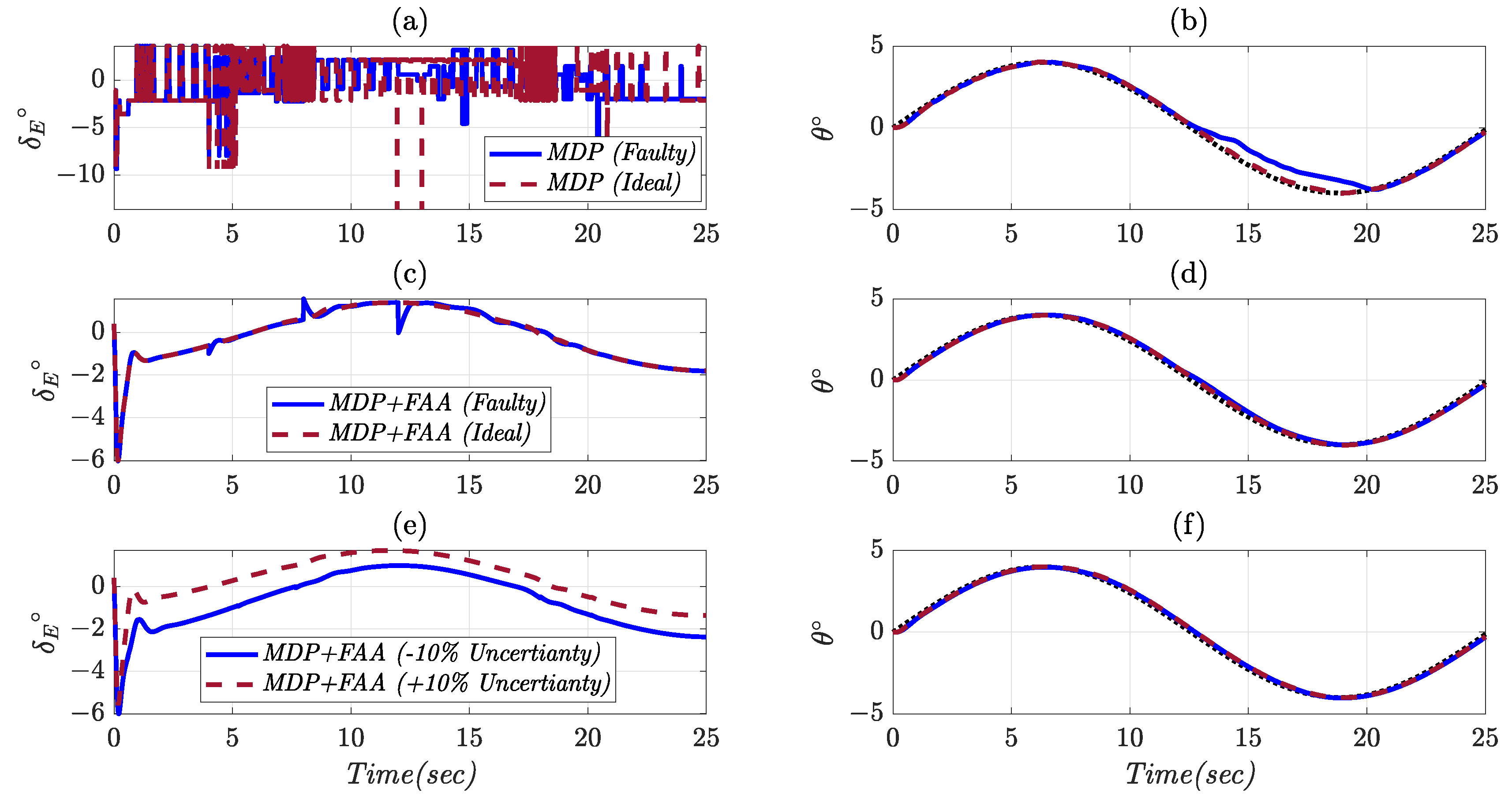
4.2. Variable Pitch Angle Tracking
5. Conclusions
Author Contributions
Funding
Data Availability Statement
Conflicts of Interest
Nomenclature
| Velocity components in body frame | |
| Angular velocity components in body frame | |
| Roll, pitch, and yaw angles | |
| Moments of inertia in body frame | |
| m | Mass of airplane |
| Aerodynamic force vector in body frame | |
| Engine thrust vector in body frame | |
| Aerodynamic moment vector | |
| Thrust moment vector in body frame | |
| g | Acceleration of gravity |
| D | Drag |
| L | Lift |
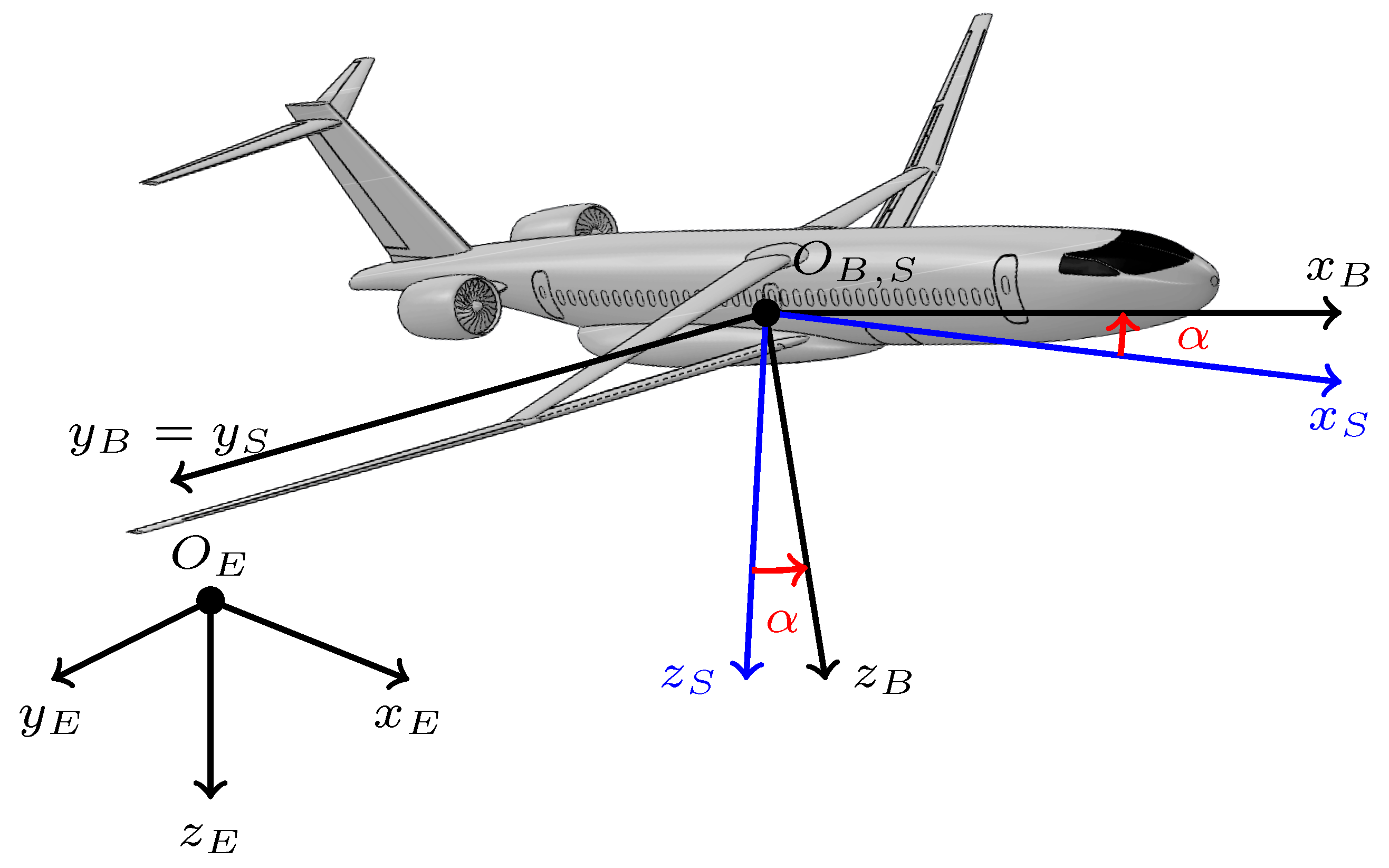
| Angle of attack | |
| Elevator deflection | |
| Airplane dynamic pressure | |
| Mean aerodynamic chord | |
| S | Wing Area |
| State-action value function | |
| R | Reward |
| Learning rate | |
| Proportional, integral, derivative coefficients of PID controller |
References
- Li, L.; Bai, J.; Qu, F. Multipoint Aerodynamic Shape Optimization of a Truss-Braced-Wing Aircraft. J. Aircr. 2022, 59, 1–16. [Google Scholar] [CrossRef]
- Sarode, V.S. Investigating Aerodynamic Coefficients and Stability Derivatives for Truss-Braced Wing Aircraft Using OpenVSP. Ph.D. Thesis, Virginia Tech, Blacksburg, VA, USA, 2022. [Google Scholar]
- Nguyen, N.T.; Xiong, J. Dynamic Aeroelastic Flight Dynamic Modeling of Mach 0.745 Transonic Truss-Braced Wing. In Proceedings of the AIAA SCITECH 2022 Forum, San Diego, CA, USA, 3–7 January 2022; p. 1325. [Google Scholar]
- Zavaree, S.; Zahmatkesh, M.; Eghbali, K.; Zahiremami, K.; Vaezi, E.; Madani, S.; Kariman, A.; Heidari, Z.; Mahmoudi, A.; Rassouli, F.; et al. Modern Regional Jet Family (Chaka: A High-Performance, Cost-Efficient, Semi-Conventional Regional Jet Family); AIAA: Reston, VA, USA, 2021; Available online: https://www.aiaa.org/docs/default-source/uploadedfiles/education-and-careers/university-students/design-competitions/winning-reports—2021-aircraft-design/2nd-place—graduate-team—sharif-university-of-technology.pdf?sfvrsn=41350e892 (accessed on 5 December 2022).
- Emami, S.A.; Castaldi, P.; Banazadeh, A. Neural network-based flight control systems: Present and future. Annu. Rev. Control 2022, 53, 97–137. [Google Scholar] [CrossRef]
- Xi, Z.; Wu, D.; Ni, W.; Ma, X. Energy-Optimized Trajectory Planning for Solar-Powered Aircraft in a Wind Field Using Reinforcement Learning. IEEE Access 2022, 10, 87715–87732. [Google Scholar] [CrossRef]
- Bøhn, E.; Coates, E.M.; Reinhardt, D.; Johansen, T.A. Data-Efficient Deep Reinforcement Learning for Attitude Control of Fixed-Wing UAVs: Field Experiments. arXiv 2021, arXiv:2111.04153. [Google Scholar]
- Yang, X.; Yang, X.; Deng, X. Horizontal trajectory control of stratospheric airships in wind field using Q-learning algorithm. Aerosp. Sci. Technol. 2020, 106, 106100. [Google Scholar] [CrossRef]
- Hu, W.; Gao, Z.; Quan, J.; Ma, X.; Xiong, J.; Zhang, W. Fixed-Wing Stalled Maneuver Control Technology Based on Deep Reinforcement Learning. In Proceedings of the 2022 IEEE 5th International Conference on Big Data and Artificial Intelligence (BDAI), Fuzhou, China, 8–10 July 2022; pp. 19–25. [Google Scholar]
- Xue, W.; Wu, H.; Ye, H.; Shao, S. An Improved Proximal Policy Optimization Method for Low-Level Control of a Quadrotor. Actuators 2022, 11, 105. [Google Scholar] [CrossRef]
- Wang, Z.; Li, H.; Wu, H.; Shen, F.; Lu, R. Design of Agent Training Environment for Aircraft Landing Guidance Based on Deep Reinforcement Learning. In Proceedings of the 2018 11th International Symposium on Computational Intelligence and Design (ISCID), Hangzhou, China, 8–9 December 2018; Volume 02, pp. 76–79. [Google Scholar] [CrossRef]
- Yuan, X.; Sun, Y.; Wang, Y.; Sun, C. Deterministic Policy Gradient with Advantage Function for Fixed Wing UAV Automatic Landing. In Proceedings of the 2019 Chinese Control Conference (CCC), Guangzhou, China, 27–30 July 2019; pp. 8305–8310. [Google Scholar] [CrossRef]
- Tang, C.; Lai, Y.C. Deep Reinforcement Learning Automatic Landing Control of Fixed-Wing Aircraft Using Deep Deterministic Policy Gradient. In Proceedings of the 2020 International Conference on Unmanned Aircraft Systems (ICUAS), Athens, Greece, 1–4 September 2020; pp. 1–9. [Google Scholar] [CrossRef]
- Dai, H.; Chen, P.; Yang, H. Fault-Tolerant Control of Skid Steering Vehicles Based on Meta-Reinforcement Learning with Situation Embedding. Actuators 2022, 11, 72. [Google Scholar] [CrossRef]
- Richter, D.J.; Natonski, L.; Shen, X.; Calix, R.A. Attitude Control for Fixed-Wing Aircraft Using Q-Learning. In Intelligent Human Computer Interaction; Kim, J.H., Singh, M., Khan, J., Tiwary, U.S., Sur, M., Singh, D., Eds.; Springer International Publishing: Cham, Swizerland, 2022; pp. 647–658. [Google Scholar]
- Watkins, C.J.; Dayan, P. Q-learning. Mach. Learn. 1992, 8, 279–292. [Google Scholar] [CrossRef]
- Glorennec, P.; Jouffe, L. Fuzzy Q-learning. In Proceedings of the 6th International Fuzzy Systems Conference, Barcelona, Spain, 5 July 1997; Volume 2, pp. 659–662. [Google Scholar] [CrossRef]
- Er, M.J.; Deng, C. Online tuning of fuzzy inference systems using dynamic fuzzy Q-learning. IEEE Trans. Syst. Man Cybern. Part B (Cybern.) 2004, 34, 1478–1489. [Google Scholar] [CrossRef] [PubMed]
- Napolitano, M.R. Aircraft Dynamics; Wiley: Hoboken, NJ, USA, 2012. [Google Scholar]
- Zipfel, P. Modeling and Simulation of Aerospace Vehicle Dynamics, 3rd ed.; AIAA: Reston, VA, USA, 2014. [Google Scholar]
- Wood, A.; Sydney, A.; Chin, P.; Thapa, B.; Ross, R. GymFG: A Framework with a Gym Interface for FlightGear. arXiv 2020, arXiv:2004.12481. [Google Scholar]
- Roskam, J. Airplane Flight Dynamics and Automatic Flight Controls; DARcorporation: Lawrence, KS, USA, 1998. [Google Scholar]
- Mil-f, V. 8785c: Flying Qualities of Piloted Airplanes; US Air Force: Washington, DC, USA, 1980; Volume 5. [Google Scholar]
- Frost, W.; Bowles, R.L. Wind shear terms in the equations of aircraft motion. J. Aircr. 1984, 21, 866–872. [Google Scholar] [CrossRef]
- Çetin, E. System identification and control of a fixed wing aircraft by using flight data obtained from x-plane flight simulator. Master’s Thesis, Middle East Technical University, Ankara, Turkey, 2018. [Google Scholar]
- Sutton, R.S.; Barto, A.G. Reinforcement Learning: An Introduction; MIT Press: Cambridge, MA, USA, 2018. [Google Scholar]
- Emami, S.A.; Banazadeh, A. Intelligent trajectory tracking of an aircraft in the presence of internal and external disturbances. Int. J. Robust Nonlinear Control 2019, 29, 5820–5844. [Google Scholar] [CrossRef]
- Emami, S.A.; Ahmadi, K.K.A. A self-organizing multi-model ensemble for identification of nonlinear time-varying dynamics of aerial vehicles. Proc. Inst. Mech. Eng. Part I J. Syst. Control. Eng. 2021, 235, 1164–1178. [Google Scholar] [CrossRef]


| Longitudinal Derivatives | Take-Off | Cruise | −10% Model Uncertainty | +10% Model Uncertainty |
|---|---|---|---|---|
| 0.0378 | 0.0338 | 0.0304 | 0.0371 | |
| 0.3203 | 0.3180 | 0.2862 | 0.3498 | |
| −0.07 | −0.061 | −0.054 | −0.067 | |
| 0.95 | 0.8930 | 0.8037 | 0.9823 | |
| 11.06 | 14.88 | 13.39 | 16.37 | |
| −12.18 | −11.84 | −10.65 | −13.02 | |
| 0.040 | 0.041 | 0.0369 | 0.0415 | |
| 0 | 0.081 | 0.0729 | 0.0891 | |
| 0 | −0.039 | −0.0351 | −0.0429 | |
| 0 | 0 | 0 | 0 | |
| 11.31 | 12.53 | 11.27 | 13.78 | |
| −40.25 | −40.69 | −36 | −44 | |
| 0.1550 | 0.1570 | 0.1413 | 0.1727 | |
| 0.96 | 0.78 | 0.702 | 0.858 | |
| −6.15 | −5.98 | −5.38 | −6.57 |
| Required Thrust () (lbs) | Angle of Attack () | Required Elevator () |
|---|---|---|
| 21,433.02 | 0.39 | −2.28 |
| Parameter | Value | Parameter | Value |
|---|---|---|---|
| Wing Area (m) | 43.42 | (kgm) | 378,056.535 |
| Mean Aerodynamic Chord (m) | 1.216 | (kgm) | 4,914,073.496 |
| Span (m) | 28 | (kgm) | 5,670,084.803 |
| Mass (kg) | 18,418.27 | (kgm) | 0 |
| Aircraft/ Roots | Short Period Roots | Phugoid Roots |
|---|---|---|
| Chaka 50 | ||
| Cessna 172 | ||
| Boeing N+3 |
| Parameter | Value |
|---|---|
| Epsilon() | |
| Alpha () | |
| Gamma () | |
| Episode number | 20,000 |
| (rad) | |
| (rad) | |
| 160 | |
| 300 | |
| Controller | Tracking Error (deg) | Control Effort (deg) | Overshoot (%) | Settling Time (s) |
|---|---|---|---|---|
| MDP | 0.071 | 2.11 | 7.38 | - |
| POMDP | 0.13 | 3.48 | 30.15 | - |
| PID | 0.066 | 0.69 | 27.42 | 5.44 |
| FAA + MDP | 0.057 | 0.69 | 8.20 | 1.76 |
| Controller | Flight Condition | Tracking Error (deg) | Control Effort (deg) |
|---|---|---|---|
| MDP | Ideal | 0.1081 | 2.224 |
| FAA + MDP | Ideal | 0.112 | 1.008 |
| MDP | Noise + Disturbance | 23.816 | 5.424 |
| FAA + MDP | Noise + Disturbance | 0.132 | 2.032 |
| MDP | Actuator Fault | 0.304 | 1.796 |
| FAA + MDP | Actuator Fault | 0.136 | 1.004 |
| FAA + MDP | −10% Uncertainty | 0.116 | 1.16 |
| FAA + MDP | +10% Uncertainty | 0.116 | 0.972 |
Publisher’s Note: MDPI stays neutral with regard to jurisdictional claims in published maps and institutional affiliations. |
© 2022 by the authors. Licensee MDPI, Basel, Switzerland. This article is an open access article distributed under the terms and conditions of the Creative Commons Attribution (CC BY) license (https://creativecommons.org/licenses/by/4.0/).
Share and Cite
Zahmatkesh, M.; Emami, S.A.; Banazadeh, A.; Castaldi, P. Robust Attitude Control of an Agile Aircraft Using Improved Q-Learning. Actuators 2022, 11, 374. https://doi.org/10.3390/act11120374
Zahmatkesh M, Emami SA, Banazadeh A, Castaldi P. Robust Attitude Control of an Agile Aircraft Using Improved Q-Learning. Actuators. 2022; 11(12):374. https://doi.org/10.3390/act11120374
Chicago/Turabian StyleZahmatkesh, Mohsen, Seyyed Ali Emami, Afshin Banazadeh, and Paolo Castaldi. 2022. "Robust Attitude Control of an Agile Aircraft Using Improved Q-Learning" Actuators 11, no. 12: 374. https://doi.org/10.3390/act11120374
APA StyleZahmatkesh, M., Emami, S. A., Banazadeh, A., & Castaldi, P. (2022). Robust Attitude Control of an Agile Aircraft Using Improved Q-Learning. Actuators, 11(12), 374. https://doi.org/10.3390/act11120374