Fixed-Time Incremental Neural Control for Manipulator Based on Composite Learning with Input Saturation

Abstract

In this paper, an adaptive incremental neural network (INN) fixed-time tracking control scheme based on composite learning is investigated for robot systems under input saturation. Firstly, by integrating the composite learning method into the INN to cope with the inevitable dynamic uncertainty, a novel adaptive updating law of NN weights is designed, which does not need to satisfy the stringent persistent excitation (PE) conditions. In addition, for the saturated input, differing from adding the auxiliary system, this paper introduces a hyperbolic tangent function to deal with the saturation nonlinearity by converting the asymmetric input constraints into the symmetric ones. Moreover, the fixed-time control approach and Lyapunov theory are combined to ensure that all the signals of the robot closed-loop control systems converge to a small neighborhood of the origin in a fixed time. Finally, numerical simulation results verify the effectiveness of the fixed-time control and composite learning algorithm.

1. Introduction

With the development of automation technology towards intelligent manufacturing, robots have been widely used in military rescue, intelligent assembly, human robot cooperation tasks, and other industrial manufacturing fields. On many occasions, robots and humans share the same workspace. If robot tasks are not performed accurately, unexpected accidents will occur. Therefore, how to accurately control the robots to perform the required tasks has always been an exceedingly important research direction [1,2,3]. Many scholars have proposed the model-based control schemes in which the inherent dynamics of the robot are fully known. However, in practice, due to the uncertainty of the environment and the coupling effect, it is difficult to determine the manipulator model and obtain the required control accuracy correctly and quickly. Thus, in recent years, a great deal of control schemes based on universal approximation such as neural networks (NNs) [4,5,6,7] and fuzzy logic systems (FLSs) [8,9,10] have emerged to deal with the unknown nonlinearity terms in the manipulator systems. If the network nodes were selected unreasonably, this would lead to insufficient learning of the nonlinear terms and the degradation of approximation performance, which was the common weakness in the above-mentioned NN approximation. An effective way to settle this issue is to dynamically increase the number of nodes, which is called the INN [11]. No matter whether the NN or INN, it should be pointed out that the network weight converges to the real value when the sufficient condition for accurate approximation is established, and the PE condition is an important condition to ensure the convergence of estimation [12]. The PE condition is difficult to achieve, so it is often not feasible in practical systems. It is worth emphasizing that the partial PE condition proposed in [13] relaxed the traditional PE, and it was pointed out that any recursive NN input trajectory of the radial basis function neural network (RBFNN) defined in a local regular lattice can be partially activated. In the works [14,15,16,17], this idea was utilized in the adaptive control design of nonlinear systems such as a manipulator, to ensure the stability and realize the convergence of the NN weights. Based on the above discussion, how to solve the problem of insufficient learning caused by improper node selection on the basis of relaxing the strict PE condition still needs to be further discussed.

On the other hand, during the task of a manipulator, the input control torque cannot exceed a certain upper limit value due to the inevitable constraints of electromechanical failure or mechanical structure change. If the torque required by the controller exceeds the torque provided by the actuator, unpredictable mechanical faults may occur, thereby damaging the system performance. Hence, it is a meaningful work to investigate the input saturation [18,19,20,21,22,23,24] for practical nonlinear systems. For uncertain nonlinear systems, considering the effect of input saturations, the authors in [18,19], by constructing an auxiliary system, developed two effective control schemes to restrain them. Subsequently, the works in [22,23,24] extended the above methods to robotic manipulators [22], ships [23], and suspension systems [24] and proposed several control schemes that can suppress the adverse effects of saturation on the actual systems. Obviously, these schemes compensated the saturations’ nonlinearity by introducing an auxiliary system, yet the auxiliary system intensified the complexity of the system structure to a certain extent, expanded the amount of calculation, and may also lead to chattering. In order to amend these flaws, the works in [20,21] designed a hyperbolic tangent function to approximate the saturation nonlinearity for symmetric input constraints, which alleviated the vibration and large amount of calculation caused by the auxiliary system. Nevertheless, it must be emphasized that the above work did not consider the asymmetric saturation of the actuators or require the convergence time of the controlled system. To a certain extent, rapid convergence will lead to the increase of the vibration amplitude. Therefore, under the constraint of input nonlinearity, it is hard to obtain stability and good error convergence, which inspired our research.

In order to achieve high accuracy and fast convergence, the control approach of finite-time convergence is a preferred solution. The pioneering work [25] introduced the concept of finite-time stability and proved that it has high-level robustness and faster transient response. Subsequently, many scholars have followed this work, and many constructive works have emerged [26,27,28,29]. The work [26] presented a smooth finite-time control scheme of strict feedback nonlinear systems, and the work [27] investigated the issue of finite-time for nonlinear systems with unmeasurable states through a quantized feedback control strategy. The research [25,26,27,28,29] limited the convergence time to a range by finite-time control, but all relied on the initial state of the system. For the sake of breaking these restrictions, the authors in [30] proposed a fixed-time control scheme, which is independent of the initial conditions and can be adjusted by the controller parameters. To this end, a large number of adaptive intelligent control algorithms have been developed [31,32,33,34,35]. By applying universal barrier functions, a fixed-time control with symmetric constraints for MIMO uncertain systems was studied in [31]. In [32], the observer-based fixed-time tracking control problem of SISO nonlinear systems was considered. In [33,34], the fixed-time method was extended to multiagent systems and a flexible robotic manipulator. In [35], the authors developed fixed-time control with distrubance for manipulator system, and the work of this paper extends [35] and introduces composite learning approach on the fram work of the NN fixed-time theory.

Inspired by the above discussions, this paper proposes an adaptive INN fixed-time tracking control scheme based on composite learning for the manipulator system under saturated input. The main contributions are as follows:

• A new INN adaptive algorithm based on the composite learning technique is designed. By dynamically generating network nodes and introducing some persistence conditions to adapt to the NN weights, the estimation error information can be properly integrated into the adaptive law, and the estimation performance is improved on the basis of relaxing the traditional PE conditions. Even though the works [14,15,16,17] studied composite learning control, they did not consider dynamically activating network nodes to adjust the NN input, let alone ensuring that the estimation error converged in a fixed time.
• In the framework of the backstepping composite learning approach, the challenge of devising a fixed-time controller with asymmetric actuator saturation of the manipulator system is effectively tackled. Although the authors in [18,19,22,23,24] considered the problem of actuator input saturation, they all solved symmetric saturation by introducing auxiliary systems, which is not tenable for the asymmetric scenario. Instead, this paper not only proposes a feasible asymmetric saturation control scheme, but also ensures fixed-time convergence under the composite learning framework.

The rest of this paper is structured as follows. In Section 2, the system description and some useful lemmas are introduced. Section 3 shows the radial basis function NN and the INN. Section 4 introduces how to design the INN controller based on composite learning in the presence of input saturation and presents the stability analysis. The proposed control scheme in this paper is validated by the simulation in Section 5. Finally, Section 6 gives the conclusion of this paper.

2. System Description

The dynamic model of a manipulator with n degrees of freedom can be described as:

$$H\left(\theta \right)\ddot{\theta }+C(\dot{\theta },\theta )\dot{\theta }+G\left(\theta \right)=\tau$$

(1)

where $\theta \in {\mathbb{R}}^n$ represents the joint position angle vector, $H\left(\theta \right)\in {\mathbb{R}}^{n\times n}$ represents the inertia matrix, $C(\dot{\theta },\theta )\in {\mathbb{R}}^{n\times n}$ represents the Coriolis matrix, $G\left(\theta \right)\in {\mathbb{R}}^n$ represents the gravity, and $\tau \in {\mathbb{R}}^n$ represents the control torque and satisfies

$${\tau }_i=\left\{\begin{array}{c}{\tau }_{imax},u_i>u_{imax}\hfill \\ f_{ri}\left(u_i\right),0\le u_i\le u_{imax}\hfill \\ f_{li}\left(u_i\right),-u_{imin}\le u_i\le 0\hfill \\ -{\tau }_{imin},u_i<-u_{imin}\hfill \end{array}\right.$$

(2)

where $u_i(i=1,\dots ,n)$ is the i-th element of the control law $u={[u_1,u_2,\dots ,u_n]}^T$. ${\tau }_{max}={[{\tau }_{1max},\dots ,{\tau }_{nmax}]}^T$, ${\tau }_{min}={[{\tau }_{1min},\dots ,{\tau }_{nmin}]}^T$, $u_{max}={[u_{1max},\dots ,u_{nmax}]}^T$, and $u_{min}={[u_{1min},\dots ,u_{nmin}]}^T$ are the known saturation parameters; nonlinear functions $f_{ri}\left(u_i\right)$ and $f_{li}\left(u_i\right)$ are unknown, but smoothly continuous; $f_{ri}\left(0\right)=f_{li}\left(0\right)=0$ and the assumption that $v_{ri0}\le {\dot{f}}_{ri}\left(u_i\right)\le v_{ri1}$, $v_{li0}\le {\dot{f}}_{li}\left(u_i\right)\le v_{li1}$ are satisfied in $u_i\in [0,u_{imax}]$ and $u_i\in [-u_{imin},0]$, respectively, where $v_{ri0}$, $v_{ri1}$, $v_{li0}$, and $v_{li1}$ are positive constants.

The manipulator has the following two commonly used properties.

Property 1

([10]). For any θ, $\dot{\theta }\in {\mathbb{R}}^n$, H, C, and G are bounded and their first derivatives are available.

Property 2

([10]). $\dot{H}-2C$ is an antisymmetric matrix, which means, for any $z\in {\mathbb{R}}^n$, $z^T$ $(\dot{H}-2C)z=0$ are established.

Lemma 1

([31]). If a positive Lyapunov function $V\left(x\right)$ satisfies: $\dot{V}<-p{V}^{\alpha }-q{V}^{\beta }+h$, where $p>0$, $q>0$, $h>0$, $0<\alpha <1$, and $\beta >1$, then the system $\dot{x}=f(x,t)$ is considered to be stable in fixed-time, whose solution will converge to a compact set $\Omega =\left\{x\right|V\le min\left(\right[h/$${\left(p(1-\gamma )\right)]}^{1/\alpha },{[h/\left(q(1-\gamma )\right)]}^{1/\beta }\left)\right\}$, where $0<\gamma <1$, and the convergence time of the system satisfies: $T\le T_{max}=\frac{1}{p\gamma (1-\alpha )}+\frac{1}{q\gamma (\beta -1)}$.

Lemma 2

([31,33]). For any $x_i\in \mathbb{R}$, we have

$$\sum _{i=1}^n{\left|x_i\right|}^r\ge {\left(\sum _{i=1}^n\left|x_i\right|\right)}^r,if0<r\le 1$$

(3)

$$\sum _{i=1}^n{\left|x_i\right|}^r\ge n^{1-r}{\left(\sum _{x=1}^n\left|x_i\right|\right)}^r,ifr>1$$

(4)

Lemma 3

([16]). The vector ${\xi }_2$ is not used, then its estimate value can be obtained according to the following second-order filter:

$$\begin{array}{c}\hfill \left\{\begin{array}{c}{\dot{\widehat{\xi }}}_1={\widehat{\xi }}_2\hfill \\ {\dot{\widehat{\xi }}}_2=w^2({\xi }_1-{\widehat{\xi }}_1)-\zeta w{\widehat{\xi }}_2\hfill \end{array}\right.\end{array}$$

(5)

where ${\widehat{\xi }}_1$ and ${\widehat{\xi }}_2$ are estimates of ${\xi }_1$ and ${\xi }_2$, respectively. Note that with the frequency w fit low enough, the estimation error of ${\xi }_2$ is small enough to make ${\widehat{\xi }}_2\approx {\xi }_2$.

Definition 1

([13]). For an n-dimensional bounded column vector $\Phi \left(t\right)$, if there are positive constants $a_1$, $a_2$, and $t_0$ such that $a_1\mathit{I}\le {\int }_{t_0}^{t_0+\Delta t}\Phi \left(u\right){\Phi }^T\left(u\right)du\le a_2\mathit{I}$ is valid for arbitrary time interval $\Delta t$, then the bounded signal $\Phi \left(t\right)$ is called PE.

3. Radial Basis Function NN Approximator

The RBFNN has a strong nonlinear approximation ability. As long as there are enough nodes, any nonlinear term can be approximated with any accuracy. However, due to the limited number of nodes in practical applications, there will be an approximation error. The expression of the RBFNN approximating the nonlinear term is

$$Y\left(x\right)=W^T\Phi \left(x\right)+ϵ\left(x\right)$$

(6)

where $W\in {\mathbb{R}}^{n\times k}$ denotes the network weight, $\Phi \left(x\right)\in {\mathbb{R}}^k$ denotes the regression vector, $ϵ\left(x\right)\in {\mathbb{R}}^n$ denotes the approximation error, $x\in {\mathbb{R}}^m$ denotes the input vector of the network, n denotes the dimension of the nonlinear term to be estimated, k denotes the number of nodes in the neural network, and m denotes the dimension of the network input vector.

The Gaussian function is the most commonly used basis function in the RBFNN because of its simple form and being differentiable at any order, and its expression is as follows:

$${\Phi }_i\left(x\right)=exp[\frac{-{(x-{\mu }_i)}^T(x-{\mu }_i)}{{\sigma }_i^2}],i=1,\cdots ,k$$

(7)

where ${\mu }_i\in {\mathbb{R}}^m$ denotes the i-th node and ${\sigma }_i\in {\mathbb{R}}^{+}$ denotes the standard deviation.

In order to overcome the shortcomings of the inaccurate nodes manually set in advance, the method of incremental learning [11] to generate nodes is introduced, and the node addition process is shown in Figure 1. Firstly, the initial state of the system is set to the first node of the network, i.e.,

$$\mu \left(t_0\right)=x$$

(8)

In the following process, the network will decide whether to generate nodes according to the distance between the current input and the node set. After each sampling period T, the node set of the network is

$$\mu (t+T)=\left\{\begin{array}{ll}[\mu \left(t\right),{\mu }_{new}],& dis>\epsilon \\ \mu \left(t\right),& dis\le \epsilon \end{array}\right.$$

(9)

where $\mu \left(t\right)\in {\mathbb{R}}^{m\times k}$ denotes the node set of the network at time t, ${\mu }_{new}\in {\mathbb{R}}^{m\times 1}$ indicates the newly generated node, while $\mu (t+T)$ denotes the node set at time $t+T$. $dis$ denotes the Euclidean distance between the network input and node set, whose calculation formula is shown as (10), and $\epsilon$ is the distance threshold parameter to be designed.

$$dis=∥x-{\overline{\mu }}_{min}∥$$

(10)

where ${\overline{\mu }}_{min}$ represents the weighted average node of the neural network, which is obtained according to the weighted average of b nodes closest to the current input vector, i.e.,

$${\overline{\mu }}_{min}=\frac{{\sum }_{i=1}^{b}arg{min}_{\mu }\left\{\left|\right|x-{\mu }_i\left|\right|\right\}}{b}$$

(11)

Finally, the newly generated nodes of the network are

$${\mu }_{new}={\overline{\mu }}_{min}+\delta (x-{\overline{\mu }}_{min})$$

(12)

where $\delta >0$ is the parameter to be designed.

From the above process, it is not difficult to find that, compared with the traditional neural network, the neural network using incremental learning has a significant advantage in that it can ensure that the input is always in the compact domain of the neural network, enabling the maximum activation of the nodes. Since the degree of node activation depends on the Euclidean distance between the current input and the nodes and the nodes of the incremental neural network are generated according to the real-time input, when the current input is not in the network compact domain, the nodes will be automatically added to expand the compact domain, so the effectiveness of the incremental neural network can be better guaranteed. In contrast, the nodes in the traditional NN need to be set up artificially; when the prior knowledge of the complex system is not accurate, the designed node set is far away from the input of the system and cannot be activated effectively, which will lead to a significant reduction in the approximation performance of the network. We call the RBFNN with incremental learning the IRBFNN.

4. Controller Design and Stability Analysis

4.1. Controller Design

The proposed control scheme is shown in Figure 2. Let $z_1=\theta$ and $z_2=\dot{\theta }$; the dynamic equation of the system (1) can be rewritten as

$$H{\dot{z}}_2+C{z}_2+G=\tau$$

(13)

The state space equation of the manipulator can be sorted out as

$$\begin{array}{c}\hfill {\dot{z}}_1=z_2,{\dot{z}}_2=H^{-1}(\tau -C{z}_2-G)\end{array}$$

(14)

Thus, define the error signal of the system as

$$\begin{array}{c}\hfill {\tilde{z}}_1=z_1-{\theta }_d,{\tilde{z}}_2=z_2-z_{2d}\end{array}$$

(15)

where ${\theta }_d\in {\mathbb{R}}^n$ denotes the desired joint position and $z_{2d}\in {\mathbb{R}}^n$ denotes the virtual control law to be designed later.

The dynamic error equation of the system can be obtained as

$$H{\dot{\tilde{z}}}_2+C{\tilde{z}}_2=\tau -H{\dot{z}}_{2d}-C{z}_{2d}-G$$

(16)

According to the backstepping control method and the theory of fixed-time stability, design the virtual control law $z_{2d}$ as

$$z_{2d}=-K_{12}{\tilde{z}}_1-K_{12}\sum _{i=1}^n{w}_i\left({\tilde{z}}_{1,i}\right)-K_{13}Si{g}^{\beta }\left({\tilde{z}}_1\right)+{\dot{\theta }}_d$$

(17)

In order to ensure that $z_{2d}$ and its derivate are both continuous, the nonlinear function $w_i\left({\tilde{z}}_{1,i}\right)$ is designed as

$$w_i\left({\tilde{z}}_{1,i}\right)=\left\{\begin{array}{ll}Si{g}^{\alpha }\left({\tilde{z}}_{1,i}\right),& |{\tilde{z}}_{1,i}|\ge \vartheta \\ a_1{\tilde{z}}_{1,i}+a_2{\tilde{z}}_{1,i}^3,& |{\tilde{z}}_{1,i}|<\vartheta \end{array}\right.$$

(18)

where $\vartheta$ is a small constant, $Si{g}^c(.)=sign(.){|.|}^c$.

Using the IRBFNN to estimate the unknown model of the system, we obtain

$$Y\left(x\right)=W^T\Phi \left(x\right)+ϵ\left(x\right)=-H{\dot{z}}_{2d}-C{z}_{2d}-G$$

(19)

where $x=[z_1,z_2,z_{2d}]\in {\mathbb{R}}^{3n\times 1}$ is the input of the IRBFNN and $Y\left(x\right)\in {\mathbb{R}}^{n\times 1}$, $W\in {\mathbb{R}}^{k\times n}$, $\Phi \left(x\right)\in {\mathbb{R}}^{k\times 1}$, and $ϵ\left(x\right)\in {\mathbb{R}}^{n\times 1}$ represent the item to be estimated, the ideal weight, the regression vector, and the approximation error, respectively. k is the number of nodes of the IRBFNN, and $\left|\right|ϵ\left(x\right)\left|\right|\le \overline{ϵ}$. Thus, the dynamic error equation can be rewritten as

$$H{\dot{\tilde{z}}}_2+C{\tilde{z}}_2=\tau +W^T\Phi \left(x\right)+ϵ\left(x\right)$$

(20)

Define the estimated error $\tilde{W}$ of the network weight as

$$\tilde{W}=\widehat{W}-W$$

(21)

where $\widehat{W}$ is an estimate of the ideal network weight W.

In order to make the network weights converge in a fixed time without the strict PE condition, we designed the weight update law with composite learning technology [16]. Firstly, the error of the IRBFNN is defined as:

$$E_i\left(t\right)=B\left(t\right){\widehat{W}}_i-D_i\left(t\right),i=1,2,\dots ,n$$

(22)

where ${\widehat{W}}_i\left(t\right)\in {\mathbb{R}}^{k\times 1}$ represents the estimated network weight of the i-th joint and $E_i\left(t\right)\in {\mathbb{R}}^{k\times 1}$ is the corresponding network estimation error, and the auxiliary terms $B\left(t\right)\in {\mathbb{R}}^{k\times k}$ and $D_i\left(t\right)\in {\mathbb{R}}^{k\times 1}$ are defined as follows:

$$\begin{array}{c}\hfill \left\{\begin{array}{c}B\left(t\right)={\int }_0^t{e}^{-r(t-u)}\Phi \left(x\right){\Phi }^T\left(x\right)du\hfill \\ D_i\left(t\right)={\int }_0^t{e}^{-r(t-u)}\Phi \left(x\right)(W_i^T\Phi \left(x\right)+{ϵ}_i\left(x\right))du\hfill \end{array}\right.\end{array}$$

(23)

where $B\left(t\right)\in {\mathbb{R}}^{k\times k}$ is a symmetric matrix, and $B\left(t\right)=B^T\left(t\right)$.

Combining (23) and (21), the estimation error of the network (22) can be further arranged as

$$\begin{array}{cc}\hfill E_i=& B{\widehat{W}}_i-D_i\hfill \\ \hfill =& {\int }_0^t{e}^{-r(t-u)}\Phi \left(x\right)({\Phi }^T\left(x\right)({\widehat{W}}_i-W_i)-{ϵ}_i\left(x\right))du\hfill \\ \hfill =& B{\tilde{W}}_i+{\Psi }_i\hfill \end{array}$$

(24)

where ${\Psi }_i=-{\int }_0^t{e}^{-r(t-u)}\Phi \left(x\right){ϵ}_i\left(x\right)du$ and ${\Psi }_i$ is bounded. In (24), $B{\tilde{W}}_i$ corresponds to the estimation error of the network weight and ${\Psi }_i$ corresponds to the approximation error, so $E_i$ corresponds to the total error of the IRBFNN.

To calculate $W_i^T\Phi \left(x\right)+{ϵ}_i\left(x\right)$ in Equation (23), from Equations (13) and (19), we can obtain

$$W_i^T\Phi \left(x\right)+{ϵ}_i\left(x\right)={\tau }_i{\phi }_i$$

(25)

$${\phi }_i={\left[\begin{array}{c}{\dot{\tilde{z}}}_{2,i}+{\dot{z}}_{2d,i}\\ {\tilde{z}}_{2,i}+z_{2d,i}\\ 1\end{array}\right]}^{†}\left[\begin{array}{c}-{\dot{\tilde{z}}}_{2d,i}\\ -z_{2d,i}\\ -1\end{array}\right]$$

(26)

where ${[·]}^{†}$ denotes the pseudo inverse of a vector. Since $z_{2,i}={\ddot{\theta }}_i$ is the angular acceleration of the manipulator and cannot be obtained directly, its estimated value is obtained through the second-order filter shown in Lemma 3, that is

$${\widehat{\phi }}_i={\left[\begin{array}{c}{\widehat{\dot{z}}}_{2,i}+{\dot{z}}_{2d,i}\\ z_{2,i}+z_{2d,i}\\ 1\end{array}\right]}^{†}\left[\begin{array}{c}-{\dot{z}}_{2d,i}\\ -z_{2d,i}\\ -1\end{array}\right]$$

(27)

Then, the expression of $D_i\left(t\right)$ in Equation (23) can be further arranged as

$$D_i\left(t\right)={\int }_0^t{e}^{-r(t-u)}\Phi \left(x\right){\tau }_i{\widehat{\phi }}_{i}du$$

(28)

Obviously, the expression (23) is a solution for the system of differential Equation (29), so the update laws of the auxiliary terms B, D are set as:

$$\begin{array}{c}\hfill \left\{\begin{array}{c}\dot{B}=-rB+\Phi \left(x\right){\Phi }^T\left(x\right)\hfill \\ {\dot{D}}_i=-r{D}_i+\Phi \left(x\right){\tau }_i{\widehat{\phi }}_i\hfill \end{array}\right.\end{array}$$

(29)

Based on the composite learning approach, design ${\dot{\widehat{W}}}_i$ by the IRBFNN, as shown in (30):

$${\dot{\widehat{W}}}_i={\Gamma }_i^{-1}(\Phi \left(x\right){\tilde{z}}_{2,i}-K_{32,i}Si{g}^{\alpha }\left(E_i\right)-K_{33,i}Si{g}^{\beta }\left(E_i\right))$$

(30)

where ${\Gamma }_i\in {\mathbb{R}}^{k\times k}$, $K_{32,i}\in {\mathbb{R}}^{k\times k}$, and $K_{33,i}\in {\mathbb{R}}^{k\times k}$ are all full-rank diagonal constant matrices and their elements are all positive.

Remark 1.

It is not difficult to find that the weight composite learning law in the Formula (30) combines the position tracking error signal of the current system with the total error signal of the IRBFNN. The idea is to ensure the convergence of the weight by using the feedback effect of the historical error generated by the system and the updating of the weight. It should be noted that, compared with the existing results, the composite learning law designed by us can guarantee not only the weight convergence, but also convergences at a fixed time.

In order to satisfy the input saturation effect of the actuator, introduce the variable $\Xi$ to assist the torque design; one has

$$\Xi =diag[{\overline{\tau }}_i/{\overline{u}}_i],i=1,2,\cdots ,n$$

(31)

where $diag[·]$ denotes a diagonal matrix, ${\overline{\tau }}_i$ represents the upper limit of the torque that the actuator can accept, while ${\overline{u}}_i$ represents the parameter related to the expected maximum control law, and

$$\begin{array}{c}\hfill \left\{\begin{array}{c}{\overline{\tau }}_i={\tau }_{imax},{\overline{u}}_i=u_{imax},{\tau }_{imax}/u_{imax}\ge {\tau }_{imin}/u_{imin}\hfill \\ {\overline{\tau }}_i={\tau }_{imin},{\overline{u}}_i=u_{imin},{\tau }_{imax}/u_{imax}<{\tau }_{imin}/u_{imin}\hfill \end{array}\right.\end{array}$$

(32)

According to (20), we can obtain

$${\dot{\tilde{z}}}_2=H^{-1}(\Xi {\Xi }^{-1}\tau +W^T\Phi \left(x\right)+ϵ)-H^{-1}C{\tilde{z}}_2$$

(33)

In the proposed controller, the relation between the actual control torque $\tau$ and the designed control law u is as follows:

$$\tau =\chi \left(u\right)+\Delta \tau$$

(34)

where $\Delta \tau$ represents the difference between the actual input saturation effect curve and the ideal value and the assumption that $|\Delta \tau |\le \Delta \overline{\tau }$ and $\chi \left(u\right)$ represents the conversion value of the control law u after the saturation effect. Use the hyperbolic tangent function to solve the input saturation effect, that is

$$\chi \left(u_i\right)=\frac{{\overline{\tau }}_i}{{\eta }_i}arctan\left(\frac{{\eta }_i{u}_i}{{\overline{u}}_i}\right),i=1,2,\cdots ,n$$

(35)

where ${\eta }_i=\pi /2$. According to mean-value theorem, the following equation holds:

$${\Xi }^{-1}\chi \left(u\right)=u-{\rm Y}\left(u\right)u$$

(36)

$${\rm Y}\left(u\right)=diag\left[\frac{{({\upsilon }_i{u}_i\pi /2{\overline{u}}_i)}^2}{1+{(\pi {\upsilon }_i{u}_i/2{\overline{u}}_i)}^2}\right],i=1,2,\cdots ,n$$

(37)

where $0<{\upsilon }_i<1$.

According to (20) and (36), this can be arranged as

$${\dot{\tilde{z}}}_2=H^{-1}(\Xi u-\Xi {\rm Y}\left(u\right)u+\Delta \tau +W^T\Phi \left(x\right)+ϵ)-H^{-1}C{\tilde{z}}_2$$

(38)

According to the fixed-time control theory, the control law of u is constructed as

$$u={\Xi }^{-1}{u}_o+u_a,u_a=-\frac{\parallel u_o\parallel {\tilde{z}}_2}{\parallel {\tilde{z}}_2\parallel (1-l)},\parallel {\tilde{z}}_2\parallel \ne 0$$

(39)

$$u_o=-{\tilde{z}}_1-{\tilde{z}}_2-K_{22}Si{g}^{\alpha }\left({\tilde{z}}_2\right)-K_{23}Si{g}^{\beta }\left({\tilde{z}}_2\right)-{\widehat{W}}^T\Phi \left(x\right)$$

where ${\lambda }_{max}({\rm Y}\left(u\right))<l<1$, and if $\parallel {\tilde{z}}_2\parallel =0$, $u_a=0$.

Remark 2.

It should be mentioned that the control scheme in this paper can solve the trajectory tracking control task of single-arm manipulator systems with input saturation well. However, if the proposed control scheme is extended to dual-arm manipulator systems, it is necessary to analyze the internal force relationship between the two arms, which makes the controller design process more complex.

4.2. Stability Analysis

The property of the proposed IRBFNN composite learning fixed-time control scheme can be summarized as the following theorem.

Theorem 1.

Consider the manipulator system (1) with input saturation, and design the virtual controllers (17), the actual fixed-time controller (39), and the composite learning law (30), then it can be concluded that:

(1) 

All the error signals are guaranteed to converge in a fixed time;

(2) 

The position signal θ converges to a small neighborhood of the desired position ${\theta }_d$ in a fixed time;

(3) 

The joint torque is guaranteed not to transgress the constraints sets.

Proof. 

According to the error signal in the controller, choosing the following three candidate Lyapunov functions, we obtain

$$\begin{array}{cc}\hfill V_1=& \frac{1}{2}{\tilde{z}}_1^T{\tilde{z}}_1,V_2=\frac{1}{2}{\tilde{z}}_2^{T}H{\tilde{z}}_2\hfill \\ \hfill V_3=& \frac{1}{2}\sum _{i=1}^n\left({\left(B^{-1}{E}_i\right)}^T{\Gamma }_i{B}^{-1}{E}_i\right)\hfill \end{array}$$

(40)

Combine (15) and (17); we can obtain ${\dot{V}}_1$ as

$$\begin{array}{cc}\hfill \dot{V_1}=& {\tilde{z}}_1^T{\dot{\tilde{z}}}_1={\tilde{z}}_1^T({\tilde{z}}_2-K_{12}{\tilde{z}}_1-K_{12}\sum _{i=1}^n{w}_i\left({\tilde{z}}_{1,i}\right)-K_{13}Si{g}^{\beta }\left({\tilde{z}}_1\right))\hfill \\ \hfill =& {\tilde{z}}_1^T{\tilde{z}}_2-\sum _{i=1}^n\left(k_{12,i}{\tilde{z}}_{1,i}^2\right)-\sum _{i=1}^n\left(k_{12,i}{\tilde{z}}_{1,i}{w}_i\left({\tilde{z}}_{1,i}\right)\right)-\sum _{i=1}^n(k_{13,i}{\left|{\tilde{z}}_{1,i}\right|}^{\beta +1})\hfill \end{array}$$

(41)

In accordance with the definition of $w_i({\tilde{z}}_{1,i}$, the following two situations about the term $\Gamma =-{\sum }_{i=1}^n{k}_{12,i}{\tilde{z}}_{1,i}{w}_i\left({\tilde{z}}_{1,i}\right)$ should be considered:

Case 1: If $|{\tilde{z}}_{1,i}|\ge \vartheta$, it follows that

$$\Gamma =-\sum _{i=1}^n\left(k_{12,i}{\left|{\tilde{z}}_{1,i}\right|}^{\alpha +1}\right)$$

(42)

Case 2: If $|{\tilde{z}}_{1,i}|<\vartheta$ and according to the inequality $|c{|}^{\mu }|d{|}^{\rho }\le \mu /\phantom{\mu (\mu +\rho )}(\mu +\rho )\overline{\gamma }|c{|}^{\mu +\rho }$$+\rho /\phantom{\rho (\mu +\rho )}(\mu +\rho ){\overline{\gamma }}^{-\mu /\phantom{-\mu \rho }\rho }|d{|}^{\mu +\rho }$ ($\mu ,\rho$ and $\overline{\gamma }$ are positive), we have

$$\begin{array}{c}\Gamma =-\sum _{i=1}^n{k}_{12,i}{\tilde{z}}_{1,i}(a_1{\tilde{z}}_{1,i}+a_2{\tilde{z}}_{1,i}^3)\hfill \\ \le -\sum _{i=1}^n\left(k_{12,i}{\left|{\tilde{z}}_{1,i}\right|}^{\alpha +1}\right)+\sum _{i=1}^n\left(k_{12,i}{\tilde{z}}_{1,i}^2\right)\hfill \\ +\zeta (1-\alpha )\overline{\gamma }-\sum _{i=1}^n{k}_{12,i}(a_1+a_2){\tilde{z}}_{1,i}^2\hfill \end{array}$$

(43)

where $\zeta =min\{k_{12,1},k_{12,2},\dots ,k_{12,i}\}$. Considering that $a_1+a_2>0$ and following the above two cases of analysis yield

$$\Gamma \le -\sum _{i=1}^n\left(k_{12,i}{\left|{\tilde{z}}_{1,i}\right|}^{\alpha +1}\right)+\sum _{i=1}^n\left(k_{12,i}{\tilde{z}}_{1,i}^2\right)+\zeta (1-\alpha )\overline{\gamma }$$

(44)

Combining (41) with (44), we obtain

$$\dot{V_1}\le {\tilde{z}}_1^T{\tilde{z}}_2-\sum _{i=1}^n\left(k_{12,i}{\left|{\tilde{z}}_{1,i}\right|}^{\alpha +1}\right)-\sum _{i=1}^n\left(k_{13,i}{\left|{\tilde{z}}_{1,i}\right|}^{\beta +1}\right)+\zeta (1-\alpha )\overline{\gamma }$$

(45)

From (20) and (39) and Property 2, ${\dot{V}}_2$ can be expressed as

$$\begin{array}{cc}\hfill \dot{V_2}=& {\tilde{z}}_2^{T}H{\dot{\tilde{z}}}_2+\frac{1}{2}{\tilde{z}}_2^T\dot{H}{\tilde{z}}_2\hfill \\ \hfill =& {\tilde{z}}_2^T(u_o+\Xi u_a-\Xi {\rm Y}\left(u\right)u+\Delta \tau -H{\dot{z}}_{2d}-C{z}_{2d}-G)\hfill \\ \hfill \le & {\tilde{z}}_2^T(-{\tilde{z}}_1-{\tilde{z}}_2-K_{22}Si{g}^{\alpha }\left({\tilde{z}}_2\right)-K_{23}Si{g}^{\beta }\left({\tilde{z}}_2\right)\hfill \\ & -{\widehat{W}}^T\Phi \left(x\right)+W^T\Phi \left(x\right)+ϵ+\Delta \tau +\Xi u_a-\Xi {\rm Y}\left(u\right)u)\hfill \\ \hfill \le & -\sum _{i=1}^n\left(k_{22,i}{\left|{\tilde{z}}_{2,i}\right|}^{\alpha +1}\right)-{\tilde{z}}_2^T{\tilde{z}}_1-\sum _{i=1}^n\left(k_{23,i}{\left|{\tilde{z}}_{2,i}\right|}^{\beta +1}\right)-{\tilde{z}}_2^T{\tilde{z}}_2\hfill \\ & -{\tilde{z}}_2^T{\tilde{W}}^T\Phi \left(x\right)+{\tilde{z}}_2^T(ϵ+\Delta \tau )+{\tilde{z}}_2^T(\Xi u_a-\Xi {\rm Y}\left(u\right)u)\hfill \end{array}$$

(46)

According to (24), we have

$$\begin{array}{c}\hfill B^{-1}{E}_i={\tilde{W}}_i+B^{-1}{\Psi }_i\end{array}$$

(47)

From Equation (23) and the definition of matrix B, one has

$${\left(B^{-1}{E}_i\right)}^T={\tilde{W}}_i^T+{\Psi }_i^T{B}^{-1}$$

(48)

Taking the derivative of (47) with respect to time, we obtain

$$\begin{array}{cc}\hfill \frac{\partial \left(B^{-1}{E}_i\right)}{\partial t}& =\frac{\partial ({\tilde{W}}_i+B^{-1}{\Psi }_i)}{\partial t}\hfill \\ \hfill & ={\dot{\tilde{W}}}_i+B^{-1}\dot{B}{B}^{-1}{\Psi }_i+B^{-1}{\dot{\Psi }}_i\hfill \end{array}$$

(49)

$$\begin{array}{cc}\hfill & ={\dot{\widehat{W}}}_i-{\dot{W}}_i+{\Psi }_i^{\prime }\hfill \\ \hfill & ={\dot{\widehat{W}}}_i+{\Psi }_i^{\prime }\hfill \end{array}$$

From Equation (23) and combined with the definition of $\Psi$, it is known that ${\dot{\Psi }}_i$ is bounded, so ${\Psi }_i^{\prime }$ is bounded.

According to (30), (40), (47), and (49), one can obtain

$$\begin{array}{lll}\dot{V_3}& =& {\displaystyle \sum _{i=1}^n}{\left(B^{-1}{E}_i\right)}^T{\Gamma }_i({\dot{\widehat{W}}}_i+{\Psi }_i^{\prime })\\ & =& {\displaystyle \sum _{i=1}^n}{\left(B^{-1}{E}_i\right)}^T{\Gamma }_i{\dot{\widehat{W}}}_i+{\displaystyle \sum _{i=1}^n}{\left(B^{-1}{E}_i\right)}^T{\Gamma }_i{\Psi }_i^{\prime }\\ & =& {\displaystyle \sum _{i=1}^n}{\left(B^{-1}{E}_i\right)}^T(\Phi \left(x\right){\tilde{z}}_{2,i}-K_{32,i}Si{g}^{\alpha }\left(E_i\right)\\ & & -K_{33,i}Si{g}^{\beta }\left(E_i\right)\left)\right)+{\displaystyle \sum _{i=1}^n}{\left(B^{-1}{E}_i\right)}^T{\Gamma }_i{\Psi }_i^{\prime }\\ & =& {\displaystyle \sum _{i=1}^n}{E}_i^T{B}^{-1}(-K_{32,i}Si{g}^{\alpha }\left(E_i\right)-K_{33,i}Si{g}^{\beta }\left(E_i\right))\\ & & +{\displaystyle \sum _{i=1}^n}({\tilde{W}}_i^T+{\Psi }_i^T{B}^{-1})\Phi \left(x\right){\tilde{z}}_{2,i}+{\left(B^{-1}{E}_i\right)}^T{\Gamma }_i{\Psi }_i^{\prime })\\ & =& {\displaystyle \sum _{i=1}^n}{\displaystyle \sum _{j=1}^k}(-k_{32,i,j}^{\prime }{\left|E_{i,j}\right|}^{\alpha +1}-k_{33,i,j}^{\prime }{\left|E_{i,j}\right|}^{\beta +1})\\ & & +{\displaystyle \sum _{i=1}^n}({\tilde{W}}_i^T\Phi \left(x\right){\tilde{z}}_{2,i}+{\Psi }_i^T{B}^{-1}\Phi \left(x\right){\tilde{z}}_{2,i}+E_i^T{B}^{-1}{\Gamma }_i{\Psi }_i^{\prime })\end{array}$$

Choose a general candidate Lyapunov function V as

$$V=V_1+V_2+V_3$$

(50)

For the convenience and conciseness of the proof process, let

$$\begin{array}{c}\hfill \begin{array}{c}A=-A1-A2-A3\hfill \\ A1={\displaystyle \sum _{i=1}^n}(k_{12,i}{\left|{\tilde{z}}_{1,i}\right|}^{\alpha +1}+k_{13,i}{\left|{\tilde{z}}_{1,i}\right|}^{\beta +1})-\zeta (1-\alpha )\overline{\gamma }\hfill \\ A2={\displaystyle \sum _{i=1}^n}({\tilde{z}}_{2,i}^2+k_{22,i}{\left|{\tilde{z}}_{2,i}\right|}^{\alpha +1}+k_{23,i}{\left|{\tilde{z}}_{2,i}\right|}^{\beta +1})\hfill \\ A3={\displaystyle \sum _{i=1}^n}{\displaystyle \sum _{i=1}^k}(k_{32,i,j}^{\prime }{\left|E_{i,j}\right|}^{\alpha +1}+k_{33,i,j}^{\prime }{\left|E_{i,j}\right|}^{\beta +1})\hfill \end{array}\end{array}$$

(51)

Based on (45), (46), (50), and (51) and Young’s inequality, it can be obtained that

$$\begin{array}{cc}\hfill \dot{V}=& {\dot{V}}_1+{\dot{V}}_2+{\dot{V}}_3\hfill \\ \hfill \le & A+\sum _{i=1}^n({\Psi }_i^T{B}^{-1}\Phi \left(x\right){\tilde{z}}_{2,i}+E_i^T{B}^{-1}{\Gamma }_i{\Psi }_i^{\prime }+{\tilde{z}}_2^T({ϵ}_i+\Delta \tau ))\hfill \\ \hfill \le & A+\sum _{i=1}^n(\frac{\parallel {\Psi }_i^T{B}^{-1}{\Phi \left(x\right)\parallel }^2}{2}+\frac{{\overline{ϵ}}_i^2+\Delta {\overline{\tau }}_i^2}{2}+\frac{\parallel E_i{\parallel }^2+{\parallel B^{-1}{\Gamma }_i{\Psi }_i^{\prime }\parallel }^2}{2}+{\tilde{z}}_{2,i}^2)\hfill \\ \hfill \le & -\sum _{i=1}^n(k_{12,i}{\left|{\tilde{z}}_{1,i}\right|}^{\alpha +1}+k_{13,i}{\left|{\tilde{z}}_{1,i}\right|}^{\beta +1})+\zeta (1-\alpha )\overline{\gamma }\hfill \\ \hfill & -\sum _{i=1}^n(k_{22,i}{\left|{\tilde{z}}_{2,i}\right|}^{\alpha +1}+k_{23,i}{\left|{\tilde{z}}_{2,i}\right|}^{\beta +1})\hfill \\ \hfill & -\sum _{i=1}^n\sum _{j=1}^k{k}_{32,i,j}^{\prime }{\left|E_{i,j}\right|}^{\alpha +1}+k_{33,i,j}^{\prime }{\left|E_{i,j}\right|}^{\beta +1}\hfill \\ \hfill & +\sum _{i=1}^n(\frac{\parallel {\Psi }_i^T{B}^{-1}{\Phi \left(x\right)\parallel }^2}{2}+\frac{\parallel B^{-1}{\Gamma }_i{\Psi }_i^{\prime }{\parallel }^2}{2}+\frac{{\overline{ϵ}}_i^2+\Delta {\overline{\tau }}_i^2}{2})\hfill \\ \hfill \le & -{\kappa }_1{V}^{\frac{\alpha +1}{2}}-{\kappa }_2{V}^{\frac{\beta +1}{2}}+\nu \hfill \end{array}$$

(52)

where ${\kappa }_1$, ${\kappa }_2$ satisfy ${\kappa }_1=min(2{\lambda }_{min}\left(K_{12}\right),\frac{2{\lambda }_{min}\left(K_{22}\right)}{{\lambda }_{max}\left(H\right)},\frac{2{\lambda }_{min}\left(K_{32}^{\prime }\right)}{{\lambda }_{max}(\Gamma )})$, ${\kappa }_2=min(2{\lambda }_{min}\left(K_{13}\right)n^{\frac{1-\beta }{2}},$$\frac{2{\lambda }_{min}\left(K_{23}\right)n^{\frac{1-\beta }{2}}}{{\lambda }_{max}\left(H\right)},\frac{2{\lambda }_{min}\left(K_{33}^{\prime }\right)n^{\frac{1-\beta }{2}}}{{\lambda }_{max}(\Gamma )})$, $K_{32}^{\prime }=B^{-1}{K}_{32}$, and $K_{33}^{\prime }=B^{-1}{K}_{33}$. According to the above analysis, it is known that $B^{-1}$, ${ϵ}_i$, $\Phi \left(x\right)$, and ${\Psi }_i^{\prime }$ are all bounded. That is, there exists a positive constant $\nu$ such that $\nu ={\sum }_{i=1}^n(\frac{\parallel {\Psi }_i^T{B}^{-1}{\Phi \left(x\right)\parallel }^2}{2}+\frac{\parallel B^{-1}{\Gamma }_i{\Psi }_i^{\prime }{\parallel }^2}{2}+\frac{{\overline{ϵ}}_i^2+\Delta {\overline{\tau }}_i^2}{2})+\zeta (1-\alpha )\overline{\gamma }$.

In light of Lemma 1, the related signals $\vartheta ={[{\tilde{z}}_1,{\tilde{z}}_2,E]}^T$ that make up the Lyapunov function V will converge to the compact set $\Omega =\left\{\vartheta |V\le min\left({\frac{\nu }{{\kappa }_1(1-\gamma )}}^{\frac{2}{\alpha +1}},{\frac{\nu }{{\kappa }_2(1-\gamma )}}^{\frac{2}{\beta +1}}\right)\right\}$ in a fixed time, and the convergence time satisfies: $T\le T_{max}=\frac{2}{{\kappa }_1\gamma (1-\alpha )}+\frac{2}{{\kappa }_2\gamma (\beta -1)}$, where $0<\gamma <1$. □

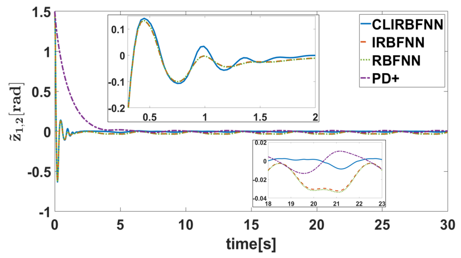
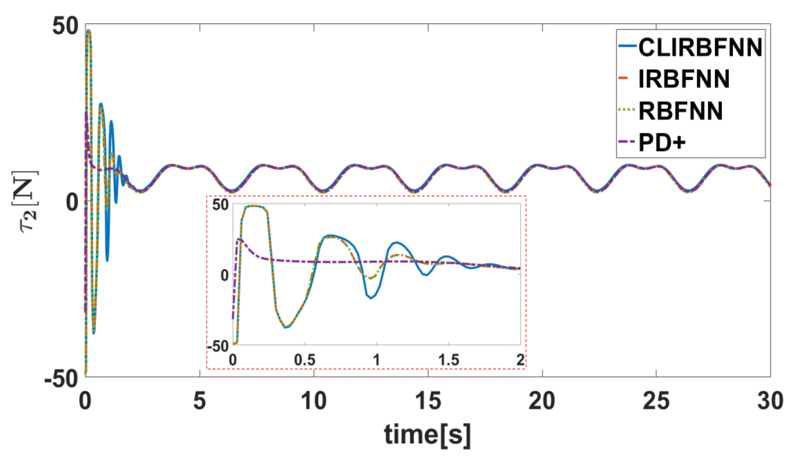
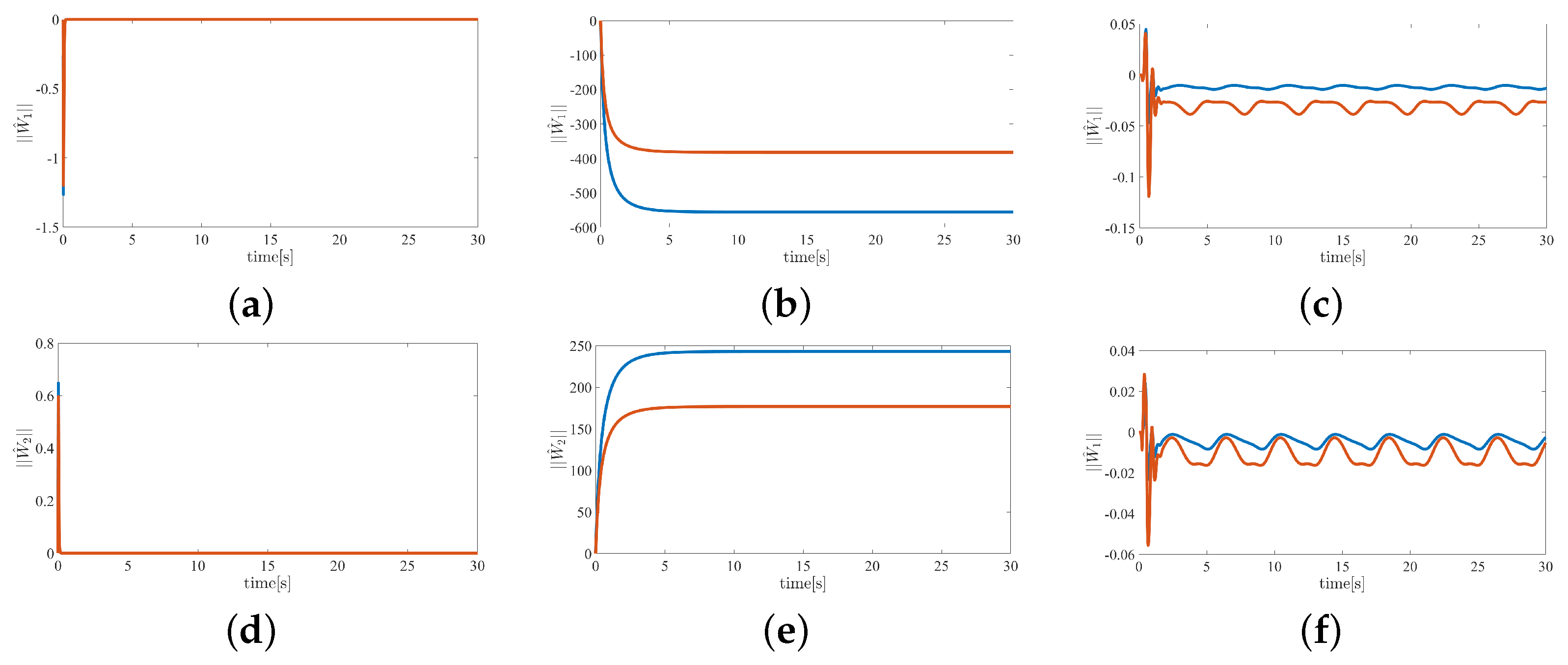
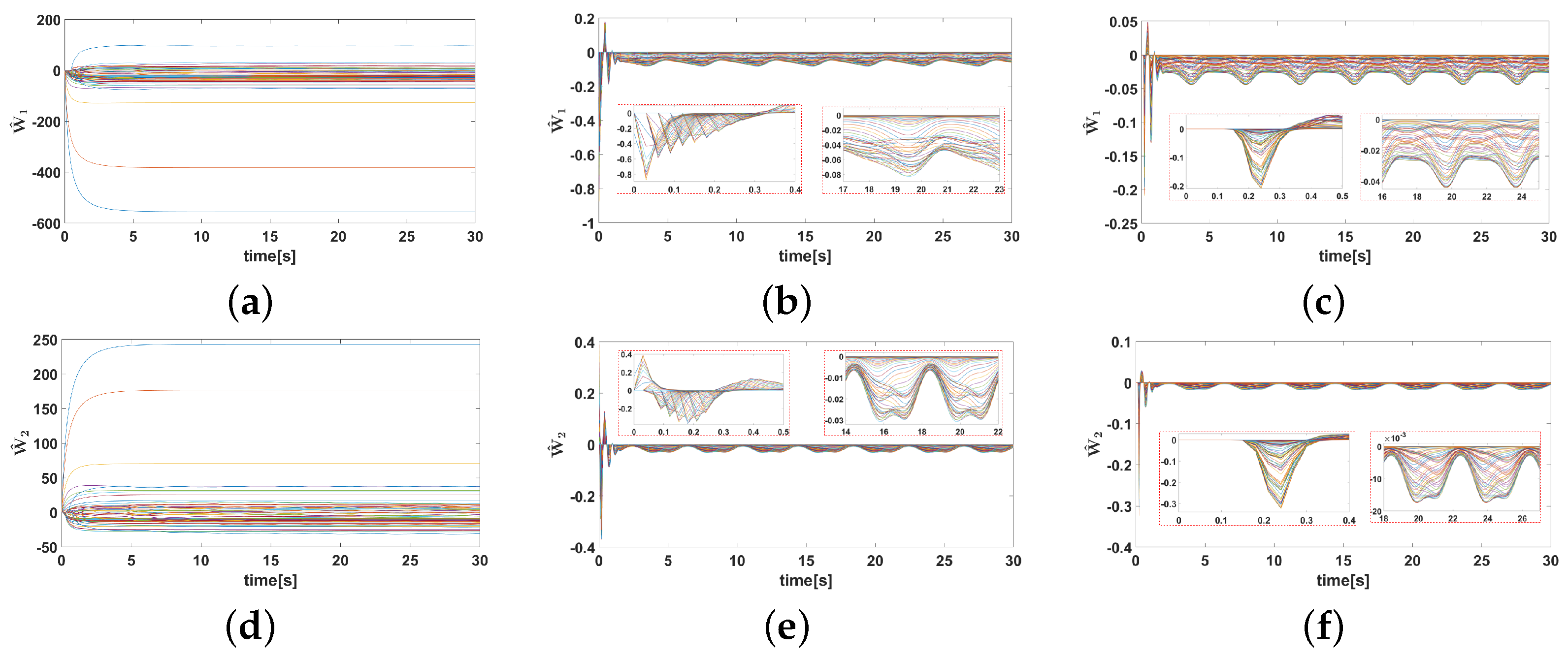
5. Simulation Verification

5.1. Simulation Settings

In order to verify the feasibility and effectiveness of the proposed control scheme, a simulation experiment was carried out on a two-DOF manipulator model [14], and the expression is shown in (53), while the model is shown in Figure 3. The meanings of the parameters in the expression are shown in

Table 1. The description of the 2-joint manipulator.

$H_{11}$	$(m_1+m_2)l_1^2+m_2{l}_2^2+2m_2{l}_1{l}_{2}cos{\theta }_2$
$H_{12}$	$m_2(l_2^2+l_1{l}_{2}cos{\theta }_2)$
$H_{21}$	$m_2(l_2^2+l_1{l}_{2}cos{\theta }_2)$
$H_{22}$	$m_2{l}_2^2$
$C_{11}$	$-m_2{l}_1{l}_2\dot{q_2}sin{\theta }_2$
$C_{12}$	$m_2{l}_1{l}_2(\dot{{\theta }_2}+\dot{{\theta }_1})sin{\theta }_2$
$C_{21}$	$m_2{l}_1{l}_2\dot{{\theta }_1}sin{\theta }_2$
$C_{22}$	0
$G_1$	$m_2{l}_{2}gcos({\theta }_1+{\theta }_2)+(m_1+m_2)l_{1}gcos{\theta }_1$
$G_2$	$m_2{l}_{2}gcos({\theta }_1+{\theta }_2)$

. The desired trajectory is shown in (54). The mass and length parameters of the linkage manipulator were set as follows $m_1=4$ kg, $m_2=2$ kg, $g=9.81$ N/kg, $l_1=0.5$ m, and $l_2=0.5$ m. The saturation torque of Joint 1 was selected as $100N$, and the saturation torque of Joint 2 was select as $50N$, i.e., $\overline{\tau }={[100,50]}^T$. The saturation characteristic parameter $\overline{u}$ is given as $\overline{u}={[300,300]}^T$.

$$\begin{array}{c}\hfill \left[\begin{array}{cc}{H}_{11}& H_{12}\\ H_{21}& H_{22}\end{array}\right]\left[\begin{array}{c}{\ddot{\theta }}_1\\ {\ddot{\theta }}_2\end{array}\right]+\left[\begin{array}{cc}{C}_{11}& C_{12}\\ C_{21}& C_{22}\end{array}\right]\left[\begin{array}{c}{\dot{\theta }}_1\\ {\dot{\theta }}_2\end{array}\right]+\left[\begin{array}{c}{G}_1\\ G_2\end{array}\right]=\left[\begin{array}{c}{\tau }_1\\ {\tau }_2\end{array}\right]\end{array}$$

(53)

$$\begin{array}{c}\hfill {\theta }_d\left(t\right)=\left[\begin{array}{c}{\theta }_{d1}\\ {\theta }_{d2}\end{array}\right]=\left[\begin{array}{c}-1+0.5\times sin\left(0.5\pi t\right)\\ 1+0.6\times cos\left(0.5\pi t\right)\end{array}\right]\end{array}$$

(54)

The parameters in the virtual controller and actual control law were chosen as $K_{12}=diag[3,2]$, $K_{13}=diag[4,2]$, $K_{22}=diag[3,2]$, and $K_{23}=diag[4,2]$. The relevant parameters of the INN are given as follows: $\sigma =0.5$, $\delta =0.9$. The maximum number of nodes in the network is 100, $\epsilon =0.5$. The parameters of the network weight update rate based on composite learning were chosen as $K_{32}=diag[4,4]$ and $K_{33}=diag[2,2]$. The fixed-time-related parameters were set to $\alpha =0.6$ and $\beta =2$.

In order to more intuitively compare the performance of the incremental neural network controller based on composite learning (CLIRBFNN), we set up a group of convincing comparative simulations. The comparative controllers adopted the fixed-time incremental neural network controller (IRBFNN), the general neural network controller (RBFNN), and the PD+ controller (PD+), and the weight update rate of the comparative controller adopted the traditional update rate, that is

$$\dot{\widehat{W}}={\Gamma }^{-1}(\Phi \left(x\right){\tilde{z}}_2-\lambda \widehat{W})$$

(55)

where $\Gamma =diag[2,2]$ and $\lambda =diag[10,10]$. The control law of the compared PD+ controller is

$$u=-K_p{\tilde{z}}_1-K_d{\dot{\tilde{z}}}_1+G$$

(56)

$${\tau }_i=\left\{\begin{array}{c}{\overline{\tau }}_{i}Sign\left(u_i\right),\left|u_i\right|>{\overline{\tau }}_i\hfill \\ u_i,\left|u_i\right|\le {\overline{\tau }}_i\hfill \end{array}\right.$$

(57)

where the gravity term G is fully compensated. The values of $K_p$ and $K_d$ were selected as $K_p=diag[100,40]$ and $k_d=diag[80,40]$.

In order to specifically compare the controllers under different initial states, three groups of different initial states were set, i.e., $\theta \left(0\right)=[-1,1]$, $\theta \left(0\right)=[-0.6,0.6]$, and $\theta \left(0\right)=[-0.5,0.5]$, and the corresponding initial position errors were ${\tilde{z}}_1\left(0\right)=[-2.6,2.6]$, ${\tilde{z}}_1\left(0\right)=[-1.5,1.5]$, and ${\tilde{z}}_1\left(0\right)=[-0.4,0.4]$. The purpose of this setting was to fully investigate the performance of the controller when the initial error is more than 20-times the preset steady-state error. On the other hand, the performance of the two joints under positive and negative errors can be observed. Moreover, the difference between the performance of the controller under a small initial error and a large initial error can be seen.

5.2. Result Analysis

The simulation results are presented in Figure 4, Figure 5, Figure 6, Figure 7, Figure 8, Figure 9, Figure 10, Figure 11 and Figure 12. Figure 4 and Figure 5 show the curves of the tracking error under different initial conditions. It can be seen that different initial values have a certain impact on the transient response, but have little impact on the steady-state error. This means that the designed fixed-time controller has good performance under different initial conditions. Figure 6, Figure 7, Figure 8 and Figure 9 present the tracking errors and control torques of Joint 1 and Joint 2 based on different controllers. It is obviously seen that the controller proposed in this paper can ensure that the error converges to a smaller neighborhood than the other compared controllers. Figure 10 shows the norm of the weight. We can see that the they are all bounded and can converge to constants. Figure 11 shows that each dimension weight value of the CLIRBFNN can eventually converge to the constant value, and adding new nodes to the network, the trained weights do not need to be retrained, which indicates that the CLIRBFNN adopted by the proposed controller has a high calculation efficiency. The weight update rate based on the IRBFNN and RBFNN was designed using Lyapunov stability, which was not applied to the error term of the network, so it can only be guaranteed to converge in a certain equilibrium interval. In terms of amplitude, the weight of the CLIRBFNN is at least three orders of magnitude higher than that of the IRBFNN and RBFNN, which expresses the effectiveness of composite learning in weight training. Figure 12 describes the network estimation error for Joint 1 and Joint 2 under the CLIRBFNN, IRBFNN, and RBFNN, respectively. For the CLIRBFNN, the network estimation error of each dimension will eventually converge to the smallest neighborhood near zero in a fixed time. For the IRBFNN and RBFNN, the network estimation error can only oscillate periodically in a large interval, and the oscillation period is positively related to the period of the desired trajectory.

In order to more quantitatively analyze the role of each control term in the control process, we analyzed the relative proportion of each control term. Blue refers to the first and second terms of $u_o$ in (39); red is the third term of $u_o$; green is the fourth term of $u_o$; yellow is the NN’s control term. Figure 12 depicts that, in the absence of composite learning control, i.e., the IRBFNN and RBFNN, the weights cannot be well trained, resulting in the proportion of network control terms being less than one-thousandth of the whole control process. Therefore, the approximation performance of the system is degraded, which is also the reason why the steady-state errors in Figure 6 and Figure 7 are larger than that of the proposed controller in this paper. From Figure 13a,d, it can be seen that, in the transient regulation stage, the proportion terms (blue) and fixed-time terms (red and green) account for a large proportion, which indicates that the transient regulation mainly depends on the non-network terms. In the process of steady-state regulation, the proportion of the CLIRBFNN terms exceeds $80\%$ of the total most of the time, and the proportion of the non-network control terms is very small, which shows that the CLIRBFNN compensates the uncertainty terms well and has excellent approximation performance.

Through the above analysis, the following conclusions can be drawn: the NN fixed-time controller based on composite learning can ensure that the network weights converge when the continuous excitation is not satisfied, and all error signals of the manipulator system can converge to a small neighborhood near zero in a fixed time with the input being saturated.

6. Conclusions

In this paper, a fixed-time adaptive tracking control scheme with actuator saturation was proposed for the manipulator system under the composite learning framework, combined with the INN control scheme. A new incremental neural network adaptive algorithm based on compound learning was designed, so that the estimation error information could be properly integrated into the adaptive law, which improved the estimation performance and relaxed the PE condition. At the same time, a hyperbolic tangent function was designed to solve the problem of asymmetric input saturation, and a backstepping recursive fixed-time control scheme was employed to design the controller. In addition, the stability analysis was carried out by using the fixed-time Lyapunov theory, which not only suppressed the input saturation, but also ensured the fixed-time convergence of all signals. Our future work will extend the presented scheme to a dual-arm robot and verify the proposed control approach by using the Baxter robot.

References

1. Li, Z.; Huang, B.; Ajoudani, A.; Yang, C.; Su, C.; Bicchi, A. Asymmetric bimanual control of dual-arm exoskeletons for human-cooperative manipulations. IEEE Trans. Robot. 2017, 34, 264–271. [Google Scholar] [CrossRef]
2. Li, R.; Qiao, H. A survey of methods and strategies for high-precision robotic grasping and assembly tasks—Some new trends. IEEE/ASME Trans. Mechatron. 2019, 24, 2718–2732. [Google Scholar] [CrossRef]
3. Zeng, C.; Yang, C.; Chen, Z. Bio-inspired robotic impedance adaptation for human-robot collaborative tasks. Sci. China Inf. Sci. 2020, 63, 170201. [Google Scholar] [CrossRef]
4. Lewis, F.L.; Liu, K.; Yesildirek, A. Neural net robot controller with guaranteed tracking performance. IEEE Trans. Neural Netw. 1995, 6, 703–715. [Google Scholar] [CrossRef] [PubMed]
5. Chen, Z.; Liu, Y.; He, W.; Qiao, H.; Ji, H. Adaptive-neural-network-based trajectory tracking control for a nonholonomic wheeled mobile robot with velocity constraints. IEEE Trans. Ind. Electron. 2020, 68, 5057–5067. [Google Scholar] [CrossRef]
6. Yang, C.; Chen, C.; He, W.; Cui, R.; Li, Z. Robot learning system based on adaptive neural control and dynamic movement primitives. IEEE Trans. Neural Netw. Learn. Syst. 2018, 30, 777–787. [Google Scholar] [CrossRef]
7. Zhao, K.; Song, Y. Neuroadaptive robotic control under time-varying asymmetric motion constraints: A feasibility-condition-free approach. IEEE Trans. Cybern. 2018, 50, 15–24. [Google Scholar] [CrossRef]
8. Ma, Z.; Huang, P.; Kuang, Z. Fuzzy approximate learning-based sliding mode control for deploying tethered space robot. IEEE Trans. Fuzzy Syst. 2020, 29, 2739–2749. [Google Scholar] [CrossRef]
9. Su, H.; Qi, W.; Chen, J.; Zhang, D. Fuzzy Approximation-based Task-Space Control of Robot Manipulators with Remote Center of Motion Constraint. IEEE Trans. Fuzzy Syst. 2022, 30, 1564–1573. [Google Scholar] [CrossRef]
10. Yang, C.; Jiang, Y.; Na, J.; Li, Z.; Cheng, L.; Su, C. Finite-time convergence adaptive fuzzy control for dual-arm robot with unknown kinematics and dynamics. IEEE Trans. Fuzzy Syst. 2018, 27, 574–588. [Google Scholar] [CrossRef]
11. Huang, H.; Zhang, T.; Yang, C.; Chen, C.P. Motor learning and generalization using broad learning adaptive neural control. IEEE Trans. Ind. Electron. 2019, 67, 8608–8617. [Google Scholar] [CrossRef]
12. Miao, Z.; Liu, Y.; Wang, Y.; Chen, H.; Zhong, H.; Fierro, R. Consensus with persistently exciting couplings and its application to vision-based estimation. IEEE Trans. Cybern. 2019, 51, 2801–2812. [Google Scholar] [CrossRef]
13. Wang, C.; Hill, D.J. Learning from neural control. IEEE Trans. Neural Netw. 2006, 17, 130–146. [Google Scholar] [CrossRef]
14. Yang, C.; Teng, T.; Xu, B.; Li, Z.; Na, J.; Su, C. Global adaptive tracking control of robot manipulators using neural networks with finite-time learning convergence. Int. J. Control Autom. Syst. 2017, 15, 1916–1924. [Google Scholar] [CrossRef]
15. Wang, C.; Wang, M.; Liu, T.; Hill, D.J. Learning from ISS-modular adaptive NN control of nonlinear strict-feedback systems. IEEE Trans. Neural Netw. Learn. Syst. 2012, 23, 1539–1550. [Google Scholar] [CrossRef]
16. Pan, Y.; Sun, T.; Liu, Y.; Yu, H. Composite learning from adaptive backstepping neural network control. Neural Netw. 2017, 95, 134–142. [Google Scholar] [CrossRef]
17. Guo, K.; Pan, Y.; Yu, H. Composite learning robot control with friction compensation: A neural network-based approach. IEEE Trans. Ind. Electron. 2018, 66, 7841–7851. [Google Scholar] [CrossRef]
18. Chen, M.; Ge, S.S.; Ren, B. Adaptive tracking control of uncertain MIMO nonlinear systems with input constraints. Automatica 2011, 47, 452–465. [Google Scholar] [CrossRef]
19. Bai, W.; Zhou, Q.; Li, T.; Li, H. Adaptive reinforcement learning neural network control for uncertain nonlinear system with input saturation. IEEE Trans. Cybern. 2019, 50, 3433–3443. [Google Scholar] [CrossRef]
20. Wen, C.; Zhou, J.; Liu, Z.; Su, H. Robust adaptive control of uncertain nonlinear systems in the presence of input saturation and external disturbance. IEEE Trans. Autom. Control 2011, 56, 1672–1678. [Google Scholar] [CrossRef]
21. Zhou, Q.; Wang, L.; Wu, C.; Li, H.; Du, H. Adaptive fuzzy control for nonstrict-feedback systems with input saturation and output constraint. IEEE Trans. Syst. Man Cybern. Syst. 2016, 47, 1–12. [Google Scholar] [CrossRef]
22. He, W.; Dong, Y.; Sun, C. Adaptive neural impedance control of a robotic manipulator with input saturation. IEEE Trans. Syst. Man Cybern. Syst. 2015, 46, 334–344. [Google Scholar] [CrossRef]
23. Du, J.; Hu, X.; Krstić, M.; Sun, Y. Robust dynamic positioning of ships with disturbances under input saturation. Automatica 2016, 73, 207–214. [Google Scholar] [CrossRef]
24. Li, Y.; Wang, T.; Liu, W.; Tong, S. Neural network adaptive output-feedback optimal control for active suspension systems. IEEE Trans. Syst. Man Cybern. Syst. 2022, 52, 4021–4032. [Google Scholar] [CrossRef]
25. Bhat, S.P.; Bernstein, D.S. Finite-time stability of continuous autonomous systems. SIAM J. Control Optim. 2000, 38, 751–766. [Google Scholar] [CrossRef]
26. Cui, B.; Xia, Y.; Liu, K.; Shen, G. Finite-time tracking control for a class of uncertain strict-feedback nonlinear systems with state constraints: A smooth control approach. IEEE Trans. Neural Netw. Learn. Syst. 2020, 31, 4920–4932. [Google Scholar] [CrossRef]
27. Wang, F.; Chen, B.; Lin, C.; Zhang, J.; Meng, X. Adaptive neural network finite-time output feedback control of quantized nonlinear systems. IEEE Trans. Cybern. 2017, 48, 1839–1848. [Google Scholar] [CrossRef]
28. Fan, Y.; Li, Y.; Tong, S. Adaptive finite-time fault-tolerant control for interconnected nonlinear systems. Int. J. Robust Nonlinear Control 2021, 31, 1564–1581. [Google Scholar] [CrossRef]
29. Lv, M.; Li, Y.; Pan, W.; Baldi, S. Finite-time fuzzy adaptive constrained tracking control for hypersonic flight vehicles with singularity-free switching. IEEE/ASME Trans. Mechatron. 2022, 27, 1594–1605. [Google Scholar] [CrossRef]
30. Polyakov, A. Nonlinear feedback design for fixed-time stabilization of linear control systems. IEEE Trans. Autom. Control 2011, 57, 2106–2110. [Google Scholar] [CrossRef] [Green Version]
31. Jin, X. Adaptive fixed-time control for MIMO nonlinear systems with asymmetric output constraints using universal barrier functions. IEEE Trans. Autom. Control 2018, 64, 3046–3053. [Google Scholar] [CrossRef]
32. Zhang, Y.; Wang, F. Observer-based fixed-time neural control for a class of nonlinear systems. IEEE Trans. Neural Netw. Learn. Syst. 2021, 33, 2892–2902. [Google Scholar] [CrossRef]
33. Huang, C.; Liu, Z.; Chen, C.P.; Zhang, Y. Adaptive Fixed-Time Neural Control for Uncertain Nonlinear Multiagent Systems. IEEE Trans. Neural Netw. Learn. Syst. 2022. early access. [Google Scholar] [CrossRef]
34. He, W.; Kang, F.; Kong, L.; Feng, Y.; Cheng, G.; Sun, C. Vibration Control of a Constrained Two-Link Flexible Robotic Manipulator With Fixed-Time Convergence. IEEE Trans. Cybern. 2021, 52, 5973–5983. [Google Scholar] [CrossRef]
35. Huang, H.; Lu, Z.; Wang, N.; Yang, C. Fixed-time Adaptive Neural Control for Robot Manipulators with Input Saturation and Disturbance. In Proceedings of the 2022 27th International Conference on Automation and Computing (ICAC), Bristol, UK, 1–3 September 2022; p. 22136904. [Google Scholar]
Figure 1. The schematic diagram of the incremental neural network.
Actuators 11 00373 g001
Figure 2. The overview of the proposed control scheme.
Actuators 11 00373 g002
Figure 3. The model of the 2-DOF manipulator.
Actuators 11 00373 g003
Figure 4. Error z ˜ 1 , 1 with different initial values.
Actuators 11 00373 g004
Figure 5. Error z ˜ 1 , 2 with different initial values.
Actuators 11 00373 g005
Figure 6. The tracking error of Joint 1.
Actuators 11 00373 g006
Figure 7. The tracking error of Joint 2.
Actuators 11 00373 g007
Figure 8. The torque of Joint 1.
Actuators 11 00373 g008
Figure 9. The torque of Joint 2.
Actuators 11 00373 g009
Figure 10. The norm of the weights for the two joints based on the CLIRBFNN, IRBFNN, and RBFNN. (ac) show the norm of the weights for Joint 1. (df) show the norm of the weights for Joint 2.
Actuators 11 00373 g010
Figure 11. The weight of two joints based on the CLIRBFNN, IRBFNN, and RBFNN. (ac) show the weights of Joint 1. (df) show the weights of Joint 2.
Actuators 11 00373 g011
Figure 12. The estimation error based on the CLIRBFNN, IRBFNN, and RBFNN. (ac) show the estimation error of Joint 1. (df) show the estimation error of Joint 2.
Actuators 11 00373 g012
Figure 13. The torque ratio law under different NN control. (ac) show the proportion of Joint 1. (df) show the proportion of Joint 2.
Actuators 11 00373 g013