Dynamic Control of a Novel Planar Cable-Driven Parallel Robot with a Large Wrench Feasible Workspace

Abstract

Cable-Driven Parallel Robots (CDPRs) are special manipulators where rigid links are replaced with cables. The use of cables offers several advantages over the conventional rigid manipulators, one of the most interesting being their ability to cover large workspaces since cables are easily winded. However, this workspace coverage has its limitations due to the maximum permissible cable tensions, i.e., tension limitations cause a decrease in the Wrench Feasible Workspace (WFW) of these robots. To solve this issue, a novel design based in the addition of passive carriages to the robot frame of three degrees-of-freedom (3DOF) fully-constrained CDPRs is used. The novelty of the design allows reducing the variation in the cable directions and forces increasing the robot WFW; nevertheless, it presents a low stiffness along the x direction. This paper presents the dynamic model of the novel proposal together with a new dynamic control technique, which rejects the vibrations caused by the stiffness loss while ensuring an accurate trajectory tracking. The simulation results show that the controlled system presents a larger WFW than the conventional scheme of the CDPR, maintaining a good performance in the trajectory tracking of the end-effector. The novel proposal presented here can be applied in multiple planar applications.

1. Introduction

Parallel manipulators are a type of robot in which the end-effector is controlled by and connected to driving rigid links, called limbs. These robots are designed for achieving high stiffness and high payload capacity at the end-effector [1]; therefore, the weight of the links and their maximum strokes may considerably limit the velocities and the feasible workspace.

In order to overcome these evident limitations, cable-driven parallel robots have been introduced in the last two decades. In these systems, lightweight flexible cables actuate the end-effector. Each cable is wound around a winch, which is driven by an actuator. The winch can provide from millimetres up to several metres of cable, not only enabling large workspaces, but also assuring rather limited inertia, if compared to the rigid links’ counterparts, and high velocities at the end-effector. CDPRs also provide the possibility of implementing deployable and reconfigurable topologies, which may expand the application of robotics in new environments, e.g., search and rescue operations [2,3], motion aiding systems [4,5], large buildings’ maintenance and construction [2], entertainment [6], manufacturing or heavy handling [7], and service [8], but also considering classical high-speed pick and place manipulators in [9,10]. Applications related to the large working volume are the NIST Robocrane [11] and the five-hundred-metre Aperture Spherical Telescope (FAST), as reported in [12].

Despite these advantages, the current development of CDPRs seems to be limited mainly by the consequences deriving from the unilateral nature of cables; they can only pull the end-effector, but not push it. For operating a CDPR, the cable tensions must be kept positive, e.g., tensed during motion. If a cable or more cables become slack, the end-effector cannot be controlled properly for following a prescribed trajectory or exert the required wrench to perform a given task. This occurrence may introduce relevant performance and safety issues, since the control of the end-effector may be lost [13]. Nevertheless, the use of CDPRs seems very promising and has already been suggested in several different operation fields, such as heavy handling and industrial manufacturing, but also medical rehabilitation, home assistance, or sport shooting.

In the future, a wide use of CDPRs is expected thanks to their lightweight structure, which makes them energy efficient, modularity and reconfigurability, which makes them flexible and easy to transport, and finally, the potentially high dynamics and payload capacity, which makes them effective in a wide range of industrial applications.

In the analysis and design of CDPRs, but also for the operating issues and control, it is of great importance considering the number of active cables and their collocations; therefore overconstrained CDPRs have been defined as robots having a number of actuated cables higher than the EE degrees-of-freedom (DoFs) so that the cables can pull each other. Underconstrained CDPRs are those for which the cables cannot control all the DOFs of the robot; usually, under this category, the cable suspended robots fall; they are defined as CDPRs for which all active cables are suspending the EE, and the bottom of the robot is free from cables [14,15]. In [16], a point-to-point trajectory model was proposed for suspended CDPRs.

A large amount of research on CDPRs was initially devoted to workspace determination by referring to the so-called wrench closure workspace (WS) [17], i.e., a pose belongs to the WS if the static equilibrium is satisfied by positive tensions or tensions bounded by given limits of wrench feasible WS [18]. Therefore, limits were defined as the highest load capacity for the upper bound and cables’ slackness avoidance, for the lower bounds, modelling an ideal cable, neglecting mass and elasticity.

Advanced models for the kinetostatic analysis consider the mass and elasticity of the cables to take into account sag effects in positioning capabilities [19,20,21,22]. In particular, direct and inverse kinematic models have been proposed.

Nevertheless, taking into account many practical applications, such as those mentioned above, a static or quasi-static assumption is rather limited since dynamic conditions are involved. In particular, vibrations are not simply induced by rapid end-effector velocity changes, wind disturbance, and/or friction of the cables around pulleys [23]. In applications requiring high performances, especially dynamic performances, e.g., [9,24], or in the presence of wind, e.g., [25,26], vibrations are an issue since they can affect the positioning accuracy of the end-effector and yield fluctuations around a desired nominal end-effector trajectory.

Dynamic models of CDPRs were initially developed neglecting the contribution of the cables, i.e., the cables were assumed as mass-less and non-elastic elements, as reported in [27]. Natural frequency is widely used in the literature as an index for the dynamic stiffness evaluation of CDPRs [23,28]. Several works proposing the stiffness analysis of CDPRs have been introduced by considering cable elasticity, but negligible cable mass [29]. In [30,31], cables were modelled as mass-less elastic springs and additionally taut strings, for analysing the contribution of the cables’ flexibility in the axial and transverse directions to the vibrations of the moving mass constituting the end-effector. The kinematics and dynamics of the IPAnema3 cable robot were proposed in [32] by modelling cables as spring–damper elements with variable spring and damping rates due to the change in effective lengths. The above-mentioned model presents limitations, especially in the case of CDPRs with heavy and/or long-span cables. In fact, the axial cable stiffness is not the only source of the static stiffness. Sag-introduced stiffness should also be considered. As actual trends, research on CDPRs is focusing on the dynamic stiffness for its importance to have better stability, positioning accuracy, and flexibility [33]. The stiffness of a vibrating cable depends on the mechanical properties, the configuration of the cables, environmental effects, the initial cable tension, and cable motion [34].

Most of the reported works in the literature consider both cable elasticity and cable mass in two-dimensional inclined cables for dynamic analyses of the CDPRs with free vibration [34,35], i.e., without external forces acting on the system. However, for some applications, the forced vibrations are the result of external excitements/disturbances.

The vibration analysis for CDPRs with a large workspace was proposed in [36,37], where the cables were modelled with distributed mass and axial stiffness. The resulting solving equations were solved using different numerical techniques, e.g., converting to ordinary differential equations using the finite element method [36] and the assumed-mode method [37].

This paper presents a novel planar CDPR design based on adding passive carriages to the frame, providing the ability to passively reconfigure the distal anchor points of the robot [38]. The mechanical scheme together with the workspace gain and another kinematics issued were presented in [39].

Some works present active reconfigurable cable-driven parallel robots (RCDPRs) (e.g., [40]) or variable-structure cable-driven parallel robots (VSCR) (e.g., [41]. In RCDPRs, the position of the distal anchor points can be controlled by actuators, since in VSCRs, the distal anchor points are relocated by adding circumventing obstacles. In this sense, the scheme of this work pretends to increase the feasible workspace of the robot without adding more actuators.

The previous work [39] concluded that the addition of a passive carriage notoriously increases the feasible workspace of the robot, but on the contrary, the end-effector suffers a loss of stiffness along the horizontal axis, and non-desirable vibrations appear on the end-effector during its manoeuvres.

This work continues the work in [39]. The objective is to develop a dynamic control that allows the end-effector positioning

For this purpose, this paper is focused on the following:

(a)

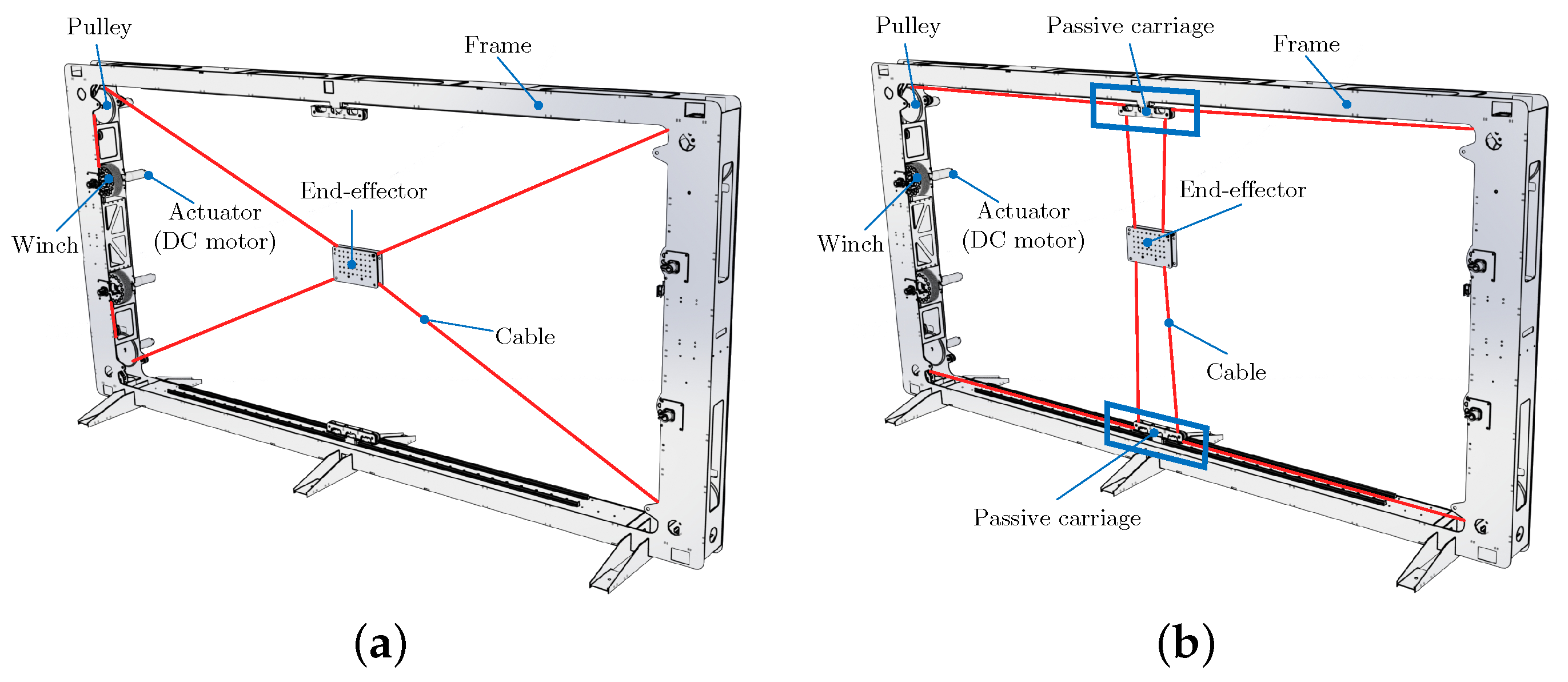
To present the dynamics model of the robot, which includes the dynamics model of the passive carriages. The addition of these carriages makes the system have five degrees-of-freedom and four actuators (underconstrained), but only three of them shall be controlled (fully constrained).

(b)

To develop a suitable trajectory generator. In this sense, the distal anchor points [38] of the robot are passively reconfigurable, and trajectory planning for the underconstrained scheme shall be applied. Our proposal is based the trajectory generator on the statically feasible workspace [42].

(c)

To implement a dynamic control that tackles the problems of positive tension and vibrations’ rejection, owing to the low stiffness that the robot presents in the horizontal axis. In this sense, a novel control approach based on the addition of a control signal offset together with conventional PID controllers are also presented.

At the end, our final objective is to obtain a planar CDPR with a large workspace with an accurate end-effector position control.

This paper is organised as follows: Section 2 describes the novel proposal and presents the nomenclature. Section 3 details the mathematical model of the robot, including the dynamics model, required to design a proper control approach, which is presented in Section 4. Section 5 and Section 6, respectively, show the simulation and experimental results, and finally, Section 6 discusses these results and summaries the main conclusions.

2. System Description

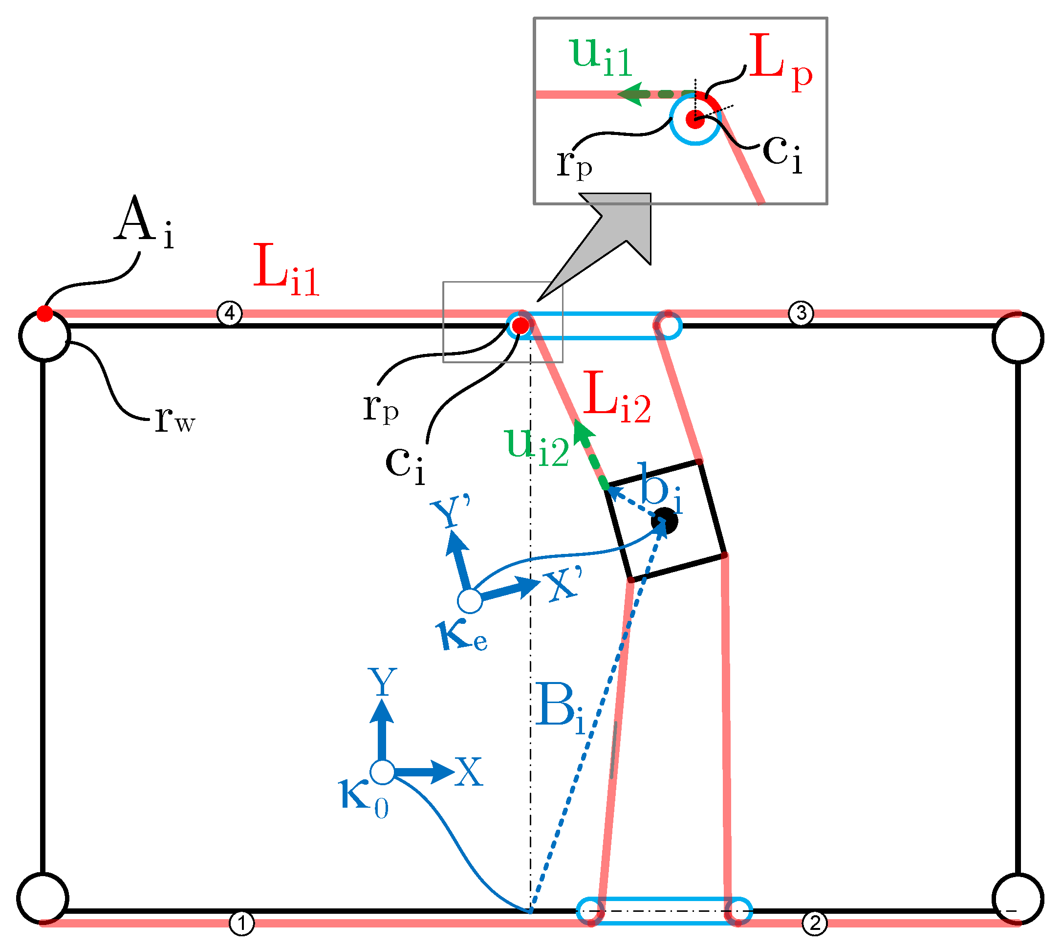
2.1. Overall Description

This paper is focused on a planar fully constrained CDPR [38]. The end-effector has three degrees-of-freedom, and its pose is commanded by four cables. At the same time, each cable is driven by a motor (placed at the frame) that rolls in or out the cable into/from a winch. A scheme of this conventional planar CDPR is shown in Figure 1a.

Figure 1. Scheme comparison. (a) Conventional scheme; (b) new proposal.

Our proposal is based on the addition of passive carriages over the conventional scheme. The end-effector has the same three degrees-of-freedom, and the motors drive the length of the four cables in the same way as in the conventional scheme. Nevertheless, now, each cables is led to a pulley placed in a carriage that can freely move over a linear guide. Note that Cables 1–2 and 3–4 are attached to the lower and upper carriages, respectively. The scheme of the proposal is shown in Figure 1b. Our previous work [39] presented the proposal, reporting the workspace gain in comparison to the conventional scheme as the main advantage.

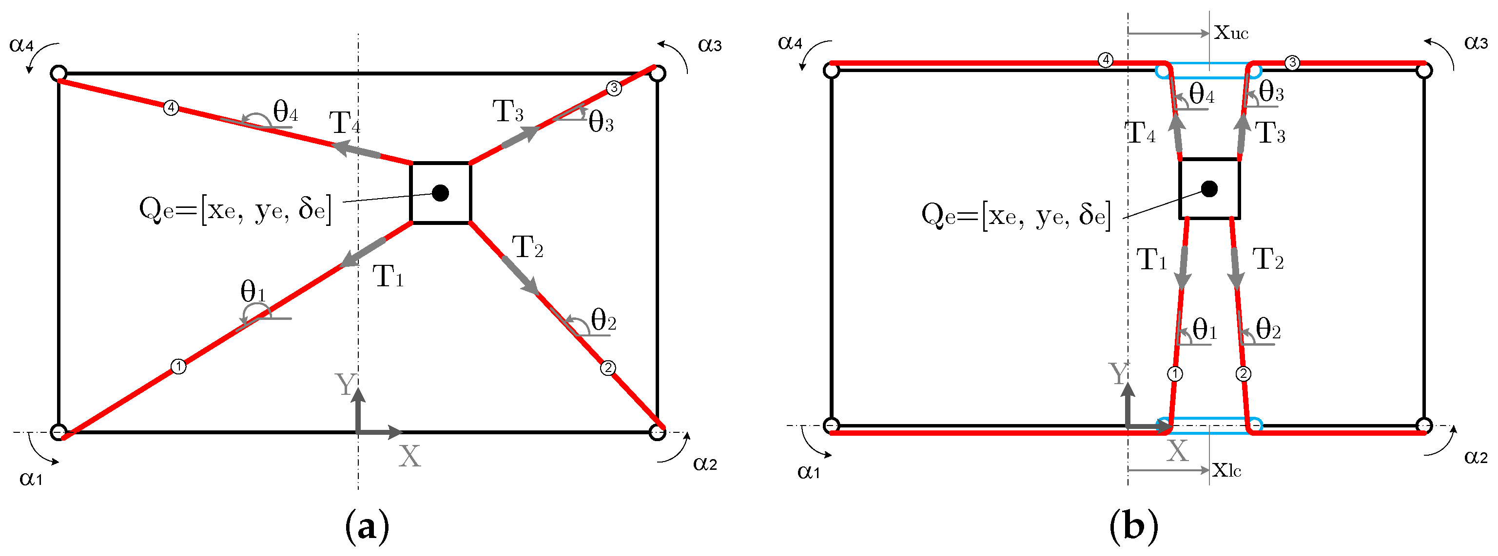
2.2. Nomenclature

In a preliminary way, Figure 2 shows the basic nomenclature, where for both schemes:

Figure 2. Scheme for nomenclature. (a) Conventional scheme; (b) new proposal.

• The end-effector pose is defined as $\mathbf{Q}$${}_e$ $=[x_e,y_e,{\delta }_e]$.
• The tension of the cables is $T_i$ for $i=1$ to 4.
• The angle of the cables is ${\theta }_i$ for $i=1$ to 4.
• The angle of the motors is defined as ${\alpha }_i$ for $i=1$ to 4.

Finally, for the novel proposal, the horizontal coordinate of the upper carriage is denote as $x_{uc}$ and for the lower carriage as $x_{lc}$

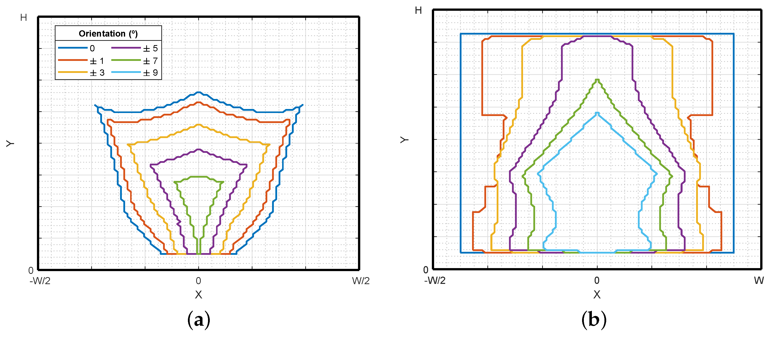
2.3. Workspace and Stiffness Comparison

Assume that both schemes are in the vertical plane and gravity has an influence on the Y axis force equilibrium. Under a static point of view, the workspace can be easily obtained by establishing an end-effector pose and checking if a tension combination $T={[T_1,T_2,T_3,T_4]}^T$ exists that allows a force/torque equilibrium at the end-effector (for the conventional scheme) and at the end-effector and both carriages (for the novel scheme). This tension combination must remain inside of the allowed limit $[T_{min},T_{max}]$ as any CDPR (see [38] for more details).

The equilibrium equations for the conventional scheme can be written as:

$${\mathbf{A}}_{\mathbf{s}}({\mathbf{Q}}_e,x_{uc},x_{lc})\mathbf{T}+{\mathbf{W}}_e=0$$

(1)

where ${\mathbf{A}}_{\mathbf{s}}$ is a geometrical matrix that depends on the parameters of the robot and the end-effector pose (e.g., [38]) and $\mathbf{W}$${}_e={[0,-m_e·g,0]}^T$ is the external force array, with $m_e$ the end-effector mass and g the gravity acceleration. Only for illustrative purposes, for several end-effector orientations (${\delta }_e=0^{\circ }$, $\pm 1^{\circ }$, $\pm 3^{\circ }$, $\pm 5^{\circ }$, $\pm 7^{\circ }$, and $\pm 9^{\circ }$), the feasible workspace, defined as the set of points that fulfil (1), is represented for both schemes, conventional and the new proposal, in Figure 3, where W and H are the width and the height of the frame, respectively. These results are detailed in [39].

Figure 3. Workspace comparison. (a) Conventional scheme; (b) new proposal.

This workspace gain makes the proposal suitable to apply planar CDPRs, which require a complete workspace with regard to the frame size. Nevertheless, on the contrary, the proposed scheme presents lower stiffness along the horizontal axis, which yields a non-desirable vibration during the robot manoeuvres. The stiffness matrix of a CDPR, defined by Pott [43], is the sum of the cable and the geometric stiffness matrices. The cable stiffness matrix depends on the cables’ stiffness and the robot structure matrix $\mathbf{A}$${}_e^T$ (further discuss), which in turn depends on the robot geometry and end-effector’s/carriages’ position. Furthermore, the geometric stiffness matrix depends on the cable force distribution and the $\mathbf{A}$${}_e^T$ variation with end-effector pose. In order to evaluate how the novel design is affected, the directional stiffness index defined by Moradi [44] is used. Employing the parameters from Table 1, we are able to compare the stiffness of the new CDPR with that of a conventional design. For illustrative purposes, the robot frame is swept on equally spaced points to determine the end-effector non-oriented position. Applying the method proposed by Pott in [45], the force distribution is obtained within the cable force limits of $[10,100]$ N. Figure 4 compares the stiffness map obtained under a force applied in the x axis positive direction for both schemes. A significant decrease of the stiffness can be observed when applying forces in the x axis. More explanation about these results can be found in [39].

Table 1. Model parameters.

Subsystem	Parameter	Value
Frame	H	$0.8$ m
	W	$1.2$ m
Carriages	$w_{cl}$	$0.2$ m
	$w_{cu}$	$0.2$ m
	$m_c$	3 kg
	$b_c$	$0.2$ Ns/m
Motor/winch set	J	4.61 × ${10}^{-4}$ Kgm${}^2$
	$b_m$	$7.69\times {10}^{-3}$ Nms
	r	$0.04$ m
End-effector	$m_e$	1 kg
	w	$0.1$ m
	h	$0.1$ m
	$I_e$	$2\times {10}^{-3}$ Kgm${}^2$
Controllers	${\omega }_c$	40 rad/s
	${\phi }_m$	${60}^{\circ }$
	$K_p$	$0.6357$
	$K_d$	$0.0121$
	$K_i$	$0.55$

Figure 4. X axis stiffness comparison. (a) Conventional scheme; (b) new proposal.

As a conclusion, the proposal here presents a much larger feasible workspace with regard to the conventional scheme, but, on the other hand, the horizontal stiffness is much lower, producing non-desirable vibration during the robot movements.

In this sense, the next section introduces the mathematical model of the system, including the dynamic model, in order to design a control approach that allows rejecting the negative effects of the low horizontal stiffness of the proposal.

3. Mathematical Model

3.1. Kinematic Model

In this section, the inverse kinematic model is presented. This model will be used to implement the dynamics model and in the control approach of the robot. The inverse kinematic determines the actuator position, ${\alpha }_1$ to ${\alpha }_4$, to obtain a desired end-effector pose ${\mathbf{Q}}_e$ $={[x_e,y_e,{\delta }_e]}^T$.

First of all, to complete the nomenclature of Section 2.2, it is required to define some still missing geometrical parameters of the robot: end-effector width, (w), end-effector height (h), upper carriage width ($w_{uc}$), and lower carriage width ($w_{lc}$).

It must be pointed out that the geometry model was obtained by taking into account the passive pulley radius effect on the cable lengths [38]. The carriages’ widths, $w_{cu},w_{cl}$, are considered to be the distance between the passive pulleys’ centres; the cable goes vertically from the pulley centre to the winch, although the contact point in the pulley from the end-effector depends on the positioning between the carriage and the end-effector.

The frame is defined by the proximal anchor points (PAPs), $A_i\in R^2(i=1,\dots ,4)$, with respect to the World reference system ${\kappa }_0$ shown in Figure 5. On the other hand, the end-effector geometry is defined by the distal anchor points (DAPs), $b_i\in R^2(i=1,\dots ,4)$, in the local reference system ${\kappa }_e$ with respect to the end-effector. Figure 5 is included to clarify all vectors used in the kinematics model and the points of interest.

Figure 5. Nomenclature: arrays and points of interest.

The end-effector pose, ${\mathbf{Q}}_e={[x_e,y_e,{\delta }_e]}^T$, is a combination between its position, ${\mathbf{q}}_e={[x_e,y_e]}^T$, and orientation, ${\delta }_e$. In this sense, the DAP with respect to ${\kappa }_0$ can be obtained as

$${\mathbf{B}}_i={\mathbf{q}}_e+{\mathbf{R}}_z\left({\delta }_e\right)·{\mathbf{b}}_i,$$

(2)

where

$${\mathbf{R}}_z\left(\delta \right)=\left[\begin{array}{ccc}cos\left(\delta \right)& & -sin\left(\delta \right)\\ sin\left(\delta \right)& & cos\left(\delta \right)\end{array}\right]$$

(3)

is the rotation matrix around the z axis. The position of the passive carriages with respect to ${\kappa }_0$ is defined as $x_{uc}$ and $x_{lc}$ for the upper and lower carriage. Taking this into account, the position of the passive pulley centres with respect to ${\kappa }_0$ is defined as

$$c_i=x_c+v_{ci},$$

(4)

with $x_c=x_{lc}$ for $i=1,2$, $x_c=x_{uc}$ for $i=3,4$ and $v_{ci}$ being the vector that goes from the carriage centre to the ith passive pulley centre.

As is known from earlier, parallel robots have two possible kinematic formulations. The inverse kinematic model obtains the cable lengths, $\mathbf{L}={[L_1,\dots ,L_4]}^T$, from an arbitrary end-effector pose:

$$\mathbf{L}={\mathbf{\phi }}^{IK}({\mathbf{Q}}_e,x_{lc},x_{uc})$$

(5)

The cables are considered massless, so that they are formulated as straight lines connecting the previously defined geometric points. Considering the scheme in Figure 5 and the effect of the passive pulleys’ radius, $r_p$, the total cable length yields $L_i=L_{i,1}+L_p+L_{i,2}$, with:

$$\begin{array}{c}{L}_{i,1}=|A_{i,x}-c_{i,x}|\\ L_{i,2}=\sqrt{B{C}_i^2-r_p^2}\\ L_p={\beta }_u{r}_p,\end{array}$$

(6)

where $B{C}_i=\left|\right|B_i-c_i\left|\right|$, $\left|\right|·\left|\right|$ being the two-norm of the vector · and ${\beta }_u$ the angle formed by the cable rolled in the passive carriage pulleys, which can be obtained by means of $c_i$ and $B_i$ as:

$${\beta }_u={cos}^{-1}\left(\frac{L_{i,2}}{B{C}_i}\right)+{cos}^{-1}\left(\frac{\mathrm{sign}(c_{i,x}-A_{i,x}{d}_x)}{B{C}_i}\right),$$

(7)

$d_x=B_{i,x}-c_{i,x}$, $\mathrm{sign}\left(x\right)$ being the sign function. The actuators angle for an arbitrary end-effector and carriages’ pose can be obtained by:

$$\mathbf{\alpha }=\frac{\mathbf{L}-L_0}{r_w},$$

(8)

where $\mathbf{\alpha }={[{\alpha }_1,\dots ,{\alpha }_4]}^T$ is the array of the joint coordinates, $L_0$ is the initial cable lengths defined for an initial end-effector and carriages’ pose/position, ${\mathbf{Q}}_{e0},x_{lc0},x_{uc0}$, and $r_w$ is the combined winch radius taking into account any gearbox connected to the actuators.

On the contrary, the forward kinematic consists of determining the end-effector pose, ${\mathbf{Q}}_e$, for a given set of joint coordinates, $\mathbf{\alpha }$:

$${\mathbf{Q}}_e={\mathbf{\phi }}^{FK}(\mathbf{\alpha },x_{lc},x_{uc})$$

(9)

Due to its much more complicated development and owning to the fact that the forward kinematics has infinite solutions [38], only the inverse kinematics is fully developed and applied for the control scheme.

The inverse kinematic model developed here is used to implement the dynamic model presented in the following section and for the control scheme detailed in Section 4.

3.2. Dynamic Model

While the kinematics and static models relate the end-effector and carriage positions to the cable lengths and tensions, the dynamics of the system describes its behaviour. The input variables to the system are the torque exerted by the motors, ${\tau }_i$ with $i=1,\dots ,4$, and the output is the end-effector pose, ${\mathbf{Q}}_e={[x_e,y_e,{\delta }_e]}^T$.

Due to the novel design, the dynamics of the motor sets, end-effector, and carriages must be considered to develop a representative model. The motor and end-effector dynamics is equal to the one used for a conventional CDPR design. The end-effector dynamics is represented by the following expression:

$${\mathbf{M}}_e{\ddot{\mathbf{Q}}}_e={\mathbf{A}}_e^T({\mathbf{Q}}_e,x_{lc},x_{uc})\mathbf{T}+{\mathbf{W}}_e,$$

(10)

where

$${\mathbf{M}}_e=\left[\begin{array}{ccc}{m}_e& 0& 0\\ 0& m_e& 0\\ 0& 0& I_e\end{array}\right],$$

(11)

$m_e$ being the end-effector mass, $I_e$ the end-effector rotational inertia, $\mathbf{T}={[T_1,\cdots ,T_4]}^T$ the cable tensions’ vector, ${\mathbf{W}}_e={[0,-m_{e}g,0]}^T$ the external wrench vector, which is only subjected to its own weight, and ${\mathbf{A}}_e^T$ the structure matrix, which yields:

$${\mathbf{A}}_e^T=\left[\begin{array}{ccccc}{\mathbf{u}}_{12}& & \cdots & & {\mathbf{u}}_{m2}\\ {\mathbf{R}}_z\left({\delta }_z\right){\mathbf{b}}_1\times {\mathbf{u}}_{12}& & \cdots & & {\mathbf{R}}_z\left({\delta }_z\right){\mathbf{b}}_m\times {\mathbf{u}}_{m2}\end{array}\right],$$

(12)

${\mathbf{u}}_{i,2}={\mathbf{R}}_z\left({\beta }_u\right){\mathbf{e}}_x$ being the unity vector containing the directions in which the cable forces are exerted on the end-effector, with ${\mathbf{e}}_x$ the unity vector in the x axis direction.

The motor sets’ dynamics can be expressed as:

$$\mathbf{\tau }=\mathbf{J}\ddot{\mathbf{\alpha }}+{\mathbf{b}}_m\dot{\mathbf{\alpha }}+r_w\mathbf{T},$$

(13)

where $\mathbf{J}$ is the rotational inertia matrix, $\mathbf{\alpha }={[{\alpha }_i,\cdots ,{\alpha }_m]}^T$ is the array of joint coordinates, ${\mathbf{b}}_m$ is the viscous friction coefficient, and $r_w$ is the winch radius, respectively.

On the other hand, the carriages’ dynamics are yielded as:

$$m_c{\ddot{x}}_i^c+b_c{\dot{x}}_i^c={\mathbf{A}}_c(Q_e,x_{lc},x_{uc})\mathbf{T},$$

(14)

where $m_c$ is the carriage mass, ${\ddot{x}}_i^c$ is the x direction acceleration of the carriage i, and

$${\mathbf{A}}_c=\left[\begin{array}{ccccccc}{\mathbf{u}}_{11,x}-{\mathbf{u}}_{12,x}& & {\mathbf{u}}_{21,x}-{\mathbf{u}}_{22,x}& & 0& & 0\\ 0& & 0& & {\mathbf{u}}_{31,x}-{\mathbf{u}}_{32,x}& & {\mathbf{u}}_{41,x}-{\mathbf{u}}_{42,x}\end{array}\right]$$

(15)

is a $2\times m$ matrix that contains the x direction cables’ exerted forces on the carriages, ${\mathbf{u}}_{ii,x}$ being the x component of the $ii$ cable section direction.

Equations (9), (13), and (14) constitute the dynamic model of the system. They can be expressed by means of end-effector/Cartesian coordinates (16) or by means of the joints’ coordinates (17).

$$\begin{array}{c}{\mathbf{M}}_e{\ddot{\mathbf{Q}}}_e={\mathbf{A}}_e^T({\mathbf{Q}}_e,x_{lc},x_{uc})\mathbf{T}+{\mathbf{W}}_e\\ \mathbf{\tau }=\mathbf{J}{\ddot{\mathbf{\phi }}}^{IK}({\mathbf{Q}}_e,x_{lc},x_{uc})+{\mathbf{b}}_m{\dot{\mathbf{\phi }}}^{IK}({\mathbf{Q}}_e,x_{lc},x_{uc})+r\mathbf{T}\\ m_c{\ddot{x}}_i^c+b_c{\dot{x}}_i^c={\mathbf{A}}_c({\mathbf{Q}}_e,x_{lc},x_{uc})\mathbf{T}\end{array}$$

(16)

$$\begin{array}{c}{\mathbf{M}}_e{\ddot{\mathbf{\phi }}}^{FK}(\mathbf{\alpha },x_{lc},x_{uc})=A_e^T({\mathbf{\phi }}^{FK}(\mathbf{\alpha },x_{lc},x_{uc}),x_{lc},x_{uc})\mathbf{T}+{\mathbf{W}}_e\\ \mathbf{\tau }=\mathbf{J}\ddot{\mathbf{\alpha }}+{\mathbf{b}}_m\ddot{\mathbf{\alpha }}+r\mathbf{T}\\ m_c{\ddot{x}}_i^c+b_c{\dot{x}}_i^c={\mathbf{A}}_c({\mathbf{\phi }}^{FK}(\mathbf{\alpha },x_{lc},x_{uc}),x_{lc},x_{uc})\mathbf{T}\end{array}$$

(17)

Dynamic Model (16) is widely used, instead of (17), owing to three reasons: (a) the CDPR’s forward kinematics is hard to develop; (b) actuators use to be more easily sensorised than end-effectors; (c) the joint coordinates’ control is easier to implement than Cartesian coordinates’ control [38]. For these reasons, the following section assumes Dynamic Model (16) for the control approach.

4. Control Approach

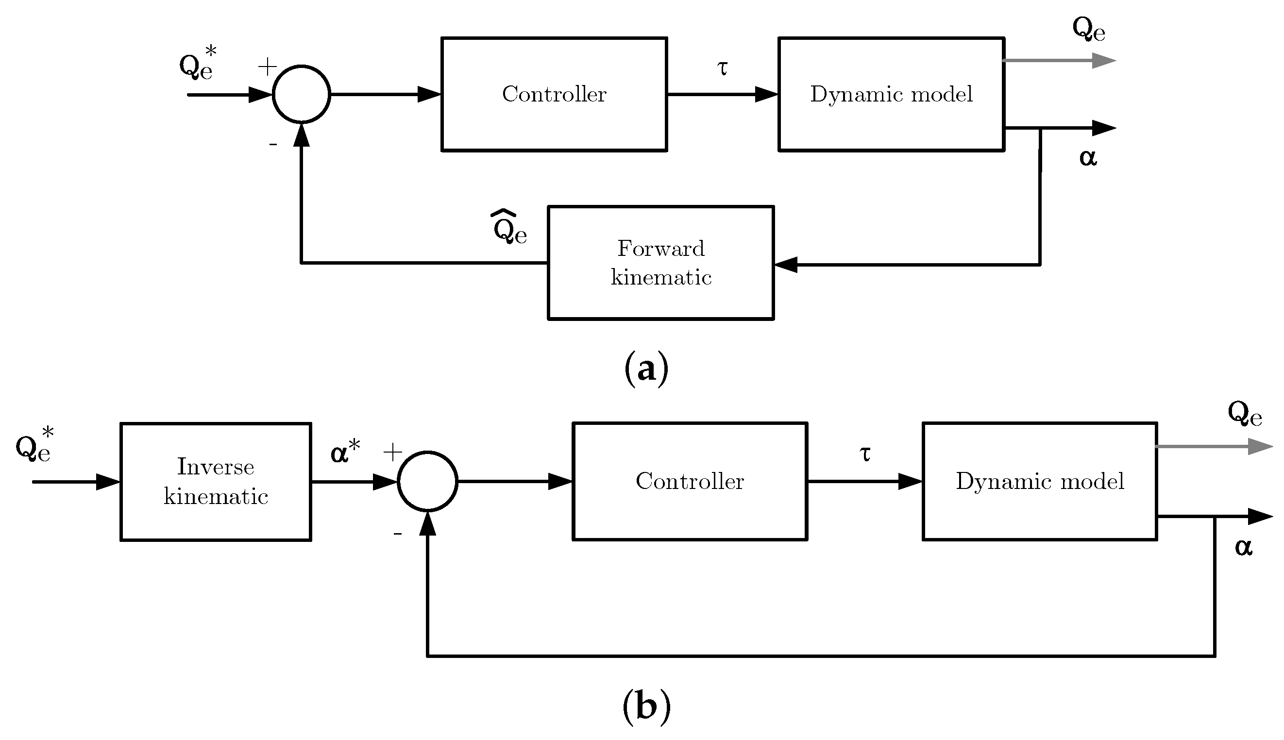
4.1. Control Scheme

One of the main control goals for a CDPR is to design a control scheme for end-effector positioning. This control approach shall achieve that the end-effector pose ${\mathbf{Q}}_e={[x_e,y_e,{\delta }_e]}^T$ follows a trajectory reference ${\mathbf{Q}}_e^{*}={[x_e^{*},y_e^{*},{\delta }_e^{*}]}^T$, but maintaining all cables’ tension in the allowed range $[T_{min},T_{max}]$.

Assuming that the measurable variables are the angular position of the motors, under an overall point of view, the CDPR can be controlled on Cartesian coordinates (${\mathbf{Q}}_e={[x_e,y_e,{\delta }_e]}^T$) or on joint coordinates ($\mathbf{\alpha }={[{\alpha }_1,{\alpha }_2,{\alpha }_3,{\alpha }_4]}^T$); this make reference to the variable that is used in the feedback loop of the control scheme. Figure 6 represents both control schemes.

Figure 6. Overall control approaches. (a) Cartesian coordinates’ space control; (b) joint coordinates’ space control.

Note that Cartesian coordinates’ control (Figure 6a) requires the estimation of the end-effector pose, ${\hat{\mathbf{Q}}}_e$, by means of the forward kinematics. In addition, the controller block receives a $3\times 1$ error signal and must output a $4\times 1$ control signal, and therefore, the controller block is a coupled $4\times 3$ matrix. This makes the control tuning difficult, and an uncoupling technique must be applied to obtain the controllers’ parameters (e.g., [46]).

On the contrary, the joint coordinates’ space control requires the inverse kinematics, for the joints’ reference generator, ${\mathbf{\alpha }}^{*}$, and the controller block is formed by a $4\times 4$ diagonal matrix, while SISO controllers can be tuned for each motor. For this reason, the joint coordinates’ space control was selected for the end-effector positioning control.

4.2. Trajectory Generation

The trajectory generation in our proposal is one of the main problems to be solved. Note that, for joint space control, the inverse kinematics is required, but it has infinite solutions. We can obtain a given ${\mathbf{Q}}_e^{*}=[x_e^{*},y_e^{*},{\delta }_e^{*}]$ with the infinity position of the lower and upper carriage position, $x_{lc}$ and $x_{uc}$, but most of then are not compatible with the dynamic model.

In this sense, together with the ${\mathbf{Q}}_e^{*}$ generation, it is required to also generate $x_{lc}^{*}$ and $x_{uc}^{*}$. In particular, the trajectory generator proposed here is based on the statically feasible workspace [42] and follows these steps:

(a)

Generation of the desired end-effector trajectory ${\mathbf{Q}}_{\mathbf{e}}^{*}$.

(b)

For a given ${\mathbf{Q}}_{\mathbf{e}}^{*}$, the tension value of one cable is fixed to $T_o^{*}$; in our case, $T_1$ was arbitrary set.

(c)

For the established values of ${\mathbf{Q}}_{\mathbf{e}}^{*}$ and $T_1=T_o^{*}$, the static equilibrium problem is solved to determine $x_{lc}^{*}$ and $x_{uc}^{*}$. To solve this problem, the Levenberg–Marquardt algorithm is applied [47].

The simulation results in Section 5 show that this trajectory-generation technique allows reaching a high-performance trajectory tracking of the end-effector.

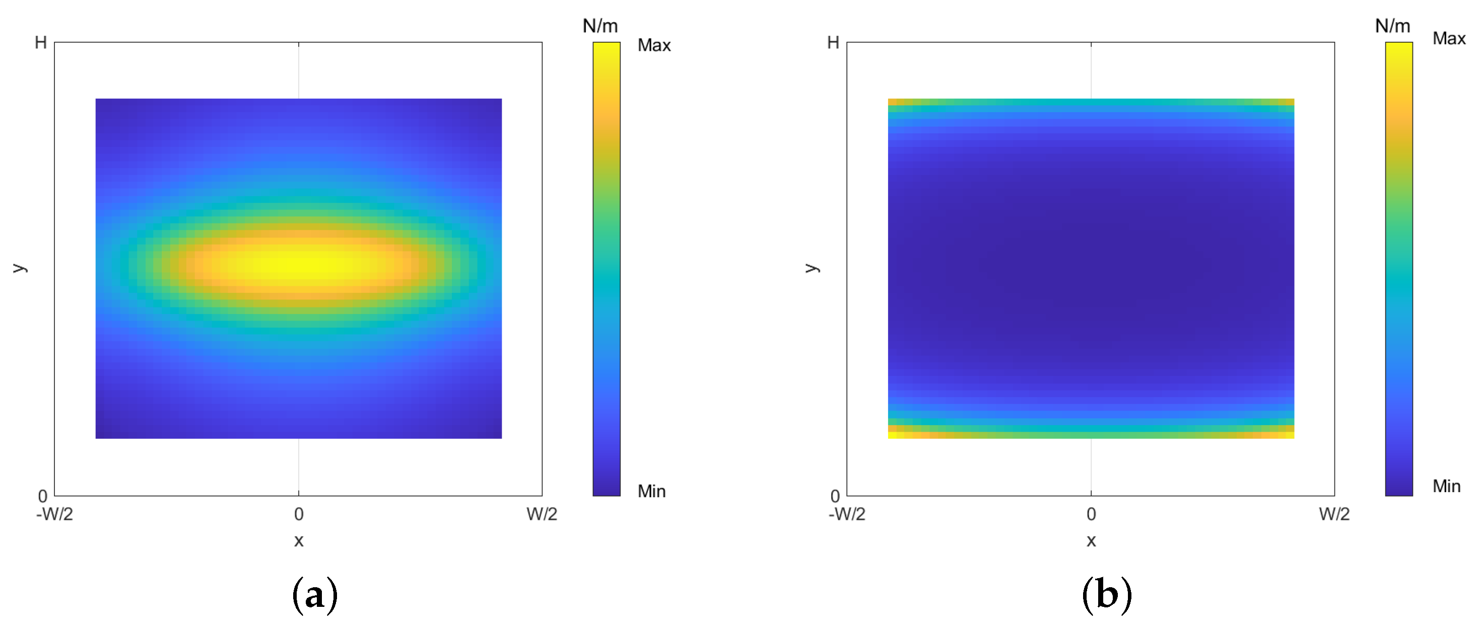
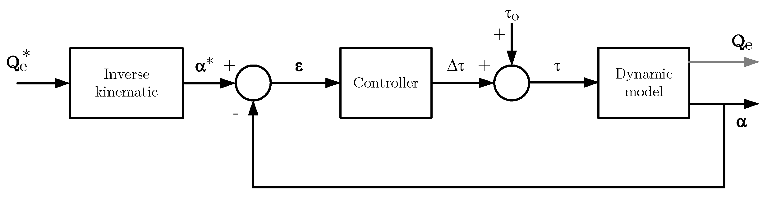
4.3. Positive Tension Problem and Vibration Rejection

Finally, we cannot forget the problem of maintaining cables’ tension within the allowed tension range $[T_{min},T_{max}]$. Owing to the fact that, in our proposal, the cable angles ${\theta }_i$ remain very close to $\pm \pi /2$ rad in almost all workspaces, a simple but effective modification of the control scheme shown in Figure 6b can be applied for maintaining the cables’ tension within the allowed range. Figure 7 presents this simple modification.

Figure 7. Final control approach for end-effector positioning.

It consists of adding a control signal offset, ${\mathbf{\tau }}_o$, to the control signal generated by the controller block, $\mathsf{\Delta }\mathbf{\tau }$. In this way, a new control signal is introduced to the system:

$$\mathbf{\tau }=\mathsf{\Delta }\mathbf{\tau }+{\mathbf{\tau }}_o$$

(18)

where ${\mathbf{\tau }}_o$ can be set, in a first approach, equal for all cables to a fixed value within the allowed tension range ${\mathbf{T}}_o^{*}\in [T_{min},T_{max}]$ multiplied by the winch pulley radius, $r_w$. The final control signal can be therefore written as:

$$\mathbf{\tau }=\mathsf{\Delta }\mathbf{\tau }+r_w{\mathbf{T}}_o^{*}$$

(19)

Finally, if a conventional PID controller is used for the end-effector positioning, the final control signal for commanding the CDPR is:

$$\mathbf{\tau }\left(t\right)={\mathbf{K}}_p\mathbf{\epsilon }\left(t\right)+{\mathbf{K}}_d\frac{d\mathbf{\epsilon }\left(t\right)}{dt}+{\mathbf{K}}_i{\int }_0^t\mathbf{\epsilon }\left(\sigma \right)d\sigma +r_w{\mathbf{T}}_o^{*}$$

(20)

$\mathbf{\epsilon }={\mathbf{\alpha }}^{*}-\mathbf{\alpha }$ being the error signal and ${\mathbf{K}}_p$, ${\mathbf{K}}_d$, and ${\mathbf{K}}_i$ diagonal matrices with the proportional, derivative, and integral constants of the controller, respectively. This controller constant can be obtained, for example, by tuning the regulator by means of the frequency domain or time domain techniques (e.g., [48]).

Without this offset control signal, ${\tau }_o$, a controller block to control the position of the joints can be easily found, but the tension of the four cables can reach negative values, so, as a consequence, this is not a valid solution in the real prototype. Actually, it is required to ensure not only that all tensions remain positive, but also $T_i>T_{min}$ for $i=1$ to 4, $T_{min}$ being the minimum tension allowed to avoid the sagging effect in the cables.

In this sense, many authors have proposed solving an optimisation problem, which results as the control signal to the motors, to guarantee that all tensions remain in the allowed range $[T_{min},T_{max}]$ [49]. Another extended tendency is to develop a force distribution algorithm [45], which can be applied for example to generate the trajectory tracking together with the control signal law [50]. Under our point of view, in the control of cable-driven parallel robots, the control scheme concept is more important that the particular controller technique (PID, sliding control, fuzzy controller, etc.).

After checking that the proposed control scheme can control the end-effector position and all tensions remain inside of the allowed range, we established the value of $T^{*}$ to minimise (or reject) the x axis vibration of the end-effector.

Although the inherent stiffness is not controlled by the cable tension, it has a significant impact on the system stiffness [51]. What is the system stiffness variation when $T^{*}$ changes? Can we, therefore, obtain a value of $T^{*}$ that rejects the x axis vibration of the end-effector, allowing a proper trajectory tracking? To answer this question, we changed the $T^{*}$ value from $T_{min}$ to $T_{max}$, and we executed horizontal rapid trajectories (worst case) and determined the amplitude and frequency of the end-effector when it reaches the steady state. Assuming an illustrative tension range of $[50,200]$ N for the cables’ tension, the result after executing the same trajectory, with the same PID controller, but different $T^{*}$ values, is shown in Figure 8.

Figure 8. Effect of $T^{*}$ on the vibration rejection.

In this sense, it is important to mention that the higher $T^{*}$, the higher the frequency of the vibration is and the lower is the amplitude. In this sense, the simulation results of the following section show that the non-desirable vibration of the end-effector owing to its low horizontal stiffness can be easily rejected by increasing the $T_o^{*}$ value within the $[T_{min},T_{max}]$ range.

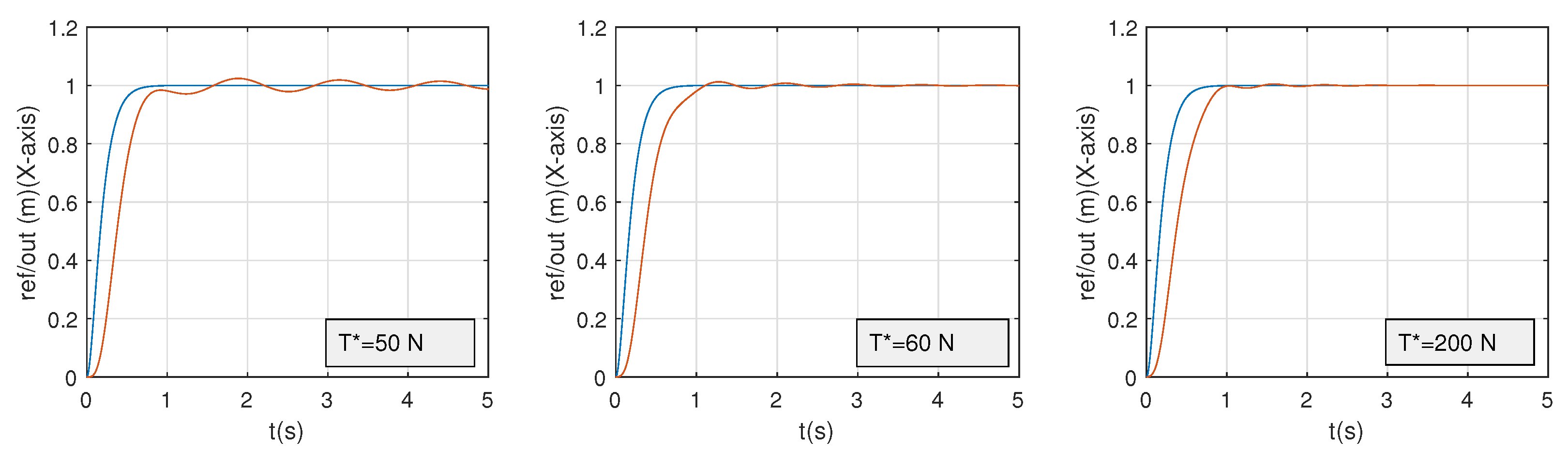
4.4. Controller Tuning

The PID controller has three parameters to be tuned, $K_p$, $K_i$, and $K_d$. As Dynamic Model (16) is non-linear, some linearisation technique must be used for tuning the controller. The most-applied linearisation techniques are: feedback linearisation and removing the non-linear part near an equilibrium point. If we look at some works where PID control is used (e.g., [52]), most of them finally select values of the controller gains to ensure the stability, but no linear technique is described to analytically obtain the gains.

In our case, owing to the cables’ angle changing much less than the conventional scheme during end-effector movement (see ${\theta }_i$ in Figure 2), the non-linear effect is lower than in the conventional CDPRs, and we can directly remove the non-linear term of the dynamic model to assume an LTI model, which corresponds to the model of a DC motor, and then, apply linear tuning methods for the ID controller, in our case the frequency domain technique.

Assuming the corresponding linear transfer function of one joint, $G\left(s\right)$, the PID controller was tuned by a simple frequency domain technique based on defining the gain crossover frequency, ${\omega }_c$, and phase margin, ${\phi }_m$, of the equivalent open-loop transfer function system. The complex equation to obtain the controllers’ parameters is [48]:

$$R\left(j{\omega }_c\right)G\left(j{\omega }_c\right)=-e^{j{\phi }_m}$$

(21)

The controller parameters can be therefore easily obtained with this tuning equation:

$$K_p=\Re \left\{\frac{-cos\left({\phi }_m\right)-jsin\left({\phi }_m\right)}{G\left(j{\omega }_c\right)}\right\}$$

(22)

$$K_d=\frac{1}{{\omega }_c}\left(-\frac{K_i}{{\omega }_c}+\Im \left\{\frac{-cos\left({\phi }_m\right)-jsin\left({\phi }_m\right)}{G\left(j{\omega }_c\right)}\right\}\right)$$

(23)

where $\Re \left\{\right\}$ and $\Im \left\{\right\}$ are the real and imaginary parts and $K_i$ can be selected to minimise the influence of the non-linear term of the dynamics model, for example minimising the tracking error by means of simulations.

5. Simulation Results

5.1. Preliminaries

This section validates the control approach by executing several simulated trajectories using Matlab${}^{\circledR }$ and Simulink${}^{\circledR }$. A fixed sample time of 1 ms was set while using the ode4 (Runge–Kutta) solver. Table 1 summarises the parameters used for the simulations.

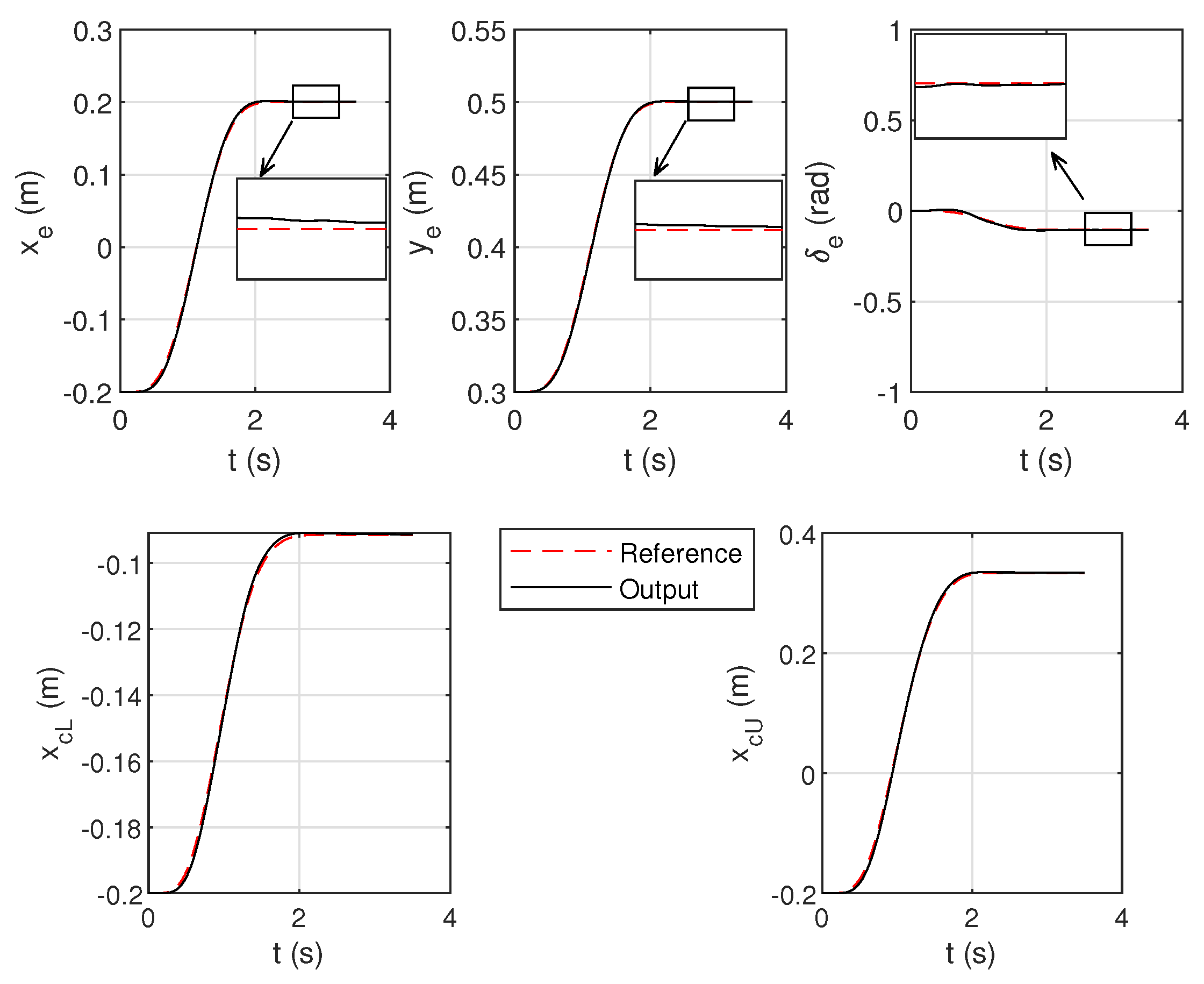
5.2. Control Approach Validation

One of the main drawbacks of the new design is the loss of stiffness along the x direction. This leads to non-desirable end-effector vibrations while executing manoeuvres. In order to validate the proposed control, several trajectories were executed while monitoring the end-effector and carriage positions and the cable tensions. Dynamic Model (16) is a second-order system, and the fifth Bezier trajectories were implemented to ensure smooth trajectories while avoiding abrupt changes in the control signal values, which can lead, once again, to non-desirable end-effector vibrations.

For illustrative purpose, a set of trajectories was executed with zero end-effector orientation. In addition, the last trajectory was executed while orienting the end-effector, proving that the control is capable of avoiding non-desirable vibrations, even with more complex manoeuvres. Note that, for all cases of study, the end-effector tracks the reference during all the trajectory. The average trajectory tracking error, $e_a$, is estimated by:

$$e_a=\frac{{\sum }_{i=1}^N\left|\right|{\mathbf{Q}}_e^{*}-{\mathbf{Q}}_e{\left|\right|}_2}{N}$$

(24)

N being the number of samples of the simulation:

• Case I: Figure 9 shows a diagonal trajectory from initial pose ${\mathbf{Q}}_e^0=[-0.2,0.3,0]$ to ${\mathbf{Q}}_e=[0.2,0.5,0]$. The average error (24) of the executed trajectory is $1.45\times {10}^{-4}$ m-rads.
  

  Figure 9. Case I results.
• Case II: Figure 10 shows a reorientation trajectory from initial pose ${\mathbf{Q}}_e^0=[0,0.4,0]$ to ${\mathbf{Q}}_e=[0,0.4,6]$. The average error (24) of the executed trajectory is $4.02\times {10}^{-4}$ m-rads.
  

  Figure 10. Case II results.
• Case III: Figure 11 presents a diagonal trajectory from initial pose ${\mathbf{Q}}_e^0=[-0.2,0.3,0]$ to ${\mathbf{Q}}_e=[0.2,0.5,-6]$. This trajectory introduces a change in the end-effector orientation while executing the diagonal movement. The average error (24) of the executed trajectory is $2.17\times {10}^{-4}$ m-rads.
  

  Figure 11. Case III results.

These three cases were simulated for an allowed tension range, $[10,100]$, and the reference tension, $T_o^{*}$, to determine that the control signal output has been fixed to 50 N. Figure 12 represents the tension of the cables for Cases I, II, and III. Note that the cables’ tensions remain within the allowed range of tensions.

Figure 12. Cable tensions: Cases I, II, and III.

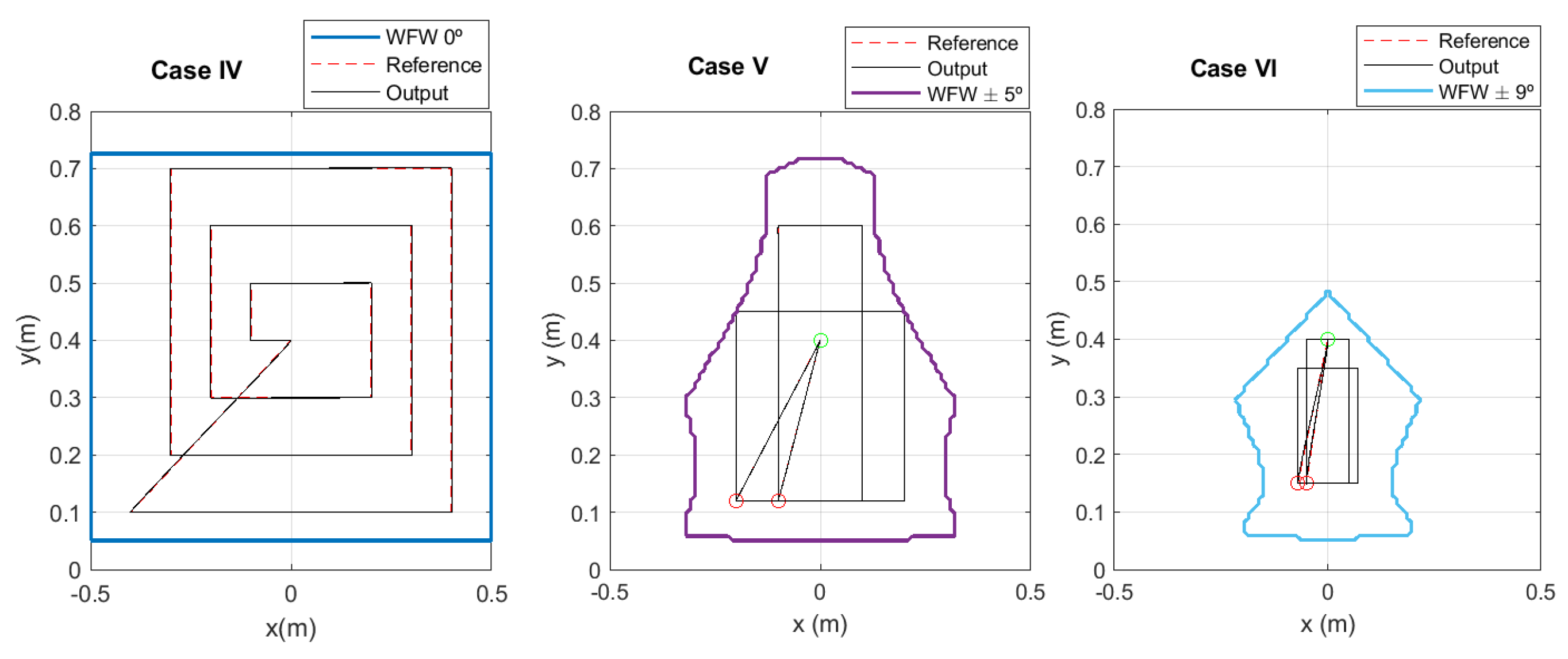
5.3. WFW Increase Validation

As mentioned previously, this novel design increases the WFW in comparison to the conventional CPDR scheme. In this sense, more frame area could be covered while executing manoeuvres. It should be pointed out that the oriented WFW of the novel design is also bigger than the one of a conventional CDPR (see Figure 3).

In order to validate this, a multi-line trajectory near the WFW limits shown in Figure 3b with different end-effector orientations was executed. In particular, the case of studies are as follows:

• Case IV: The orientation of the end-effector is fixed at ${\delta }_e=0^{\circ }$. The multi-line trajectory tracking results are shown in Figure 13—Case IV. The average error (24) of the executed trajectory is $3.87\times {10}^{-4}$ m-rads.
  

  Figure 13. Results of Cases IV, V, and VI.
• Case V: The orientation of the end-effector was fixed to ${\delta }_e=-5^{\circ }$. The trajectory tracking results are shown in Figure 13—Case V. The average error (24) of the executed trajectory is $1.98\times {10}^{-4}$ m-rads.
• Case VI: The orientation of the end-effector was fixed to ${\delta }_e=9^{\circ }$. The trajectory tracking results are shown in Figure 13. The average error (24) of the executed trajectory is $4.81\times {10}^{-4}$ m-rads.

In Figure 13, the circle in green represents the initial position of the trajectory and red ones the final positions.

It is notable that, in the three cases of study, the selected trajectory covers a great area of its corresponding maximum WFW (see Figure 3). In addition, the cable tensions for Cases IV, V, and VI also remain within the allowed range of tensions. The results obtained in this section allowed the authors to validate both the control approach and the WFW increase.

6. Experimental Results

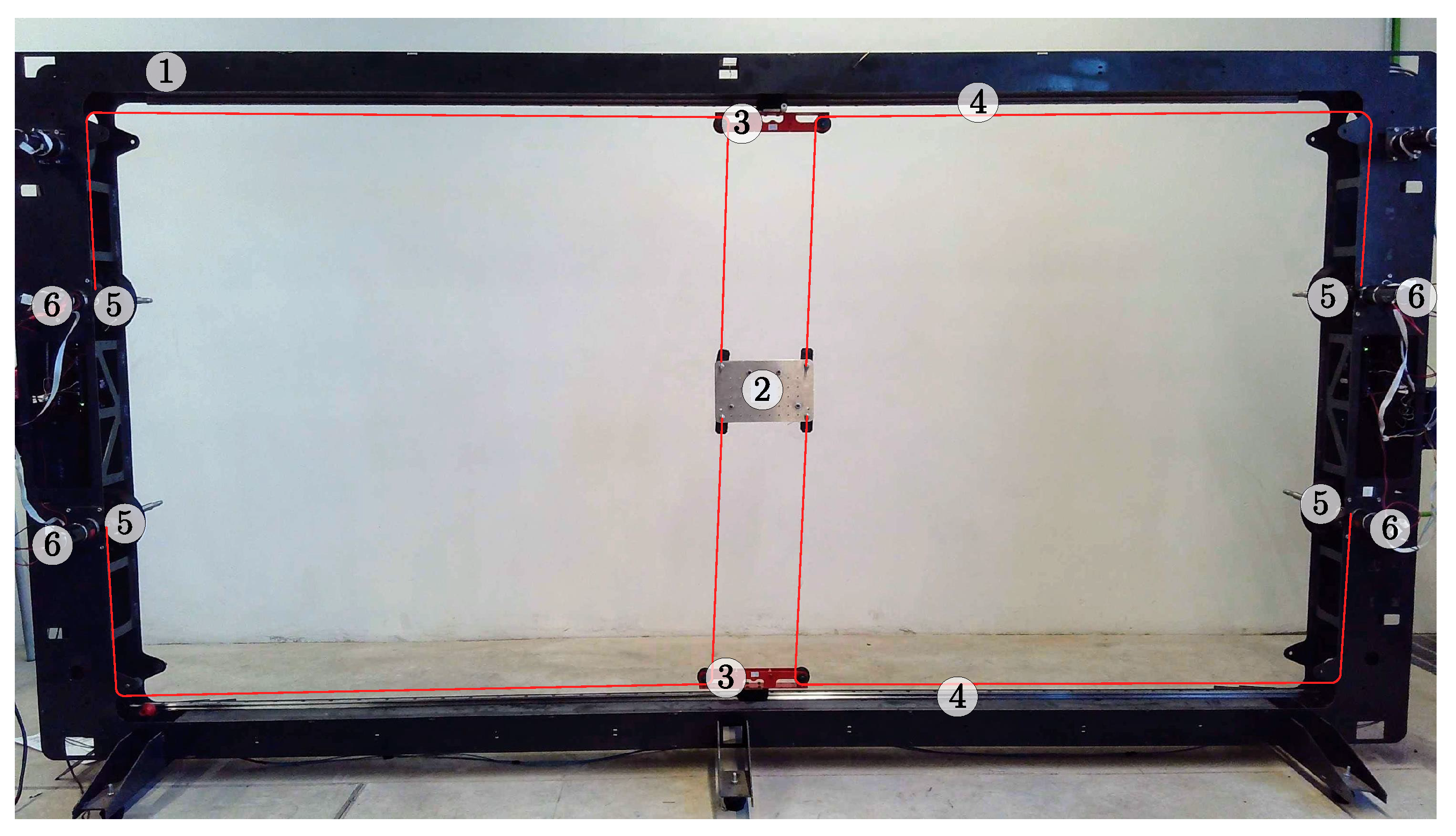
6.1. Preliminaries

The proposal here is experimentally validated by means of the prototype shown in Figure 14, where the main functional elements are: ① frame; ② end-effector; ③ carriages; ④ linear guides; ⑤ winches; ⑥ DC motors. In Figure 14, the cable path is coloured in red for illustrative purposes. The main parameters of the robot are summarised in Table 2.

Figure 14. Prototype.

Table 2. Prototype parameters.

Subsystem	Parameter	Value
Frame	H	$1.2$ m
	W	$2.0$ m
Carriages	$w_{cl}$	$0.21$ m
	$w_{cu}$	$0.21$ m
	$m_c$	$1.26$ kg
	$b_c$	$0.2$ Ns/m
	$r_c$	$0.01$ m
Motor/winch set	J	$4.61\times {10}^{-4}$ Kgm${}^2$
	$b_m$	$7.69\times {10}^{-3}$ Nms
	r	$0.06$ m
End-effector	$m_e$	$1.8$ kg
	w	$0.18$ m
	h	$0.11$ m
	$I_e$	$2\times {10}^{-3}$ Kgm${}^2$

The joint coordinates of the motors, Maxon RE40 DC Motors, are controlled by means of servo amplifiers, ESCON 70/10, which receive the control signal from the control equipment. This control device is a Ni MyRio 1900 real-time controller, which is able to maintain a sample time of 1 ms during all the manoeuvres. The controllers’ parameters were tuned using a gain crossover frequency ${\omega }_c=40$ rad/s and a phase margin ${\phi }_m={60}^{\circ }$, which yield the controller parameters: $K_p=0.6891$, $K_i=0.57$, and $K_d=0.0102$.

The end-effector and the carriages’ poses were obtained by recording the movement with an IP-evo 4K camera with a resolution of $3264\times 2448$ and a frame rate of 30 frames per second. The videos were processed offline with Matlab${}^{\mathrm{TM}}$ to detect the position of a reflector located on the points of interest.

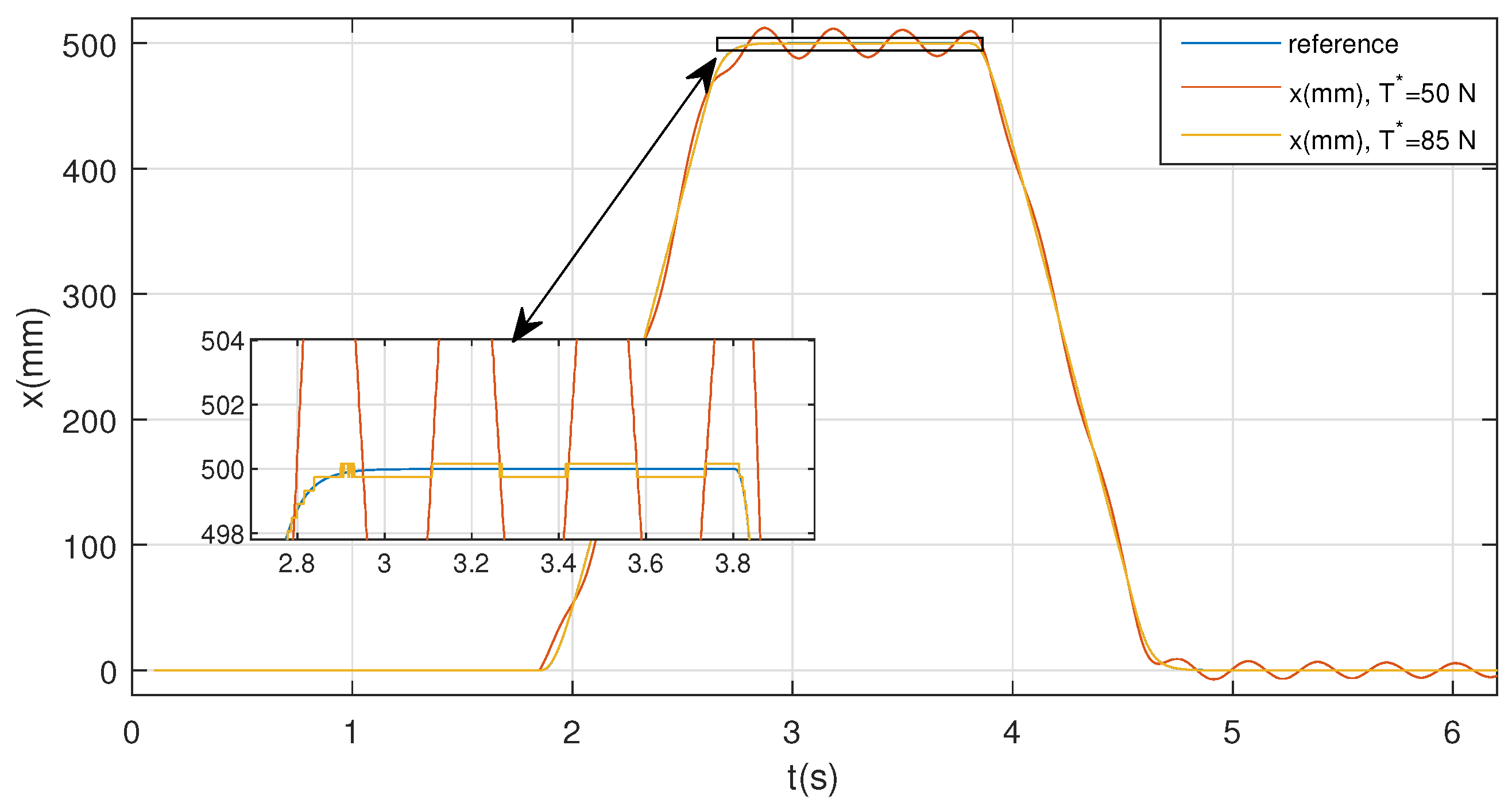
6.2. Trajectory Tracking

In order to experimentally validate the proposal, a horizontal trajectory (worst case) was tested with a length of $0.500$ m, maintaining the orientation at $0^{\circ }$. Figure 15 shows the results for $T^{*}=50$ and 85 N in order to illustrate the influence of the control signal offset, ${\tau }_o$, in the trajectory tracking.

Figure 15. Trajectory tracking of horizontal manoeuvres with different values of $T^{*}$.

Note how a greater $T^{*}$ lowers the amplitude of the end-effector vibration, but a compromise between the $T^{*}$ value and control signal saturation must be stated to avoid the actuator saturation. Figure 16 represents the tracking error for both cases. Note that the maximum error for $T^{*}=50$ N is about 16 mm, since for $T^{*}=85$ N, it is about 0.5 mm.

Figure 16. Tracking error of horizontal manoeuvres with different values of $T^{*}$.

7. Conclusions

This paper proposed a new dynamic control technique for a novel CDPR design. This novel design is based in the addition of passive carriages to the robot frame of a 3DOF CDPR. The main goal of the new concept is to increase the robot WFW because of the smaller change in the cable directions.

As the main disadvantage of the new design is the loss of stiffness in the x direction, one of the goals of the new dynamic control technique was to minimise the vibrations originated in this direction, ensuring an accurate trajectory tracking.

The kinematic and dynamic equations of the robot were presented in order to select an appropriate control approach for the implemented dynamic model.

The control strategy presented tackles with the trajectory generation, the positive tension problem, and the vibration rejection. This control approach is based on the addition of an offset control signal.

In order to validate the dynamic control, several tracking trajectories for the end-effector were simulated. The average error always remained lower than 1 mm, and a good avoidance of vibrations was accomplished. In addition, to assess the improvement of the WFW while validating the novel control, a set of different trajectories was used for several end-effector orientations. The results showed how the new design together with the proposed control allowed the CDPR to manoeuvre in a much larger area with good dexterity.

For experimental validation, a horizontal trajectory (worst case) was executed for two values of $T^{*}$ to illustrate how the offset control signal value can reject the vibration of the end-effector along the horizontal axis.

References

- Merlet, J.P. Parallel Robots; Springer Science & Business Media: Berlin/Heidelberg, Germany, 2005; Volume 128. [Google Scholar]
- Bosscher, P.; Williams, R.L.; Tummino, M. A concept for rapidly-deployable cable robot search and rescue systems. In Proceedings of the International Design Engineering Technical Conferences and Computers and Information in Engineering Conference, Long Beach, CA, USA, 24–28 September 2005; Volume 47446, pp. 589–598. [Google Scholar]
- Tadokoro, S.; Verhoeven, R.; Hiller, M.; Takamori, T. A portable parallel manipulator for search and rescue at large-scale urban earthquakes and an identification algorithm for the installation in unstructured environments. In Proceedings of the 1999 IEEE/RSJ International Conference on Intelligent Robots and Systems, Human and Environment Friendly Robots with High Intelligence and Emotional Quotients (Cat. No. 99CH36289), Kyongju, Republic of Korea, 17–21 October 1999; Volume 2, pp. 1222–1227. [Google Scholar]
- Ottaviano, E.; Ceccarelli, M.; De Ciantis, M. A 4–4 cable-based parallel manipulator for an application in hospital environment. In Proceedings of the 2007 Mediterranean Conference on Control & Automation, Athens, Greece, 27–29 June 2007; pp. 1–6. [Google Scholar]
- Gallina, P.; Rosati, G. Manipulability of a planar wire driven haptic device. Mech. Mach. Theory 2002, 37, 215–228. [Google Scholar] [CrossRef]
- Skycam. Available online: http://www.skycam.tv/2022 (accessed on 10 October 2022).
- Gueners, D.; Chanal, H.; Bouzgarrou, B.C. Design and implementation of a cable-driven parallel robot for additive manufacturing applications. Mechatronics 2022, 86, 102874. [Google Scholar] [CrossRef]
- Castelli, G.; Ottaviano, E.; Rea, P. A Cartesian Cable-Suspended Robot for improving end-users’ mobility in an urban environment. Robot.-Comput.-Integr. Manuf. 2014, 30, 335–343. [Google Scholar] [CrossRef]
- Kawamura, S.; Choe, W.; Tanaka, S.; Kino, H. Development of an ultrahigh speed robot FALCON using parallel wire drive systems. J. Robot. Soc. Jpn. 1997, 15, 82–89. [Google Scholar] [CrossRef]
- Gonzalez-Rodriguez, A.; Castillo-Garcia, F.; Ottaviano, E.; Rea, P.; Gonzalez-Rodriguez, A. On the effects of the design of cable-Driven robots on kinematics and dynamics models accuracy. Mechatronics 2017, 43, 18–27. [Google Scholar] [CrossRef]
- Albus, J.; Bostelman, R.; Dagalakis, N. The NIST robocrane. J. Robot. Syst. 1993, 10, 709–724. [Google Scholar] [CrossRef]
- Duan, B.; Qiu, Y.; Zhang, F.; Zi, B. Analysis and experiment of the feed cable-suspended structure for super antenna. In Proceedings of the 2008 IEEE/ASME International Conference on Advanced Intelligent Mechatronics, Xi’an, China, 2–5 July 2008; pp. 329–334. [Google Scholar]
- Tho, T.P.; Thinh, N.T. An Overview of Cable-Driven Parallel Robots: Workspace, Tension Distribution, and Cable Sagging. Math. Probl. Eng. 2022, 2022, 2199748. [Google Scholar] [CrossRef]
- Abbasnejad, G.; Carricato, M. Direct geometrico-static problem of underconstrained cable-driven parallel robots with n cables. IEEE Trans. Robot. 2015, 31, 468–478. [Google Scholar] [CrossRef]
- Castelli, G.; Ottaviano, E.; González, A. Analysis and simulation of a new Cartesian cable-suspended robot. Proc. Inst. Mech. Eng. Part J. Mech. Eng. Sci. 2010, 224, 1717–1726. [Google Scholar] [CrossRef]
- Idà, E.; Bruckmann, T.; Carricato, M. Rest-to-rest trajectory planning for underactuated cable-driven parallel robots. IEEE Trans. Robot. 2019, 35, 1338–1351. [Google Scholar] [CrossRef]
- Gouttefarde, M.; Gosselin, C.M. Analysis of the wrench-closure workspace of planar parallel cable-driven mechanisms. IEEE Trans. Robot. 2006, 22, 434–445. [Google Scholar] [CrossRef]
- Gouttefarde, M.; Daney, D.; Merlet, J.P. Interval-analysis-based determination of the wrench-feasible workspace of parallel cable-driven robots. IEEE Trans. Robot. 2010, 27, 1–13. [Google Scholar] [CrossRef]
- Kozak, K.; Zhou, Q.; Wang, J. Static analysis of cable-driven manipulators with non-negligible cable mass. IEEE Trans. Robot. 2006, 22, 425–433. [Google Scholar] [CrossRef]
- Riehl, N.; Gouttefarde, M.; Krut, S.; Baradat, C.; Pierrot, F. Effects of non-negligible cable mass on the static behavior of large workspace cable-driven parallel mechanisms. In Proceedings of the 2009 IEEE International Conference on Robotics and Automation, Kobe, Japan, 12–17 May 2009; pp. 2193–2198. [Google Scholar]
- Merlet, J.P. The kinematics of cable-driven parallel robots with sagging cables: Preliminary results. In Proceedings of the 2015 IEEE International Conference on Robotics and Automation (ICRA), Seattle, WA, USA, 26–30 May 2015; pp. 1593–1598. [Google Scholar]
- Ottaviano, E.; Arena, A.; Gattulli, V. Geometrically exact three-dimensional modeling of cable-driven parallel manipulators for end-effector positioning. Mech. Mach. Theory 2021, 155, 104102. [Google Scholar] [CrossRef]
- Du, J.; Bao, H.; Cui, C.; Yang, D. Dynamic analysis of cable-driven parallel manipulators with time-varying cable lengths. Finite Elem. Anal. Des. 2012, 48, 1392–1399. [Google Scholar] [CrossRef]
- Kawamura, S.; Kino, H.; Won, C. High-speed manipulation by using parallel wire-driven robots. Robotica 2000, 18, 13–21. [Google Scholar] [CrossRef]
- Zi, B.; Duan, B.; Du, J.; Bao, H. Dynamic modeling and active control of a cable-suspended parallel robot. Mechatronics 2008, 18, 1–12. [Google Scholar] [CrossRef]
- Bruckmann, T.; Sturm, C.; Lalo, W. Wire robot suspension systems for wind tunnels. In Wind Tunnels and Experimental Fluid Dynamics Research; IntechOpen: London, UK, 2010; pp. 29–50. [Google Scholar]
- Oh, S.R.; Agrawal, S. A reference governor-based controller for a cable robot under input constraints. IEEE Trans. Control. Syst. Technol. 2005, 13, 639–645. [Google Scholar] [CrossRef]
- Ma, O.; Diao, X. Dynamics analysis of a cable-driven parallel manipulator for hardware-in-the-loop dynamic simulation. In Proceedings of the 2005 IEEE/ASME International Conference on Advanced Intelligent Mechatronics, Monterey, CA, USA, 24–28 July 2005; pp. 837–842. [Google Scholar]
- Du, J.; Ding, W.; Bao, H. Cable vibration analysis for large workspace cable-driven parallel manipulators. In Cable-Driven Parallel Robots; Springer: Berlin/Heidelberg, Germany, 2013; pp. 437–449. [Google Scholar]
- Diao, X.; Ma, O. Vibration analysis of cable-driven parallel manipulators. Multibody Syst. Dyn. 2009, 21, 347–360. [Google Scholar] [CrossRef]
- Behzadipour, S.; Khajepour, A. Stiffness of cable-based parallel manipulators with application to stability analysis. J. Mech. Des. 2006, 128, 303–310. [Google Scholar] [CrossRef]
- Tempel, P.; Miermeister, P.; Lechler, A.; Pott, A. Modelling of kinematics and dynamics of the IPAnema 3 cable robot for simulative analysis. Appl. Mech. Mater. 2015, 794, 419–426. [Google Scholar] [CrossRef]
- Yuan, H.; Courteille, E.; Deblaise, D. Static and dynamic stiffness analyses of cable-driven parallel robots with non-negligible cable mass and elasticity. Mech. Mach. Theory 2015, 85, 64–81. [Google Scholar] [CrossRef]
- Wu, Q.; Takahashi, K.; Nakamura, S. Formulae for frequencies and modes of in-plane vibrations of small-sag inclined cables. J. Sound Vib. 2005, 279, 1155–1169. [Google Scholar] [CrossRef]
- Zhou, X.; Yan, S.; Chu, F. In-plane free vibrations of an inclined taut cable. J. Vib. Acoust. 2011, 133, 031001. [Google Scholar] [CrossRef]
- Du, J.; Cui, C.; Bao, H.; Qiu, Y. Dynamic Analysis of Cable-Driven Parallel Manipulators Using a Variable Length Finite Element. J. Comput. Nonlinear Dyn. 2014, 10, 011013. [Google Scholar] [CrossRef]
- Meunier, G.; Boulet, B.; Nahon, M. Control of an overactuated cable-driven parallel mechanism for a radio telescope application. IEEE Trans. Control Syst. Technol. 2009, 17, 1043–1054. [Google Scholar] [CrossRef]
- Pott, A. Cable-Driven Parallel Robots: Theory and Application; Springer: Cham, Switzerland, 2018. [Google Scholar]
- Martin-Parra, A.; Juarez-Perez, S.; Gonzalez-Rodriguez, A.; Gonzalez-Rodriguez, A.G.; Lopez-Diaz, A.I.; Rubio-Gomez, G. A novel design for fully constrained planar Cable-Driven Parallel Robots to increase their wrench-feasible workspace. Mech. Mach. Theory 2023, 180, 105159. [Google Scholar] [CrossRef]
- Youssef, K.; Otis, M.J.D. Reconfigurable fully constrained cable driven parallel mechanism for avoiding interference between cables. Mech. Mach. Theory 2020, 148, 103781. [Google Scholar] [CrossRef]
- Rushton, M.; Khajepour, A. Planar variable structure cable-driven parallel robots for circumventing obstacles. J. Mech. Robot. 2021, 13, 021011. [Google Scholar] [CrossRef]
- Trevisani, A. Planning of dynamically feasible trajectories for translational, planar, and underconstrained cable-driven robots. J. Syst. Sci. Complex. 2013, 26, 695–717. [Google Scholar] [CrossRef]
- Pott, A. Geometric and Static Foundations. In Cable-Driven Parallel Robots; Springer: Berlin/Heidelberg, Germany, 2018; pp. 45–117. [Google Scholar]
- Moradi, A. Stiffness Analysis of Cable-Driven Parallel Robots; Queen’s University: Kingston, ON, Canada, 2013. [Google Scholar]
- Pott, A. An improved force distribution algorithm for over-constrained cable-driven parallel robots. In Computational Kinematics; Springer: Dordrecht, The Netherlands, 2014; pp. 139–146. [Google Scholar]
- Lieslehto, J. MIMO controller design using SISO controller design methods. IFAC Proc. Vol. 1996, 29, 1152–1156. [Google Scholar] [CrossRef]
- Ranganathan, A. The levenberg-marquardt algorithm. Tutoral LM Algorithm 2004, 11, 101–110. [Google Scholar]
- Ogata, K. Modern Control Engineering; Pearson: Upper Saddle River, NJ, USA, 2010; Volume 5. [Google Scholar]
- Zhang, B.; Shang, W.; Cong, S.; Li, Z. Coordinated dynamic control in the task space for redundantly actuated cable-driven parallel robots. IEEE/ASME Trans. Mechatron. 2020, 26, 2396–2407. [Google Scholar] [CrossRef]
- Yuan, H.; Courteille, E.; Deblaise, D. Force distribution with pose-dependent force boundaries for redundantly actuated cable-driven parallel robots. J. Mech. Robot. 2016, 8, 041004. [Google Scholar] [CrossRef]
- Cui, Z.; Tang, X.; Hou, S.; Sun, H. Research on controllable stiffness of redundant cable-driven parallel robots. IEEE/ASME Trans. Mechatron. 2018, 23, 2390–2401. [Google Scholar] [CrossRef]
- Khosravi, M.A.; Taghirad, H.D. Robust PID control of fully-constrained cable driven parallel robots. Mechatronics 2014, 24, 87–97. [Google Scholar] [CrossRef]