Integrated Propulsion and Cabin-Cooling Management for Electric Vehicles

Abstract

This paper presents two nonlinear model predictive control (MPC) methods for the integrated propulsion and cabin-cooling management of electric vehicles. An air-conditioning (AC) model, which has previously been validated on a real system, is used to accomplish system-level optimization. To investigate the optimal solution for the integrated optimal control problem (OCP), we first build an MPC, referred to as a joint MPC, in which the goal is to minimize battery energy consumption while maintaining cabin-cooling comfort. Second, we divide the integrated OCP into two small-scale problems and devise a co-optimization MPC (co-MPC), where speed planning on hilly roads and cabin-cooling management with propulsion power information are addressed successively. Our proposed MPC methods are then validated through two case studies. The results show that both the joint MPC and co-MPC can produce significant energy benefits while maintaining driving and thermal comfort. Compared to regular constant-speed cruise control that is equipped with a proportion integral (PI)-based AC controller, the benefits to the battery energy earned by the joint MPC and co-MPC range from 2.09% to 2.72%. Furthermore, compared with the joint MPC, the co-MPC method can achieve comparable performance in energy consumption and temperature regulation but with reduced computation time.

1. Introduction

The electrification of vehicles has become an unstoppable force due to severe environmental pollution and a shortage of fossil fuel resources [1,2]. Compared to hybrid electric vehicles (HEVs), electric vehicles (EVs) have higher energy efficiency and can realize zero emissions. With their superior performance, EVs are becoming more attractive to automotive manufacturers and consumers [3]. Nonetheless, the well-known range anxiety caused by limited battery capacity remains a concern for further establishing their mass-market acceptance [4]. Therefore, improving overall energy efficiency and saving energy are essential for EVs.

Eco-driving is the main method of increasing the efficiency of EVs. Based on terrain data obtained from vehicle-to-infrastructure (V2I) or geographical information systems (GIS), the eco-driving controller can determine the optimal energy-saving velocity profile along a certain route [5,6,7]. Several methods have been proposed in the past to address this topic. Dynamic programming (DP), also known as the globally optimal method, is widely used as a benchmark strategy but is not suited for real-time applications due to its computational burden [8,9,10]. Another popular method is Pontryagin’s maximum principle (PMP), which has been demonstrated to be successful in addressing real-time energy management in HEVs [11]. Yet, for speed planning on hilly roads, the PMP method is still burdened with a high computational load or is too complex to implement [12]. In addition, heuristic-based feedback control methods have been proposed, but these rely heavily on parameter tuning, and their performance may deteriorate in various driving situations [13]. Recently, reinforcement learning (RL) methods have also been adopted for eco-driving [14]. RL is very similar to DP in that it can optimize the cost-to-go value function based on the Bellman equation. Unlike DP, RL introduces approximations to improve computational efficiency and thus can be used as a real-time controller [15]. The drawbacks of RL are the difficulty of designing a good reward function and balancing ‘exploration’ and ‘exploitation’, which can cause the algorithm to easily become trapped in a local optimum [16]. To take into account both the optimization performance and computational efficiency, model predictive control (MPC) has been proposed [17,18,19]. A two-level MPC method was presented in [20] to solve the cruise problem for a parallel HEV. The case study demonstrated that MPC is a suitable method for HEV energy management and cruise control.

However, the aforementioned eco-driving studies only dealt with the propulsion system. The power consumption of the heating, ventilation, and air conditioning (HVAC) was not considered. In fact, the HVAC system can contribute up to 20% of a vehicle’s energy consumption in hot or cold environments [21,22]. Several studies have been conducted to incorporate cabin thermal management into the power management of a single vehicle or multiple connected and automated vehicles. A battery lifetime-aware automotive climate control methodology was developed in [23] for an EV. However, this study adopted a low-order air-conditioning (AC) model that limited the model’s accuracy and caused variations in the controller’s performance for different drive profiles and ambient temperatures. A more accurate control-oriented AC system predictive model was described in [24]. With this model, an eco-cooling control method for a vehicle’s AC system was developed, incorporating the vehicle speed profile [25,26]. Similar studies and methods can be found in [27,28,29], where vehicle speed and traffic preview predictions over short and long prediction horizons were exploited. To consolidate the performance of these MPCs, two different multi-level MPC methods were proposed in [30,31]. Focusing on real-time computation, a linear time-varying MPC method was developed in [32] for an AC model with an ideal vapor-compression cycle. It can be concluded that most state-of-art AC control methods are usually designed to minimize AC power consumption under the assumption that speed profiles are known in advance. However, this is not always a reliable assumption. For example, a vehicle’s speed may vary depending on the speed limits, topography, and surrounding traffic. Meanwhile, the predicted speed can be further optimized to achieve eco-driving. Thus, instead of estimating the future speed, it would be more practical to optimally regulate the future speed.

To the best of the authors’ knowledge, eco-driving and HVAC management have not been considered together in an optimal control problem (OCP). In this paper, we study the integrated optimal control of eco-driving and cabin-cooling management using the MPC method. The main contributions are highlighted as follows:

• A joint optimization-based MPC is proposed to address the integration problem of eco-driving and thermal management. In order to achieve cabin thermal comfort, we introduce a novel state that constrains the average temperature over a moving window, thus ensuring fairness in the assessment of energy savings;
• A co-optimization-based MPC is subsequently proposed in order to produce comparable performance with a lower computational load;
• A detailed analysis is conducted in which the proposed MPC methods are compared to other benchmark control methods and their practicability is examined.

The remainder of this paper is organized as follows: Section 2 presents the system modeling including the control-oriented modeling of AC-level optimization and its validation. Section 3 uses the MPC method to formulate the optimization problem in both a global and distributed manner. The simulation setup and results of the case studies are presented in Section 4. Section 5 provides the performance evaluation of the proposed MPC methods. Finally, the concluding remarks are given in Section 6.

2. System Modeling

The overall power consumption of an EV, in which the battery is the main energy supplier, is categorized into three types: the propulsion motor, air-conditioning (AC) system, and vehicle ancillaries. Compared to the other two types, the ancillaries’ load is marginal and ignored in this study [33]. The modeling of the propulsion system as a part of the longitudinal dynamics of the vehicle, as well as the AC and battery system, are presented in this section. The schematic of the overall EV system is depicted in Figure 1. As shown in the figure, the EV system consists of a propulsion system, an AC system, and a cabin thermal system. Both the propulsion and AC systems are powered by the battery pack that is passively cooled by ambient air. The AC system has two operating modes, fresh air and recirculation. The cabin air temperature is influenced by the vented air into the cabin, the heat exchange with the cabin shell, and the cabin interior.

2.1. Vehicle Longitudinal Dynamics

Driving on a hilly road while achieving a certain kinetic and potential energy, the vehicle encounters retarding forces that include gradient resistance, rolling resistance, and air drag. The longitudinal dynamics schematic is illustrated in Figure 2, where m, $k_{\mathrm{f}}$, r, and g are the vehicle mass, final reduction ratio, wheel radius, and gravity acceleration, respectively; f is the rolling friction coefficient; and $\alpha \left(s\right)$ denotes the road slope at location s. The parameters $C_{\mathrm{D}}$, $A_{\mathrm{f}}$, and $\rho$ denote the aerodynamic drag coefficient, vehicle frontal area, and air density, respectively.

The vehicle’s longitudinal acceleration is described by

$$a\left(s\right)=\frac{dv\left(s\right)}{dt}=v\left(s\right)\frac{dv\left(s\right)}{ds}=\frac{k_{\mathrm{f}}}{r}\frac{T_{\mathrm{m}}\left(s\right)}{m}-gfcos\alpha \left(s\right)-gsin\alpha \left(s\right)-\frac{C_{\mathrm{D}}{A}_{\mathrm{f}}\rho v^2\left(s\right)}{2m}$$

(1)

where the acceleration provided by the motor torque $T_{\mathrm{m}}$, i.e., $a_{\mathrm{m}}=k_{\mathrm{f}}{T}_{\mathrm{m}}/rm$, is taken as the control input.

The road slope $\alpha \left(s\right)$ is a location-related factor that could be highly nonlinear. To remove the nonlinearity originating from the road slope, the longitudinal dynamics in Equation (1) are described in the space domain using the transformation between the time and space coordinates, that is, $dv/dt=vdv/ds$. Defining the kinetic energy of a unit mass $E_{\mathrm{V}}=v^2/2$, the system state v can be replaced with $E_{\mathrm{V}}$. Combining this with $a=dv/dt$ and $dv/dt=vdv/ds$, the derivative of $E_{\mathrm{V}}$ with respect to the position can be written as

$$\frac{d{E}_{\mathrm{V}}\left(s\right)}{ds}=f_{E_{\mathrm{V}},s}=b{E}_{\mathrm{V}}\left(s\right)+a_{\mathrm{m}}\left(s\right)-a_{\mathrm{road}}\left(s\right),$$

(2)

where $b=-C_{\mathrm{D}}{A}_{\mathrm{f}}\rho /m$, and

$$a_{\mathrm{road}}\left(s\right)=gfcos\alpha \left(s\right)+gsin\alpha \left(s\right).$$

(3)

Because the longitudinal dynamics are formulated in the space coordinates, the travel time t becomes a system state expressed by

$$\frac{dt\left(s\right)}{ds}=f_{t,s}=\frac{1}{\sqrt{2E_{\mathrm{V}}\left(s\right)}}.$$

(4)

The right-hand sides of the dynamics in Equations (2) and (4) are compactly represented by the functions $f_{E_{\mathrm{V}},s}$ and $f_{t,s}$, where the first subscript denotes the respective state and the second subscript implies that the dynamics are derived from distance s.

The linear dynamics in Equation (2) and the nonlinear dynamics in Equation (4) are discretized in the space domain using zero-order hold and forward Euler methods, respectively,

$$E_{\mathrm{V}}(k+1)={\tilde{f}}_{E_{\mathrm{V}},s}=e^{b\Delta s}{E}_{\mathrm{V}}\left(k\right)+\frac{a_{\mathrm{m}}\left(k\right)-a_{\mathrm{road}}\left(k\right)}{b}(e^{b\Delta s}-1)$$

(5)

$$t(k+1)={\tilde{f}}_{t,s}=t\left(k\right)+\frac{1}{\sqrt{2E_{\mathrm{V}}\left(k\right)}}\Delta s,$$

(6)

where $\Delta s$ is the distance sampling interval. A detailed implementation of the zero-order hold method can be found in [19]. The tilde symbol over the functions indicates that the dynamics have been discretized.

2.2. Propulsion System

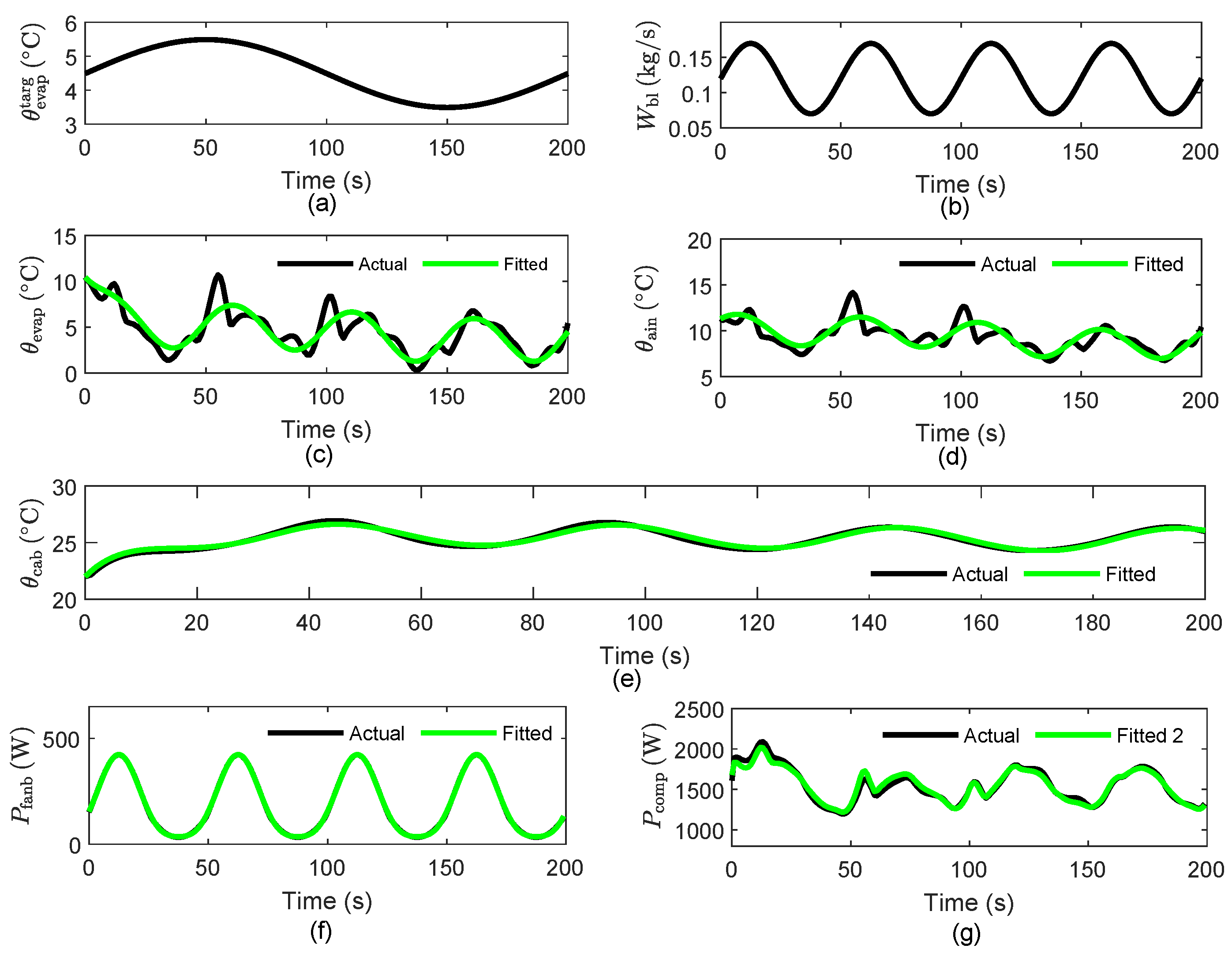
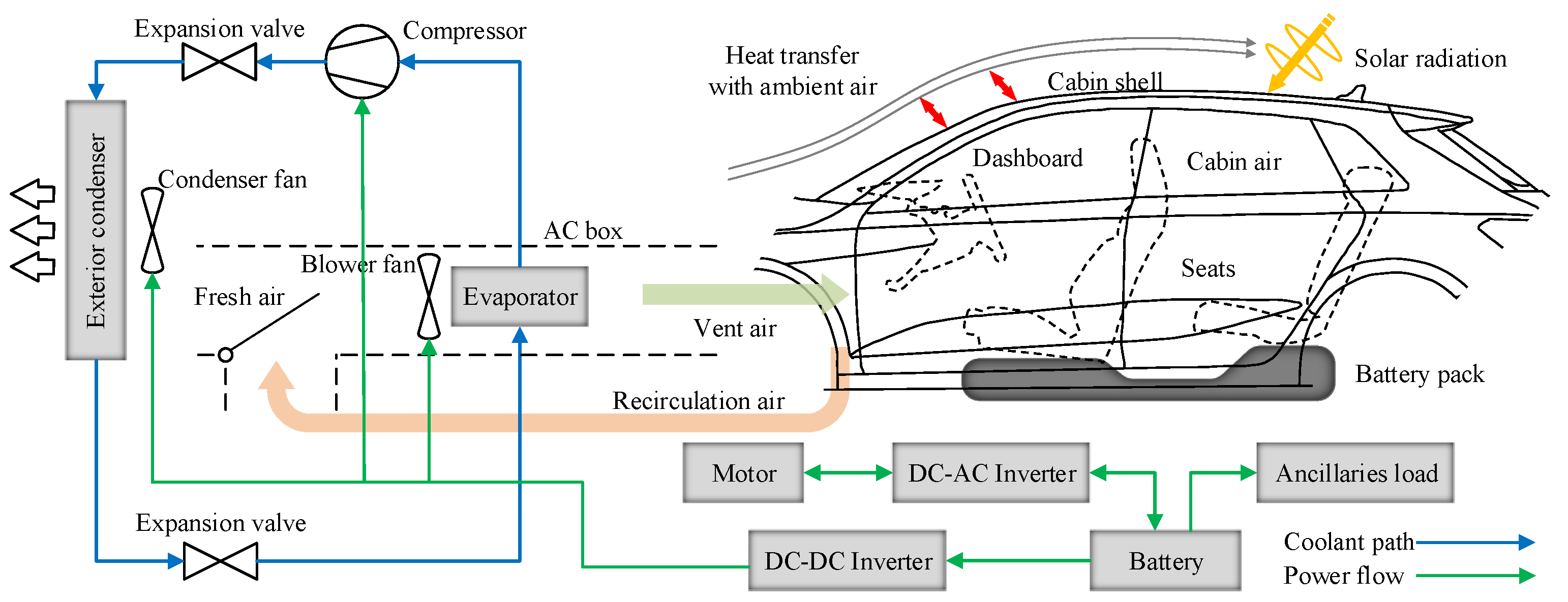
Focusing on Nissan Leaf 2013, which is the prototype vehicle for this study, a benchmark study, along with elaborate experimental measurements, was carried out by Oak Ridge National Laboratory [34]. Based on the experimental data in [34], the power consumption of the entire propulsion system (motor and inverter) $P_{\mathrm{prop}}$ is regarded as a nonlinear function of the motor torque $T_{\mathrm{m}}$ and rotational speed ${\omega }_{\mathrm{m}}$. An interpolation polynomial is chosen to fit the original data

$$P_{\mathrm{prop}}({\omega }_{\mathrm{m}},T_{\mathrm{m}})=p_1+p_2{\omega }_{\mathrm{m}}+p_3{T}_{\mathrm{m}}+p_4{\omega }_{\mathrm{m}}^2+p_5{\omega }_{\mathrm{m}}{T}_{\mathrm{m}}+p_6{T}_{\mathrm{m}}^2,$$

(7)

where the coefficients $p_1$, $p_2$, $p_3$, $p_4$, $p_5$, and $p_6$ are $233.7$, $1.084$, $2.869$, $1.485\times {10}^{-3}$, $0.9972$, and $0.1165$, respectively. The polynomial order is determined by trial and error according to the measured operation data. As demonstrated in Figure 3a, a good fit can be obtained using a second-order polynomial in both ${\omega }_{\mathrm{m}}$ and $T_{\mathrm{m}}$. The bounds on $T_{\mathrm{m}}$ are illustrated in Figure 3b. To remove the need for interpolation, a piecewise nonlinear approximation is implemented on the original bounds, as depicted by the green lines in Figure 3b. A detailed description can be found in [20]. The limits on $T_{\mathrm{m}}$ can be translated as the limits on the longitudinal force (i.e., limits on acceleration)

$$\left\{\begin{array}{c}\max (-c_1,-c_2-c_3{E}_{\mathrm{V}}{\left(k\right)}^{-0.5})\le \frac{rm{a}_{\mathrm{m}}\left(k\right)}{k_{\mathrm{f}}}\hfill \\ \frac{rm{a}_{\mathrm{m}}\left(k\right)}{k_{\mathrm{f}}}\le \min (c_1,c_2+c_3{E}_{\mathrm{V}}{\left(k\right)}^{-0.5}),\hfill \end{array}\right.$$

(8)

where the coefficients $c_1$, $c_2$, and $c_3$ are 280, $-160.9$, and 7381, respectively. Here, ${\omega }_{\mathrm{m}}$ has been expressed as a function of $E_{\mathrm{V}}$.

2.3. AC System

A high-fidelity AC system was established based on CoolSim, which is an open-source modeling environment available from the National Renewable Energy Lab (NREL); the modeling details can be found in [35]. This AC model was validated on experimental data in [36]. To reduce the control complexity, in this study, we perform a system-level analysis for which a simplified control model is more adequate, e.g., the model proposed in [26]. The discrete-time AC model is described as

$$\begin{array}{cc}\hfill & {\theta }_{\mathrm{cab}}(k+1)={\tilde{f}}_{{\theta }_{\mathrm{cab}},t}={\theta }_{\mathrm{cab}}\left(k\right)+{\xi }_1({\theta }_{\mathrm{int}}\left(k\right)-{\theta }_{\mathrm{cab}}\left(k\right))\hfill \\ & +{\xi }_2({\theta }_{\mathrm{shell}}\left(k\right)-{\theta }_{\mathrm{cab}}\left(k\right))+{\xi }_3{W}_{\mathrm{bl}}\left(k\right)({\theta }_{\mathrm{ain}}({\theta }_{\mathrm{evap}},{\theta }_{\mathrm{cab}})-{\theta }_{\mathrm{cab}}\left(k\right))+{\xi }_4\hfill \end{array}$$

(9)

$$\begin{array}{cc}\hfill & {\theta }_{\mathrm{evap}}(k+1)={\tilde{f}}_{{\theta }_{\mathrm{evap}},t}={\theta }_{\mathrm{evap}}\left(k\right)+{\xi }_5({\theta }_{\mathrm{evap}}\left(k\right)-{\theta }_{\mathrm{evap}}^{\mathrm{targ}}\left(k\right))\hfill \\ & +{\xi }_6{W}_{\mathrm{bl}}\left(k\right)({\theta }_{\mathrm{evap}}\left(k\right)-{\theta }_{\mathrm{amb}}\left(k\right))+{\xi }_7\Delta W_{\mathrm{bl}}\left(k\right)({\theta }_{\mathrm{evap}}\left(k\right)-{\theta }_{\mathrm{amb}}\left(k\right))+{\xi }_8\hfill \end{array}$$

(10)

$${\theta }_{\mathrm{ain}}({\theta }_{\mathrm{evap}},{\theta }_{\mathrm{cab}})={\xi }_9{\theta }_{\mathrm{evap}}\left(k\right)+{\xi }_{10}{\theta }_{\mathrm{cab}}\left(k\right)+{\xi }_{11}$$

(11)

$$W_{\mathrm{bl}}(k+1)={\tilde{f}}_{W_{\mathrm{bl}},t}=W_{\mathrm{bl}}\left(k\right)+\Delta W_{\mathrm{bl}}\left(k\right),$$

(12)

where ${\theta }_{\mathrm{cab}}$, ${\theta }_{\mathrm{int}}$, ${\theta }_{\mathrm{shell}}$, ${\theta }_{\mathrm{ain}}$, ${\theta }_{\mathrm{evap}}$, and ${\theta }_{\mathrm{evap}}^{\mathrm{targ}}$ represent the temperature (in $°\mathrm{C}$) of the cabin air, cabin interior, cabin shell, cabin inlet air, evaporator wall, and evaporator wall temperature target, respectively. In Equation (12), $W_{\mathrm{bl}}$ and $\Delta W_{\mathrm{bl}}$ are the blower air flow rate and its increment (in kg/s). The proposed AC model possesses the following characteristics:

• The models given by Equations (9) and (10) are nonlinear due to the bilinear terms in them.
• The variable ${\theta }_{\mathrm{ain}}$ in Equation (9) is just an intermediate or auxiliary variable and not a state variable. It can be directly obtained from Equation (11).
• The temperatures ${\theta }_{\mathrm{int}}$ and ${\theta }_{\mathrm{shell}}$ are dynamic but they change slowly and have little impact on the integration of the system. Hence, they are considered as the input parameters.

In summary, this simplified AC model has three states, ${\theta }_{\mathrm{cab}}$, ${\theta }_{\mathrm{evap}}$, and $W_{\mathrm{bl}}$, and two control inputs, ${\theta }_{\mathrm{evap}}^{\mathrm{targ}}$ and $\Delta W_{\mathrm{bl}}$. Notice that the thermal dynamics are derived from time, which is indicated by the subscript t in the functions ${\tilde{f}}_{{\theta }_{\mathrm{cab}},t}$, ${\tilde{f}}_{{\theta }_{\mathrm{evap}},t}$, and ${\tilde{f}}_{W_{\mathrm{bl}},t}$.

The condenser fan, blower fan, and compressor constitute the primary energy consumers of the AC system. In this work, the power to drive the condenser fan, denoted as $P_{\mathrm{fanc}}$, is set (unchanged) to 233 W [35]. To estimate the blower fan power $P_{\mathrm{fanb}}$, a regression model is directly applied [24]. The compressor power $P_{\mathrm{comp}}$ is usually determined by a simple model involving the difference in energy between the ambient air and cabin inlet air [37]. Based on the test data in CoolSim, $P_{\mathrm{comp}}$ and $P_{\mathrm{fanb}}$ are expressed as

$$P_{\mathrm{comp}}\left(·\right)=\frac{c_{\mathrm{air}}}{\mathrm{COP}}{\beta }_1{W}_{\mathrm{bl}}\left(k\right)({\theta }_{\mathrm{amb}}\left(k\right)-{\theta }_{\mathrm{ain}}\left(·\right))$$

(13)

$$P_{\mathrm{fanb}}\left(W_{\mathrm{bl}}\right)={\beta }_2{W}_{\mathrm{bl}}^2\left(k\right)+{\beta }_3{W}_{\mathrm{bl}}\left(k\right)+{\beta }_4,$$

(14)

where $c_{\mathrm{air}}=1008 \mathrm{J}/\mathrm{kgK}$ is the specific heat capacity of air at constant pressure, COP is the coefficient of performance of the cooling process, ${\theta }_{\mathrm{amb}}$ is the ambient temperature, and $\left(·\right)$ is used as a compact notation for a function of multiple variables. Note that Equation (13) is defined for fresh-air flow, and ${\theta }_{\mathrm{amb}}$ in Equation (13) should be replaced by ${\theta }_{\mathrm{cab}}$ if the cabin air is recirculated.

The unknown parameters in Equations (9)–(14) are identified by collecting the responses of the high-fidelity CoolSim model under different random inputs [24] every 1 s. Figure 4 provides the validation results of the control-oriented AC model, where the first two plots are the sinusoidal inputs to the AC system. Figure 4c–e show the outputs of both the control-oriented model and high-fidelity model.

In comparison to the actual results from the high-fidelity model in CoolSim, the control-oriented AC model shows good accuracy in capturing the trends in the AC system outputs. Additionally, Figure 4f,g show the comparison between the actual AC power in CoolSim and the estimated AC power using Equations (13) and (14). The figure shows that the two sets of data are very close.

2.4. Battery System

The Li-ion battery is modeled by an equivalent circuit model

$$P_{\mathrm{bat}}\left(·\right)=U_{\mathrm{oc}}{I}_{\mathrm{bat}}-I_{\mathrm{bat}}^2{R}_{\mathrm{bat}}=P_{\mathrm{prop}}\left(·\right)+P_{\mathrm{comp}}\left(·\right)+P_{\mathrm{fanb}}\left(W_{\mathrm{bl}}\right)+P_{\mathrm{fanc}},$$

(15)

where $P_{\mathrm{bat}}$ is the power at the battery terminals, $I_{\mathrm{bat}}$ is the current (positive during discharge, negative during charge), $U_{\mathrm{oc}}$ is the open-circuit voltage, and $R_{\mathrm{bat}}$ is the equivalent internal resistance [19,31].

By solving Equation (15), $I_{\mathrm{bat}}$ can be expressed as

$$I_{\mathrm{bat}}\left(·\right)=\frac{U_{\mathrm{oc}}-\sqrt{U_{\mathrm{oc}}^2-4P_{\mathrm{bat}}\left(·\right)R_{\mathrm{bat}}}}{2R_{\mathrm{bat}}}.$$

(16)

The power consumption of the battery at each instant is calculated as the product $U_{\mathrm{oc}}{I}_{\mathrm{bat}}\left(·\right)$.

3. MPC Method and Formulation

In this section, the MPC method is applied to the integrated OCP as described above, and two different MPC problem formulations are described. We first propose a joint optimization-based MPC method in which the objective is to minimize battery energy loss while maintaining cabin-cooling comfort. Then, a co-optimization-based MPC method is presented in which speed planning on hilly roads and cabin-cooling management are treated successively.

3.1. Joint Optimization-Based MPC Method

Although the AC system and propulsion system are two independent systems, their stress on the battery is applied simultaneously. Hence, a general idea is to formulate a joint optimization-based MPC (joint MPC) problem to explore the potential for saving energy.

For each sampling interval, the objective is to minimize the energy costs by integrating the battery power

$$J\left(·\right)=U_{\mathrm{oc}}{I}_{\mathrm{bat}}(x,u,w)\frac{\Delta s}{\sqrt{2E_{\mathrm{V}}}},$$

(17)

where $\Delta s/\sqrt{2E_{\mathrm{V}}}$ denotes the passing time per sampling interval. Here, x, u, and w are the states, control inputs, and predicted disturbances, which are described in more detail below.

Besides minimizing energy costs, the MPC is required to keep states within bounds. Some of these bounds, including the speed and cabin temperature limits, are allowed to be violated for a short period. This is modeled by relaxing the state constraints as

$$\frac{v_{\min }{\left(k\right|i)}^2}{2}\le E_{\mathrm{v}}\left(k\right|i)+{\delta }_{E_{\mathrm{v}}}\left(k\right|i)\le \frac{v_{\max }{\left(k\right|i)}^2}{2}$$

(18)

$${\theta }_{{\mathrm{cab}}_{\min }}\le {\theta }_{\mathrm{cab}}\left(k\right|i)+{\delta }_{{\theta }_{\mathrm{cab}}}\left(k\right|i)\le {\theta }_{{\mathrm{cab}}_{\max }},$$

(19)

where $v_{\min }\left(k\right|i)$ and $v_{\max }\left(k\right|i)$ are the minimum and maximum allowable speeds along the prediction horizon and ${\delta }_{E_{\mathrm{v}}}$ and ${\delta }_{{\theta }_{\mathrm{cab}}}$ are slack variables. The severity of the constraint violation is regulated by penalizing the slack variables within the objective function.

To better regulate the cabin temperature, an additional constraint is imposed to maintain the average cabin temperature ${\theta }_{\mathrm{cab}}^{\mathrm{avg}}$ at the desired target temperature ${\theta }_{\mathrm{cab}}^{\mathrm{targ}}$ within the prediction horizon. This requires introducing a new state

$${\theta }_{\mathrm{cab}}^{\mathrm{avg}}(k+1)={\tilde{f}}_{{\theta }_{\mathrm{cab}}^{\mathrm{avg}},t}={\theta }_{\mathrm{cab}}^{\mathrm{avg}}\left(k\right)+\frac{\Delta t{\theta }_{\mathrm{cab}}\left(k\right)}{t_{\mathrm{des}}},$$

(20)

where $t_{\mathrm{des}}$ is the desired driving time along the prediction horizon and ${\theta }_{\mathrm{cab}}^{\mathrm{avg}}\left(0\right)=0$. The cooling demand can be strictly met by constraining the average cabin temperature at the end of the horizon to

$${\theta }_{\mathrm{cab}}^{\mathrm{avg}}\left(N\right)+{\delta }_{{\theta }_{\mathrm{cab}}^{\mathrm{avg}}}={\theta }_{\mathrm{cab}}^{\mathrm{targ}},$$

(21)

where N is the number of samples along the horizon. During the first few MPC updates, the cooling system may not be powerful enough to keep the average temperature at the target value. Hence, Equation (21) is relaxed by the slack variable ${\delta }_{{\theta }_{\mathrm{cab}}^{\mathrm{avg}}}$, which is a scalar value that will also be penalized in the objective function.

In principle, it is not necessary to introduce the new state ${\theta }_{\mathrm{cab}}^{\mathrm{avg}}$, as the cabin temperature can also be regulated by a penalizing deviation from ${\theta }_{\mathrm{cab}}^{\mathrm{targ}}$ within the objective function. However, this would require the tuning of an additional penalty for the temperature deviation, which is avoided by the formulation with the new state.

The vectors of the states, control inputs, and predicted disturbances in the joint MPC can be summarized as

$$\left\{\begin{array}{c}x={\left[\begin{array}{cccccc}{E}_{\mathrm{V}}& t& {\theta }_{\mathrm{cab}}& {\theta }_{\mathrm{evap}}& W_{\mathrm{bl}}& {\theta }_{\mathrm{cab}}^{\mathrm{avg}}\end{array}\right]}^{\top }\hfill \\ u={\left[\begin{array}{ccc}{a}_{\mathrm{m}}& {\theta }_{\mathrm{evap}}^{\mathrm{targ}}& \Delta W_{\mathrm{bl}}\end{array}\right]}^{\top }\hfill \\ w={\left[\begin{array}{cccc}\alpha & {\theta }_{\mathrm{amb}}& {\theta }_{\mathrm{int}}& {\theta }_{\mathrm{shell}}\end{array}\right]}^{\top },\hfill \end{array}\right.$$

(22)

respectively. Combining Equations (2)–(4), Equations (9)–(12), and (20), the system dynamics can be written as

$${\tilde{f}}_s={\left[\begin{array}{cccccc}{\tilde{f}}_{E_{\mathrm{V}},s}& {\tilde{f}}_{t,s}& {\tilde{f}}_{{\theta }_{\mathrm{cab}},s}& {\tilde{f}}_{{\theta }_{\mathrm{evap}},s}& {\tilde{f}}_{W_{\mathrm{bl}},s}& {\tilde{f}}_{{\theta }_{\mathrm{cab}}^{\mathrm{avg}},s}\end{array}\right]}^{\top },$$

(23)

where ${\tilde{f}}_{{\theta }_{\mathrm{cab}},s}$, ${\tilde{f}}_{{\theta }_{\mathrm{evap}},s}$, ${\tilde{f}}_{W_{\mathrm{bl}},s}$, and ${\tilde{f}}_{{\theta }_{\mathrm{cab}}^{\mathrm{avg}},s}$ can be easily obtained from ${\tilde{f}}_{{\theta }_{\mathrm{cab}},t}$, ${\tilde{f}}_{{\theta }_{\mathrm{evap}},t}$, ${\tilde{f}}_{W_{\mathrm{bl}},t}$, and ${\tilde{f}}_{{\theta }_{\mathrm{cab}}^{\mathrm{avg}},t}$ by applying a simple conversion, as follows. For any of the four thermal states, ${\theta }_{\mathrm{cab}}$, ${\theta }_{\mathrm{evap}}$, $W_{\mathrm{bl}}$, and ${\theta }_{\mathrm{cab}}^{\mathrm{avg}}$, their discrete dynamics in both the time and space domains can be written using first-order discretization as

$$\left\{\begin{array}{c}x(k+1)=x\left(k\right)+\Delta t{f}_t={\tilde{f}}_{x,t}\hfill \\ x(k+1)=x\left(k\right)+\frac{\Delta s}{\sqrt{2E_{\mathrm{V}}}}{f}_t={\tilde{f}}_{x,s},\hfill \end{array}\right.$$

(24)

respectively. Eliminating $f_t$, the dynamics in the space domain ${\tilde{f}}_{x,s}$ are rewritten as

$${\tilde{f}}_{x,s}=x\left(k\right)\left(1-\frac{\Delta s}{\sqrt{2E_{\mathrm{V}}}\Delta t}\right)+\frac{\Delta s{\tilde{f}}_{x,t}}{\sqrt{2E_{\mathrm{V}}}\Delta t}.$$

(25)

In its more general form, the joint MPC in the discrete space with the prediction made at the time instant i is defined as

$$\begin{array}{cc}\hfill & \min \sum _{k=1}^N\left(J(x,u,w)+W({\delta }_{E_{\mathrm{v}}},{\delta }_{{\theta }_{\mathrm{cab}}})\right)+{\rho }_{{\theta }_{\mathrm{cab}}^{\mathrm{avg}}}{\delta }_{{\theta }_{\mathrm{cab}}^{\mathrm{avg}}}^2\left(i\right)\hfill \\ \hfill & \mathrm{subject}\mathrm{to}\hfill \end{array}$$

(26a)

$$\begin{array}{cc}\hfill & x(k+1|i)={\tilde{f}}_s(x\left(k\right|i),u\left(k\right|i),w\left(k\right|i))\hfill \end{array}$$

(26b)

$$\begin{array}{cc}\hfill & x\left(k\right|i)\in [x_{\min }\left(k\right|i),x_{\max }\left(k\right|i)]\hfill \end{array}$$

(26c)

$$\begin{array}{cc}\hfill & u\left(k\right|i)\in [u_{\min }\left(i\right),u_{\max }\left(i\right)]\hfill \end{array}$$

(26d)

$$\begin{array}{cc}\hfill & g(x,u,w)\le 0\hfill \end{array}$$

(26e)

$$\begin{array}{cc}\hfill & x\left(0\right|i)=x(i),\hfill \end{array}$$

(26f)

$$\begin{array}{cc}\hfill & x\left(N_1\right|i)\in \mathcal{X}\left(i\right)\hfill \end{array}$$

(26g)

where k is the discrete index for the sample along the horizon. The penalties of the slack variables

$$W({\delta }_{E_{\mathrm{v}}},{\delta }_{{\theta }_{\mathrm{cab}}})={\rho }_{E_{\mathrm{v}}}{\delta }_{E_{\mathrm{v}}}^2\left(k\right|i)+{\rho }_{{\theta }_{\mathrm{cab}}}{\delta }_{{\theta }_{\mathrm{cab}}}^2\left(k\right|i)$$

(27)

and ${\rho }_{{\theta }_{\mathrm{cab}}^{\mathrm{avg}}}{\delta }_{{\theta }_{\mathrm{cab}}^{\mathrm{avg}}}^2\left(i\right)$ are added to the objective function Equation (26a). The penalty factors ${\rho }_{E_{\mathrm{v}}}$, ${\rho }_{{\theta }_{\mathrm{cab}}}$, and ${\rho }_{{\theta }_{\mathrm{cab}}^{\mathrm{avg}}}$ are generally set to large values. The constraints of all the state and control variables are defined by Equations (26b)–(26d) according to the system operating requirements. Equation (26e) collects all inequality constraints. The initial state values can be found in Equation (26f), and a target set for all the final state values is imposed by Equation (26g). From the disturbance vector, the road slope $\alpha \left(k\right|i)$ is assumed to be known along the prediction horizon, whereas the remaining disturbances, ${\theta }_{\mathrm{int}}\left(i\right)$ and ${\theta }_{\mathrm{shell}}\left(i\right)$, are assumed constant along the prediction horizon but may change value at different MPC updates, invoked at sample i.

The vector function in Equation (26e) includes three sets of inequality constraints:

• The speed and cabin temperature limits in Equations (18) and (19).
• Limits on the motor torque in Equation (8).
• Vehicle acceleration limits $a_{\min }$ and $a_{\max }$ imposed to reduce driving discomfort,

  $$a_{\min }\le f_{E_{\mathrm{V}},s}\left(k\right|i)\le a_{\max },$$

  (28)

  where the vehicle acceleration equals $f_{E_{\mathrm{V}},s}$, as shown in Equation (2).

The target set $\mathcal{X}\left(i\right)$ in Equation (26g) contains three items called by the optimization mission:

• The passing time over the prediction horizon N, which should adhere to a specified value

  $$t\left(N\right|i)-t\left(0\right|i)\le t_{\mathrm{des}}\left(i\right),$$

  (29)

  where $t_{\mathrm{des}}$ is the desired passing time and is computed by

  $$t_{\mathrm{des}}\left(i\right)=\sum _{k=1}^N\frac{2\Delta s}{v_{\min }\left(k\right|i)+v_{\max }\left(k\right|i)}.$$

  (30)
• The target speed, as the vehicle is expected to end the horizon with the average or greater speed. This requires

  $$\begin{array}{c}\hfill E_{\mathrm{V}}\left(N\right|i)\ge \frac{1}{2}{\left(\frac{v_{\min }\left(N\right|i)+v_{\max }\left(N\right|i)}{2}\right)}^2={(v_{\min }\left(N\right|i)+v_{\max }\left(N\right|i))}^2/8.\end{array}$$

  (31)
• The target average cabin temperature in Equation (21).

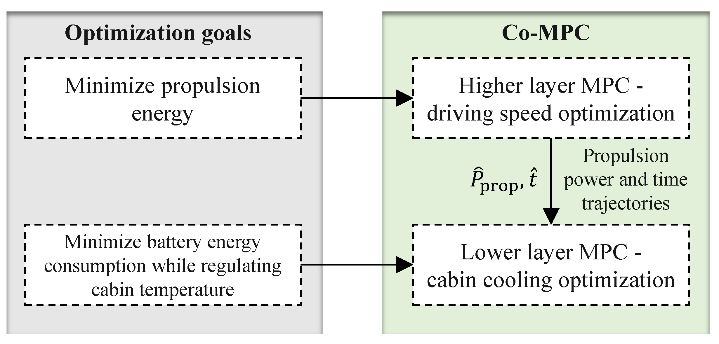
3.2. Co-Optimization-Based MPC Method

A sub-optimal solution to the joint optimization problem is a co-optimization-based MPC (co-MPC). The control structure of the co-MPC is shown in Figure 5. It can be seen that the co-MPC is a two-layer approach, where two MPCs are customized for the driving speed optimization and cabin-cooling optimization, respectively. The higher-layer MPC (HMPC) computes the propulsion power and time trajectories (${\widehat{P}}_{\mathrm{prop}}$, $\widehat{t}$) to the end of the horizon. Then, the lower-layer MPC (LMPC) uses these trajectories to compute the control inputs to the AC system.

Aiming to minimize the net propulsion energy, the HMPC is defined in the discrete space to directly utilize the road information predicted at instant i,

$$\begin{array}{cc}\hfill & \min \sum _{k=1}^{N_{\mathrm{h}}}\left(P_{\mathrm{prop}}\frac{\Delta s}{\sqrt{2E_{\mathrm{V}}/m}}+{\rho }_{E_{\mathrm{v}}}{\delta }_{E_{\mathrm{v}}}^2\right)\hfill \\ \hfill & \mathrm{subject}\mathrm{to}\hfill \end{array}$$

(32a)

$$\begin{array}{cc}\hfill & x_{\mathrm{h}}(k+1|i)={\tilde{f}}_{s,\mathrm{h}}(x_{\mathrm{h}}\left(k\right|i),u_{\mathrm{h}}\left(k\right|i),w_{\mathrm{h}}\left(k\right|i))\hfill \end{array}$$

(32b)

$$\begin{array}{cc}\hfill & x_{\mathrm{h}}\left(k\right|i)\in [x_{\mathrm{h},\min }\left(k\right|i),x_{\mathrm{h},\max }\left(k\right|i)]\hfill \end{array}$$

(32c)

$$\begin{array}{cc}\hfill & u_{\mathrm{h}}\left(k\right|i)\in [u_{\mathrm{h},\min }\left(i\right),u_{\mathrm{h},\max }\left(i\right)]\hfill \end{array}$$

(32d)

$$\begin{array}{cc}\hfill & g_{\mathrm{h}}(x_{\mathrm{h}},u_{\mathrm{h}},w_{\mathrm{h}})\le 0\hfill \end{array}$$

(32e)

$$\begin{array}{cc}\hfill & x_{\mathrm{h}}\left(0\right|i)=x_{\mathrm{h}}\left(i\right),\hfill \end{array}$$

(32f)

$$\begin{array}{cc}\hfill & x_{\mathrm{h}}\left(N_{\mathrm{h}}\right|i)\in {\mathcal{X}}_{\mathrm{h}}\left(i\right)\hfill \end{array}$$

(32g)

where $N_{\mathrm{h}}$ is the prediction horizon. In this problem, the state, control, and auxiliary variables are set as

$$x_{\mathrm{h}}={\left[E_{\mathrm{V}}t\right]}^{\mathrm{T}},u_{\mathrm{h}}=\left[a_{\mathrm{m}}\right],w_{\mathrm{h}}=\left[\alpha \right],$$

(33)

and ${\tilde{f}}_{s,\mathrm{h}}={\left[{\tilde{f}}_{E_{\mathrm{V}},s}{\tilde{f}}_{t,s}\right]}^{\mathrm{T}}$ is the state dynamics vector. The constraints of all system variables and inequality constraints, along with the initial state values and final state targets, are indicated by Equations (32c)–(32g). Details can be found in Section 3.1.

The LMPC is designed, as seen in Figure 5, to minimize battery energy consumption while regulating cabin temperature similarly to the joint MPC. However, although the joint MPC is implemented in the space domain, the LMPC is implemented in the time domain, as the prediction of the speed trajectory is now available from the HMPC. Taking $N_{\mathrm{l}}$ and $\Delta t$ as the prediction horizon and the sampling interval, the LMPC in the discrete time with disturbance ${\widehat{P}}_{\mathrm{prop}}$ predicted at the time instant i is defined as

$$\begin{array}{cc}\hfill & \min \sum _{k=1}^{N_{\mathrm{l}}}\left(U_{\mathrm{oc}}{I}_{\mathrm{bat}}(x_{\mathrm{l}},u_{\mathrm{l}},w_{\mathrm{l}})\Delta t+{\rho }_{{\theta }_{\mathrm{cab}}}{\delta }_{{\theta }_{\mathrm{cab}}}^2\right)+{\rho }_{{\theta }_{\mathrm{cab}}^{\mathrm{avg}}}{\delta }_{{\theta }_{\mathrm{cab}}^{\mathrm{avg}}}^2\left(i\right)\hfill \\ \hfill & \mathrm{subject}\mathrm{to}\hfill \end{array}$$

(34a)

$$\begin{array}{cc}\hfill & x_{\mathrm{l}}(k+1|i)={\tilde{f}}_{t,\mathrm{l}}(x_{\mathrm{l}}\left(k\right|i),u_{\mathrm{l}}\left(k\right|i),w_{\mathrm{l}}\left(k\right|i))\hfill \end{array}$$

(34b)

$$\begin{array}{cc}\hfill & x_{\mathrm{l}}\left(k\right|i)\in [x_{\mathrm{l},\min }\left(k\right|i),x_{\mathrm{l},\max }\left(k\right|i)]\hfill \end{array}$$

(34c)

$$\begin{array}{cc}\hfill & u_{\mathrm{l}}\left(k\right|i)\in [u_{\mathrm{l},\min }\left(i\right),u_{\mathrm{l},\max }\left(i\right)]\hfill \end{array}$$

(34d)

$$\begin{array}{cc}\hfill & x_{\mathrm{l}}\left(0\right|i)=x_{\mathrm{l}}\left(i\right),\hfill \end{array}$$

(34e)

$$\begin{array}{cc}\hfill & {\theta }_{\mathrm{cab}}^{\mathrm{avg}}\left(N_{\mathrm{l}}\right)={\theta }_{\mathrm{cab}}^{\mathrm{targ}}\hfill \end{array}$$

(34f)

where the index k indicates the current travel time of the vehicle. The state, control, and auxiliary variables are set as

$$\left\{\begin{array}{c}{x}_{\mathrm{l}}={\left[{\theta }_{\mathrm{cab}}{\theta }_{\mathrm{evap}}{W}_{\mathrm{bl}}{\theta }_{\mathrm{cab}}^{\mathrm{avg}}\right]}^{\mathrm{T}}\hfill \\ u_{\mathrm{l}}={[{\theta }_{\mathrm{evap}}^{\mathrm{targ}}\Delta W_{\mathrm{bl}}]}^{\mathrm{T}}\hfill \\ w_{\mathrm{l}}={\left[P_{\mathrm{prop}}{\theta }_{\mathrm{amb}}{\theta }_{\mathrm{int}}{\theta }_{\mathrm{shell}}\right]}^{\mathrm{T}},\hfill \end{array}\right.$$

(35)

and ${\tilde{f}}_{t,\mathrm{l}}={\left[{\tilde{f}}_{{\theta }_{\mathrm{cab}},t}{\tilde{f}}_{{\theta }_{\mathrm{evap}},t}{\tilde{f}}_{W_{\mathrm{bl}},t}{\tilde{f}}_{{\theta }_{\mathrm{cab}}^{\mathrm{avg}},t}\right]}^{\mathrm{T}}$ is the state dynamics vector. It should be noted that $t_{\mathrm{des}}$ used in Equation (20) has been replaced with $N_{\mathrm{l}}\Delta t$. The constraints of the state and control variables, as well as the initial states and final state target, are indicated by Equations (34c)–(34f). Please see Section 3.1 for more details.

4. Case Studies

The established MPCs were first verified using an urban expressway segment of a length of 20 km located between Xuanwu Nanjing and Jurong Zhenjiang in China. The altitude information was taken from the Google Elevation API. In this study, we assumed that there was no leading vehicle on the road, which meant that the ego vehicle could freely change its speed within the given limits. The upper speed limit was set to 70 km/h according to the legal limit, whereas the lower limit was set to 50 km/h to avoid blocking traffic. Meanwhile, ${\theta }_{\mathrm{amb}}$ and ${\theta }_{\mathrm{cab}}^{\mathrm{targ}}$ were set at 30 $°\mathrm{C}$ and 24 $°\mathrm{C}$ to imitate a summer cooling scenario. Other parameters used in the constraints on the state variables and control inputs are given as

$$\left\{\begin{array}{c}{\theta }_{\mathrm{cab}}\in [23.5°\mathrm{C},24.5°\mathrm{C}]\hfill \\ {\theta }_{\mathrm{evap}}\in [0°\mathrm{C},12°\mathrm{C}]\hfill \\ W_{\mathrm{bl}}\in [0.02 \mathrm{k}\mathrm{g}/\mathrm{s},0.18 \mathrm{k}\mathrm{g}/\mathrm{s}]\hfill \\ {\theta }_{\mathrm{evap}}^{\mathrm{targ}}\in [3°\mathrm{C},10°\mathrm{C}]\hfill \\ \Delta W_{\mathrm{bl}}\in [-0.05 \mathrm{k}\mathrm{g}/\mathrm{s},0.05 \mathrm{k}\mathrm{g}/\mathrm{s}]\hfill \\ a\in [-1.5 \mathrm{m}/{\mathrm{s}}^2,1.5 \mathrm{m}/{\mathrm{s}}^2].\hfill \end{array}\right.$$

(36)

4.1. Parameters and Numerical Solver

The parameters of the EV and AC models are listed in

Table 1. Parameters of the EV and AC models.

Parameter	Value
Vehicle mass m	1521 kg
Aerodynamic drag coefficient $C_{\mathrm{D}}$	$0.32$
Vehicle front area $A_{\mathrm{f}}$	$2.277$ m2
Rolling resistance coefficient f	0.015
Air density $\rho$	$1.2$ kg/m3
Gravitational acceleration g	$9.81$ m/s2
Wheel radius r	$0.316$ m
Battery normal voltage $U_{\mathrm{oc}}$	365 V
Battery pack resistance $R_{\mathrm{bat}}$	$0.11$$\Omega$
Specific heat capacity of air $c_{\mathrm{air}}$	$1008 \mathrm{J}/\mathrm{kgK}$
Coefficient of performance COP	$3.5$
AC parameter ${\xi }_{\mathrm{j}}(j=1,2,\dots ,11)$	[0.0699,0.0298,0.3566,−0.2961,−0.0845,−0.1004,
	−1.5820,−0.3278,0.7205,0.6874,−11.3561]
AC parameter ${\beta }_{\mathrm{j}}(j=1,2,3,4)$	[1.51,26293,−2437,71]

, whereas

Table 2. Parameters of the joint MPC and co-MPC.

	Parameter	Value
Joint MPC	Sampling interval $\Delta s$	20 m
	Prediction/control horizon N	50
Co-MPC	Sampling interval $\Delta s$, $\Delta t$	20 m, 1 s
	Prediction/control horizon $N_{\mathrm{h}}$, $N_{\mathrm{l}}$	50, 60

lists the design parameters of the joint MPC and co-MPC. As indicated in Table 1, the control horizon was identical to the prediction horizon. The settings were chosen to balance the control performance and computational cost. The software CasADi with the interior-point optimization solver (IPOPT) was selected to solve the established MPCs [38]. The simulations were conducted on a desktop computer (Intel i7-11700 CPU with 2.5 GHz and 16 GB RAM) using MATLAB 2019a.

4.2. Reference Methods

Two reference control methods were developed for comparison purposes. The first method employed an ideal constant-speed (CS) strategy, whereas the AC system employed a proportion integral (PI) strategy that is commonly applied to real-life vehicles. The PI strategy regulated the evaporator wall temperature and the blower rate to maintain the desired cabin air temperature. Detailed information about this PI strategy can be found in [39]. The second method adopted the HMPC proposed in Section 3.2 to regulate the driving speed, whereas the AC system was regulated by the PI. The above two reference methods are named CS-PI and HMPC-PI, respectively.

Since the CS and PI were similar to the actual strategies, the CS-PI was considered the baseline for the other methods. The HMPC-PI was used to demonstrate not only the benefits of the speed optimization in comparison with the CS-PI but also the marginal benefits achieved by the integrated optimization in comparison with the proposed joint MPC and co-MPC.

4.3. Simulation Results

The altitude profile of the expressway and the speed trajectories are shown in Figure 6a,b. As observed in the bottom plot, the driving speed was regulated by the road’s speed limit. The HMPC-PI, co-MPC, and joint MPC show qualitatively similar speed trajectories, which, in combination with the altitude profile in the top plot, yield the following features: acceleration before going uphill, deceleration while going uphill, and acceleration while going downhill. However, the variation in the amplitude of the joint MPC is greater than those of the HMPC-PI and co-MPC. The acceleration profiles in Figure 6c also confirm the effectiveness of the acceleration constraint. The jerk profiles shown in Figure 6d are also provided here for a later discussion about driving comfort.

To help clarify the behavior of cabin-cooling management, an LMPC control over a single MPC update is presented before discussing the overall simulation results. In this example, we assumed that the propulsion power over the prediction horizon ${\widehat{P}}_{\mathrm{prop}}$ had been calculated through the HMPC and had a simple form, as shown in Figure 7a. It can be seen in Figure 7b that the cabin air temperature in both recirculation mode and fresh-air mode exhibits similar trends. Initially set at 24 $°\mathrm{C}$, ${\theta }_{\mathrm{cab}}$ was forced to decrease below the desired value. Following this, ${\theta }_{\mathrm{cab}}$ was gradually raised to a high value and finally dropped back to the desired value.

Comparing the results in the two AC modes with and without cabin air recirculation, we find that:

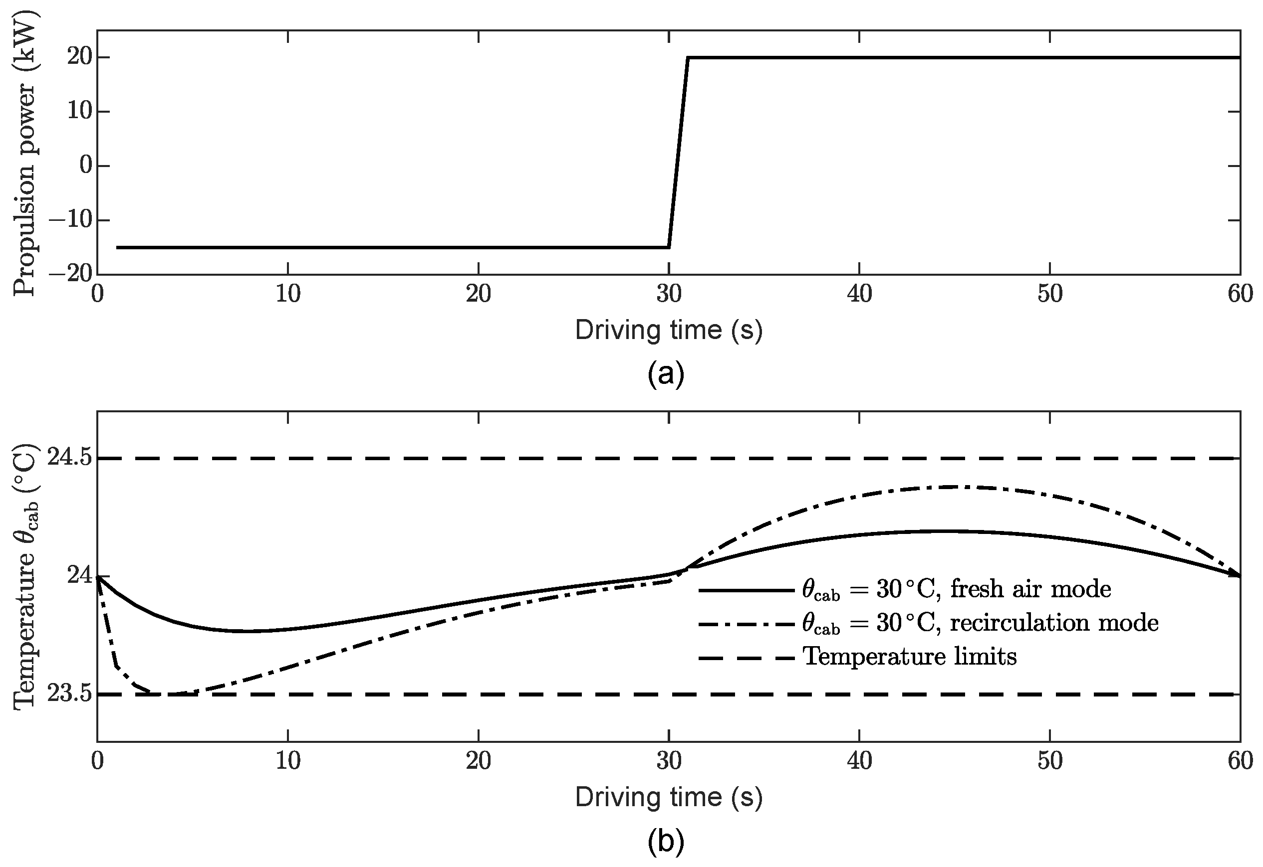
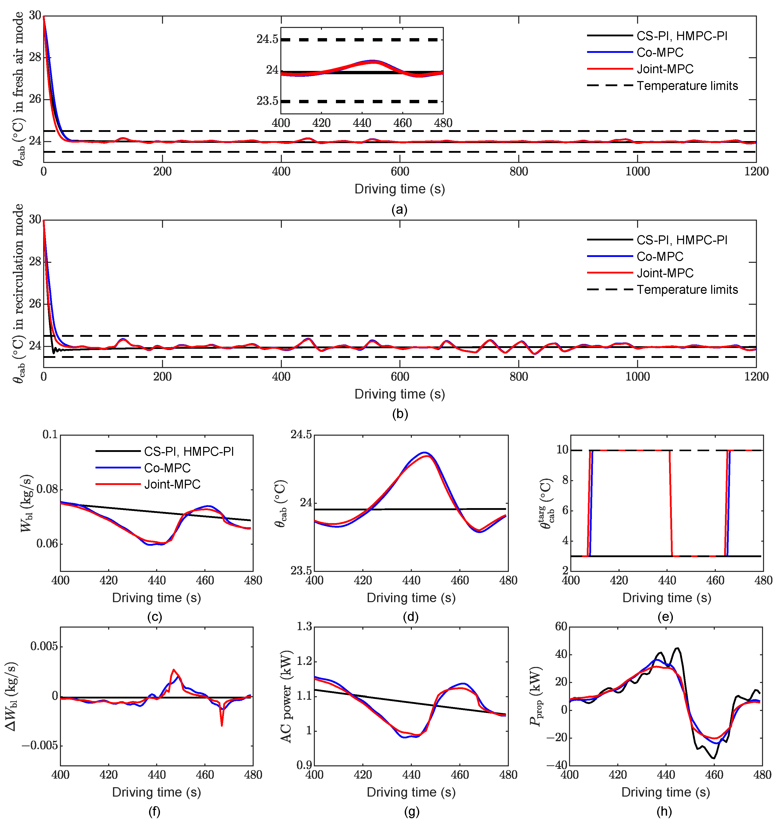
• In fresh-air mode and when the propulsion power is negative, the proposed LMPC does not decrease the cabin temperature too much below the average. This is because the thermal losses increase with the difference between the ambient and cabin temperatures and are much greater than the losses from cycling the energy twice through the battery, i.e., first recuperating the braking energy in the battery, and then using it later to cool down the cabin when the propulsion power is positive. Hence, the thermal buffer in fresh-air mode is much less efficient than the electric buffer.
• In recirculation mode, the LMPC can make greater use of the thermal buffer to reduce energy losses caused by double electricity cycling. During negative propulsion power, the braking energy is used directly by the AC system to cool the cabin until the lower temperature limit is reached, thus reducing the amount of energy recuperated in the battery. During the positive propulsion power, the cabin temperature passively increases due to the influence of the hot ambient temperature, although the battery energy is still needed by the AC system to keep the average temperature at 24 $°\mathrm{C}$. As a result, the thermal buffer exhibits higher efficiency in recirculation mode than in fresh-air mode.

Figure 8a,b show the cabin air temperature trajectories over the entire trip for the two AC modes. In Figure 8a, it can be seen that ${\theta }_{\mathrm{cab}}$ drops rapidly from the initial 30 $°\mathrm{C}$ to around the desired 24 $°\mathrm{C}$ for all methods. During the remaining driving time, the CS-PI and HMPC-PI cause ${\theta }_{\mathrm{cab}}$ to stay nearly constant. On the contrary, both the co-MPC and joint MPC cause ${\theta }_{\mathrm{cab}}$ to change slightly around the desired 24 $°\mathrm{C}$, as shown in the amplified plot in Figure 8a. In Figure 8b, it can be seen that ${\theta }_{\mathrm{cab}}$ initially reaches the same cabin temperature in a shorter period of time due to the fact that the cabin air is recycled to blow the evaporator during recirculation mode. On the other hand, the thermal buffer is better utilized in recirculation mode.

A comparison of the AC system outputs of the different methods during a short period [ 400 s 480 s] is shown in Figure 8c–h. Both the CS-PI and HMPC-PI maintain almost constant cabin air temperatures and blower rates, with only small decreases in the blower rate, as indicated by the black lines in Figure 8c,d. As with the co-MPC and joint MPC, the blower rate displays similar patterns. In contrast, the cabin air temperature shows the opposite trend in the blower rate, as shown by the blue and red lines in Figure 8d. Figure 8e,f present the control inputs to the AC system. As can be seen, the proposed co-MPC and joint MPC allow the evaporator wall temperature target to jump to the high bound, thus reducing the cooling demand. The last two plots in Figure 8 show the AC power and propulsion power, respectively. Based on these power curves and the aforementioned case study of an LPMC update, it can be concluded that the proposed co-MPC and joint MPC demonstrate the same power management approach for AC power: the AC power decreases when the propulsion motor is consuming high power; the AC power increases when the propulsion power is low.

To test the MPC under various road conditions, we included a hilly road between Chengdu and Chongqing in China with a length of 14 km, whose terrain can be seen in Figure 9a. The high and low speed limits were set to 80 km/h and 40 km/h, respectively.

The simulation results for the second case are illustrated in Figure 9, where the results in fresh-air mode are ignored for simplicity. The terrain shown in Figure 9a displays fewer saddles; thus, the regulated speed appears smoother. According to Figure 9b, only the range [47,73] km/h is activated, which implies that maximizing the speed band usage is not always required for optimal speed planning. In terms of the cabin air temperature, the co-MPC and joint MPC produced similar results, as shown in Figure 9c.

5. Performance Evaluation

In this section, the performance of the proposed methods in terms of energy efficiency, thermal comfort, and computation time is discussed.

5.1. Energy Consumption Evaluation

Based on the simulation results of the first case study, the performances of the different methods were summarized and are shown in

Table 3. Performance of the four methods in the first case study.

MPC Method	CS-PI		HMPC-PI		Co-MPC		Joint MPC
	Fresh	Recir	Fresh	Recir	Fresh	Recir	Fresh	Recir
Average speed (km/h)	60.00	60.00	60.02	60.02	60.02	60.02	60.01	60.04
Average ${\theta }_{\mathrm{cab}}$ ($°\mathrm{C}$)	23.97	23.97	23.97	23.98	23.98	23.97	23.94	23.95
Propulsion energy (MJ)	7.969	7.969	7.862	7.862	7.862	7.862	7.856	7.850
AC energy (MJ)	2.891	1.218	2.891	1.218	2.806	1.179	2.800	1.174
Battery energy (MJ)	11.123	9.426	10.940	9.244	10.853	9.203	10.821	9.183

. The first two rows in Table 3 illustrate that the average speed and average cabin temperature of each control method were maintained at around 60 km/h and 24 $°\mathrm{C}$, respectively. Therefore, it is reasonable to compare energy consumption hereafter.

For the first scenario in fresh-air mode, the propulsion energy, AC energy, and battery energy of the CS-PI were $7.969$ MJ, $2.891$ MJ, and $11.123$ MJ, respectively. In recirculation mode, the corresponding values were $7.969$ MJ, $1.218$ MJ, and $9.426$ MJ. Taking these values as the baseline, the energy benefits earned by the other three methods in the two AC modes were determined and are depicted in Figure 10.

It can be seen in Figure 10a that driving speed optimization with HMPC can reduce propulsion energy by 1.34%. Using the cooling management in the co-MPC can enable a 2.94% AC energy reduction compared to the HMPC-PI in fresh-air mode. Hence, the co-MPC finally obtained a 2.43% total reduction in battery energy consumption, which is 0.78% higher than that of the HMPC-PI. As expected, among the three methods, the joint MPC achieved the most savings. For instance, the joint MPC generates 2.72% savings in battery energy loss, which is 1.07% higher than that of the HMPC-PI and 0.29% higher than that of the co-MPC. Such additional 0.29% benefits are understandable since the global solution Equation (26) theoretically allows a larger space for optimization than the co-optimization solutions Equations (32) and (34).

When compared to fresh air mode, the co-MPC and joint MPC achieve greater AC energy savings in recirculation mode, i.e., 4.01% and 4.41%, as listed in Figure 10b. These results are reasonable since the thermal buffer is more effectively utilized in this mode, as previously discussed. The battery energy savings of the three methods were 1.93%, 2.36%, and 2.58%. Thus, compared to the HMPC-PI, the marginal AC benefits achieved by the joint MPC were 0.65%.

Table 4. Performance of the four methods in the second case study.

MPC Method	CS-PI		HMPC-PI		Co-MPC		Joint MPC
	Fresh	Recir	Fresh	Recir	Fresh	Recir	Fresh	Recir
Average speed (km/h)	60.00	60.00	59.98	59.98	59.98	59.98	59.95	59.95
Average ${\theta }_{\mathrm{cab}}$ ($°\mathrm{C}$)	24.00	24.00	24.00	24.00	24.01	24.00	24.01	24.01
Propulsion energy (MJ)	5.022	5.022	4.952	4.952	4.952	4.952	4.924	4.925
AC energy (MJ)	1.620	0.956	1.620	0.956	1.569	0.917	1.566	0.913
Battery energy (MJ)	6.985	6.345	6.915	6.275	6.839	6.204	6.825	6.181

summarizes the performance of the four methods in the second case study and Figure 11 provides the statistical energy benefits obtained from Table 4. As can be seen, the co-MPC yielded a battery energy reduction of 2.09–2.22%, whereas the joint MPC resulted in a reduction of 2.29–2.58%. Compared to the HMPC-PI, the marginal AC benefits achieved by the joint MPC were as large as 1.48%.

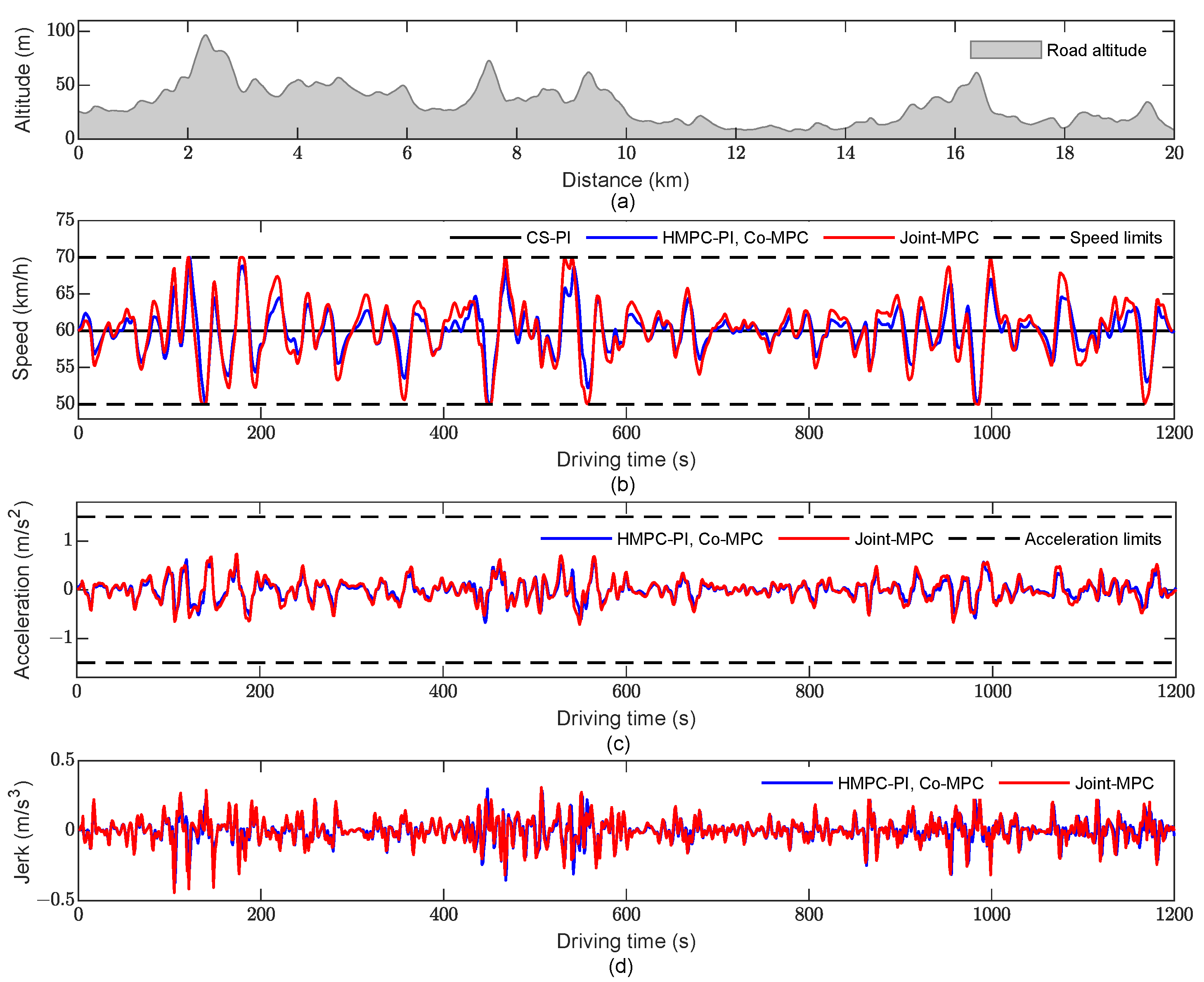
5.2. Driving and Thermal Comfort

We illustrated the acceleration profiles of the different control methods when the AC was running in fresh-air mode in Section 4.3. As shown in Figure 6c, both the co-MPC and joint MPC maintained the vehicle acceleration strictly within [−1.5, 1.5] m/s². In addition, according to Figure 6d, the jerk profiles stabilized at [−0.5, 0.5] m/s³, which should not cause any significant discomfort. We can conclude that the proposed MPCs provide acceptable driving comfort.

Both the average cabin air temperature and the severity of the temperature changes should be considered when assessing the impact of the proposed methods on thermal comfort. As indicated in Table 3 and Table 4, the average cabin air temperature was nearly equal to the desired 24 $°\mathrm{C}$. On the other hand, the cabin air temperature has been designed to vary within a small thermal buffer, which will not cause significant discomfort to passengers. Therefore, the proposed MPCs ensure the comfort of passengers.

5.3. Computation Time

The computation time is, in principle, strongly affected by the length of the prediction horizon. As the associated prediction horizon was chosen to balance the control performance and computational cost, we evaluated only the computation time of the MPCs that adopted the parameters shown in Table 2.

Table 5. Computation times of the four control methods.

MPC Method	CS-PI	HMPC-PI	Co-MPC	Joint MPC
Computation time (ms)	3	10	22	35

presents the computation time for the different methods. The second row refers to the average computing time per MPC update. It can be seen that the CS-PI had the shortest computation time, i.e., 2 ms. The co-MPC had a computation time of 22 ms, which was 13 ms faster than the 35 ms for the joint MPC.

6. Conclusions and Future Work

In this paper, two MPC methods are proposed to handle the integrated propulsion and cabin-cooling management for EVs. As a joint optimization control method, the joint MPC is first designed to minimize battery energy loss while maintaining cabin-cooling comfort. Then, a co-optimization control method, co-MPC, is proposed to address speed planning on hilly roads and cabin-cooling management successively using a two-level MPC framework. The performance of the two methods is validated through simulations, including comparisons with other methods. It can be concluded that:

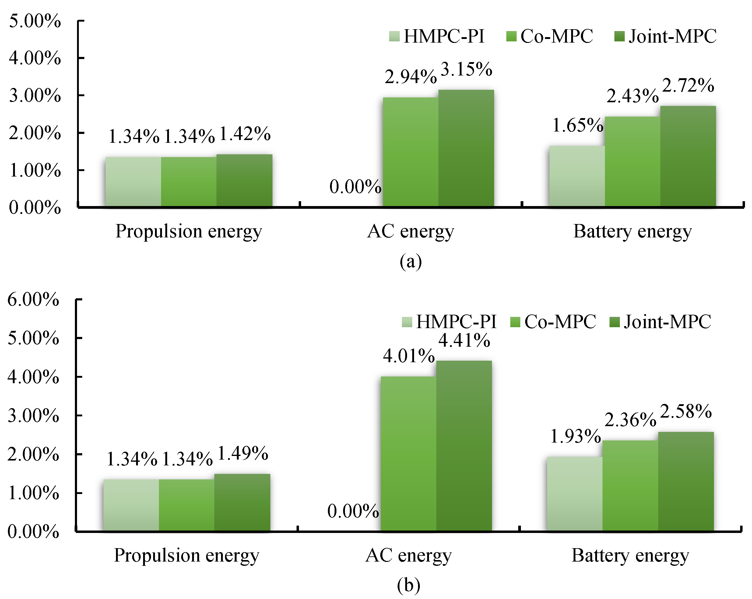
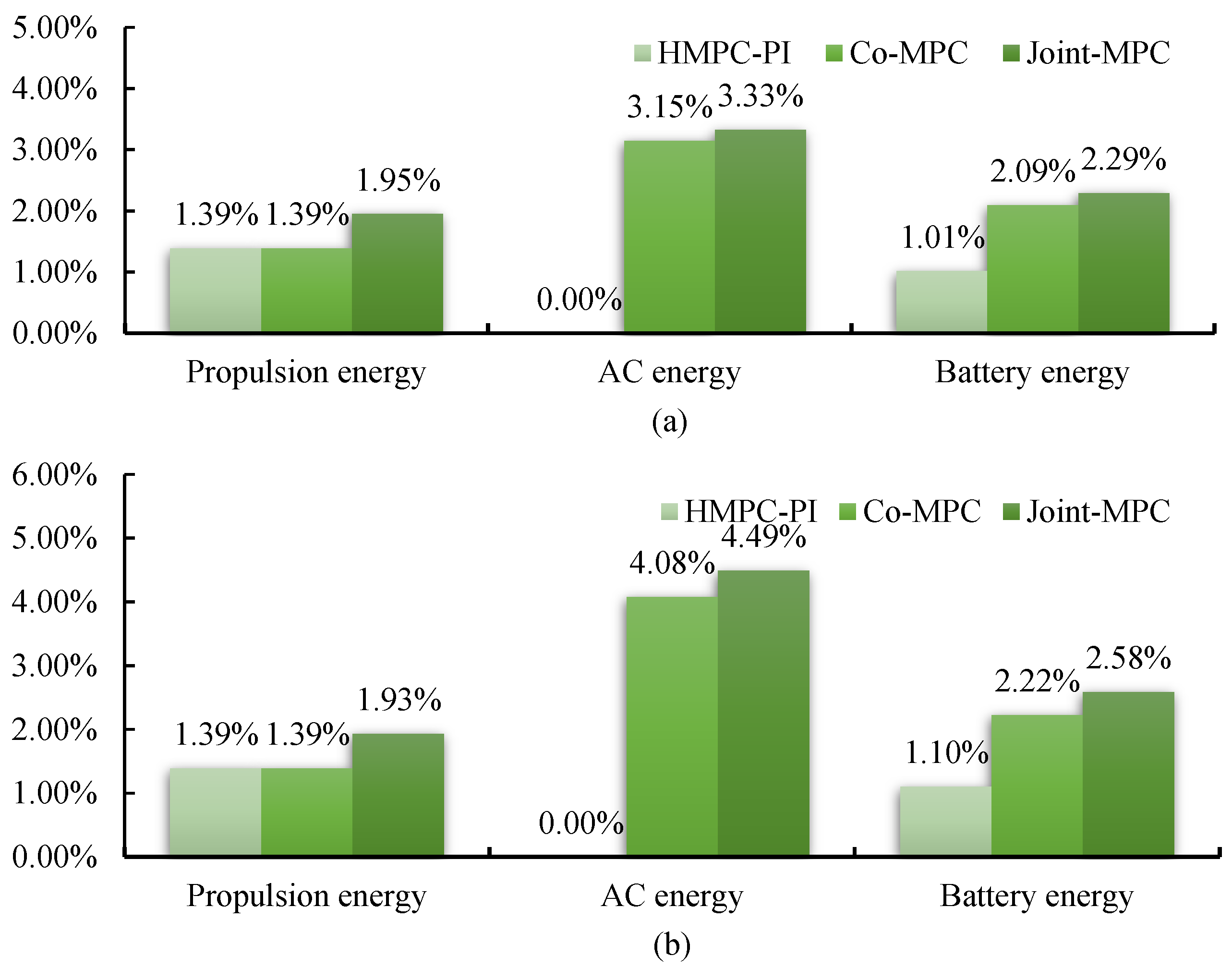
• Due to the integration of AC management, the proposed joint MPC ultimately reduces battery energy consumption by 0.65% to 1.48% compared to the HMPC-PI. Moreover, the thermal buffer is more effectively utilized in recirculation mode than in fresh-air mode.
• Both the joint MPC and co-MPC produce significant energy benefits while maintaining driving and thermal comfort. In particular, the total energy savings range from 2.09% to 2.72%, whereas the AC energy savings range from 2.94% to 4.49%.
• In comparison with the co-MPC, the joint MPC has higher energy benefits but also higher computational overhead. Hence, the co-MPC appears to be a suitable choice for real-time applications with limited computational power.

It is important to note that both the joint MPC and co-MPC are essentially nonlinear MPCs (NMPCs). To further reduce the computation time of NMPCs, solvers may be implemented that are better suited for real-time applications. Future work may focus on using a custom or a commercial solver that might be able to reduce the computation time of a classic NMPC, e.g., by applying real-time iterations [40]. Real-time solvers must also adhere to limited memory usage in order to be embedded in a hardware platform, which is also a subject for future study. Meanwhile, instead of passive air cooling, the battery pack requires active coolant cooling for heavier EVs [41]. Hence, in the future, battery thermal management will be incorporated into the design of an integrated propulsion and thermal management system for EVs.

References

1. Muratori, M.; Alexander, M.; Arent, D.; Bazilian, M.; Dede, E.M.; Farrell, J.; Gearhart, C.; Greene, D.; Jenn, A.; Keyser, M. The rise of electric vehicles—2020 status and future expectations. Prog. Energy 2021, 3, 022002. [Google Scholar] [CrossRef]
2. Santos, G.; Rembalski, S. Do electric vehicles need subsidies in the uk? Energy Policy 2021, 149, 111890. [Google Scholar] [CrossRef]
3. Wang, N.; Tang, L.; Pan, H. A global comparison and assessment of incentive policy on electric vehicle promotion. Sustain. Cities Soc. 2019, 44, 597–603. [Google Scholar] [CrossRef]
4. Pevec, D.; Babic, J.; Carvalho, A.; Ghiassi-Farrokhfal, Y.; Ketter, W.; Podobnik, V. A survey-based assessment of how existing and potential electric vehicle owners perceive range anxiety. J. Clean. Prod. 2020, 276, 122779. [Google Scholar] [CrossRef]
5. Vahidi, A.; Sciarretta, A. Energy saving potentials of connected and automated vehicles. Transp. Res. Part C Emerg. Technol. 2018, 95, 822–843. [Google Scholar] [CrossRef]
6. Dong, H.; Zhuang, W.; Chen, B.; Yin, G.; Wang, Y. Enhanced eco-approach control of connected electric vehicles at signal-ized intersection with queue discharge prediction. IEEE Trans. Veh. Technol. 2021, 70, 5457–5469. [Google Scholar] [CrossRef]
7. Gao, Y.; Yang, S.; Wang, X.; Li, W.; Hou, Q.; Cheng, Q. Cyber Hierarchy Multiscale Integrated Energy Management of Intel-ligent Hybrid Electric Vehicles. Automot. Innov. 2022, 5, 438–452. [Google Scholar] [CrossRef]
8. Ju, F.; Zhuang, W.; Wang, L.; Wang, Q. Iterative Dynamic Programming Based Model Predictive Control of Energy Efficient Cruising for Electric Vehicle with Terrain Preview; SAE Technical Paper; No.2020-01-0132; SAE: Warrendale, PA, USA, 2020. [Google Scholar]
9. Li, J.; Liu, Y.; Zhang, Y.; Lei, Z.; Chen, Z.; Li, G. Data-driven based eco-driving control for plug-in hybrid electric vehicles. J. Power Sources 2021, 498, 229916. [Google Scholar] [CrossRef]
10. Yang, J.; Xu, X.; Peng, Y.; Deng, P.; Wu, X.; Zhang, J. Hierarchical energy management of a hybrid propulsion system considering speed profile optimization. Energy 2022, 123098. [Google Scholar] [CrossRef]
11. Zulkefli, M.A.M.; Zheng, J.; Sun, Z.; Liu, H.X. Hybrid powertrain optimization with trajectory prediction based on inter-vehicle-communication and vehicle-infrastructure-integration. Transport. Res. C Emerg. Technol. 2014, 45, 41–63. [Google Scholar] [CrossRef]
12. Hu, J.; Shao, Y.; Sun, Z.; Wang, M.; Bared, J.; Huang, P. Integrated optimal eco-driving on rolling terrain for hybrid electric vehicle with vehicle-infrastructure communication. Transport. Res. C Emerg. Technol. 2016, 68, 228–244. [Google Scholar] [CrossRef]
13. Xu, S.; Li, S.E.; Cheng, B.; Li, K. Instantaneous feedback control for a fuel-prioritized vehicle cruising system on highways with a varying slope. IEEE Trans. Intell. Transp. Syst. 2016, 18, 1210–1220. [Google Scholar] [CrossRef]
14. Guo, L.; Zhang, X.; Zou, Y.; Han, L.; Du, G.; Guo, N.; Xiang, C. Co-optimization strategy of unmanned hybrid electric tracked vehicle combining eco-driving and simultaneous energy management. Energy 2022, 123309. [Google Scholar] [CrossRef]
15. Guo, Q.; Angah, O.; Liu, Z.; Ban, X.J. Hybrid deep reinforcement learning based eco-driving for low-level connected and automated vehicles along signalized corridors. Transp. Res. Part C Emerg. Technol. 2021, 124, 102980. [Google Scholar] [CrossRef]
16. Qi, C.; Zhu, Y.; Song, C.; Cao, J.; Xiao, F.; Zhang, X.; Xu, Z.; Song, S. Self-supervised reinforcement learning-based energy management for a hybrid electric vehicle. J. Power Sources 2021, 514, 230584. [Google Scholar] [CrossRef]
17. Cai, H.; Xu, X. Lateral Stability Control of a Tractor-Semitrailer at High Speed. Machines 2022, 10, 716. [Google Scholar] [CrossRef]
18. Xu, F.; Shen, T. Look-ahead prediction-based real-time optimal energy management for connected hevs. IEEE Trans. Veh. Technol. 2020, 69, 2537–2551. [Google Scholar] [CrossRef]
19. Ju, F.; Murgovski, N.; Zhuang, W.; Wang, Q.; Wang, L. Predictive Cruise Controller for Electric Vehicle to Save Energy and Extend Battery Lifetime. IEEE Trans. Veh. Technol. 2022; early access. [Google Scholar]
20. Uebel, S.; Murgovski, N.; Baker, B.; Sjöberg, J. A two-level mpc for energy management including velocity control of hybrid electric vehicles. IEEE Trans. Veh. Technol. 2019, 68, 5494–5505. [Google Scholar] [CrossRef]
21. Lajunen, A.; Yang, Y.; Emadi, A. Review of cabin thermal management for electrified passenger vehicles. IEEE Trans. Veh. Technol. 2020, 69, 6025–6040. [Google Scholar] [CrossRef]
22. Al-Wreikat, Y.; Serrano, C.; Sodre, J.R. Effects of ambient temperature and trip characteristics on the energy consumption of an electric vehicle. Energy 2022, 238, 122028. [Google Scholar] [CrossRef]
23. Vatanparvar, K.; Al Faruque, M.A. Path to eco-driving: Electric vehicle hvac and route joint optimization. IEEE Design Test. 2017, 35, 8–15. [Google Scholar] [CrossRef]
24. Wang, H.; Kolmanovsky, I.; Amini, M.R.; Sun, J. Model predictive climate control of connected and automated vehicles for improved energy efficiency. In Proceedings of the Annual American Control Conference, Milwaukee, WI, USA, 27–29 June 2018. [Google Scholar]
25. Wang, H.; Meng, Y.; Zhang, Q.; Amini, M.R.; Kolmanovsky, I.; Sun, J.; Jennings, M. Mpc-based precision cooling strategy (pcs) for efficient thermal management of automotive air conditioning system. In Proceedings of the IEEE Conference on Control Technology and Applications, Hong Kong, China, 19–21 August 2019. [Google Scholar]
26. Wang, H.; Amini, M.R.; Hu, Q.; Kolmanovsky, I.; Sun, J. Eco-cooling control strategy for automotive air-conditioning system: Design and experimental validation. IEEE Trans. Contr. Syst. Technol. 2020, 29, 2339–2350. [Google Scholar] [CrossRef]
27. Amini, M.R.; Wang, H.; Gong, X.; Liao-McPherson, D.; Kolmanovsky, I.; Sun, J. Cabin and battery thermal management of connected and automated hevs for improved energy efficiency using hierarchical model predictive control. IEEE Trans. Contr. Syst. Technol. 2019, 28, 1711–1726. [Google Scholar] [CrossRef]
28. Hu, Q.; Amini, M.R.; Kolmanovsky, I.; Sun, J.; Wiese, A.; Seeds, J.B. Multihorizon model predictive control: An application to integrated power and thermal management of connected hybrid electric vehicles. IEEE Trans. Contr. Syst. Technol. 2021, 30, 1052–1064. [Google Scholar] [CrossRef]
29. Liu, Y.; Zhang, J. Electric vehicle battery thermal and cabin climate management based on model predictive control. J. Mech. Des. 2021, 143, 031705. [Google Scholar] [CrossRef]
30. Zhao, S.; Mi, C.C. A two-stage real-time optimized ev battery cooling control based on hierarchical and iterative dynamic programming and mpc. IEEE Trans. Intell. Transport. Syst. 2021, 23, 11677–11687. [Google Scholar] [CrossRef]
31. Zhao, S.; Amini, M.R.; Sun, J.; Mi, C.C. A two-layer real-time optimization control strategy for integrated battery thermal management and hvac system in connected and automated hevs. IEEE Trans. Veh. Technol. 2021, 70, 6567–6576. [Google Scholar]
32. Chen, Y.; Kwak, K.H.; Kim, J.; Kim, Y.; Jung, D. Energy-efficient cabin climate control of electric vehicles using linear time-varying model predictive control. Optim. Control Appl. Meth. 2021, 1–25. [Google Scholar] [CrossRef]
33. Lohse-Busch, H.; Duoba, M.; Rask, E.; Meyer, M. Advanced Powertrain Research Facility Avta Nissan Leaf Testing and Analysis; Argonne National Laboratory: Lemont, IL, USA, 2012.
34. Burress, T. Benchmarking state-of-the-art technologies. In Proceedings of the 2013 US Department of Energy Hydrogen and Fuel Cells Program and Vehicle Technologies Program Annual Merit Review and Peer Evaluation Meeting, Arlington, VA, USA, 13–16 May 2013. [Google Scholar]
35. Kiss, T.; Chaney, L.; Meyer, J. New Automotive Air Conditioning System Simulation Tool Developed in Matlab/Simulink; Tech. Rep.; National Renewable Energy Lab.: Golden, CO, USA, 2013.
36. Kiss, T.; Lustbader, J. Comparison of the Accuracy and Speed of Transient Mobile a/c System Simulation Models; Tech. Rep.; National Renewable Energy Lab.: Golden, CO, USA, 2014.
37. Vatanparvar, K.; Al Faruque, M.A. Battery lifetime-aware automotive climate control for electric vehicles. In Proceedings of the ACM/EDAC/IEEE Design Automation Conference (DAC), San Francisco, CA, USA, 8–12 June 2015. [Google Scholar]
38. Andersson, J.A.; Gillis, J.; Horn, G.; Rawlings, J.B.; Diehl, M. Casadi: A software framework for nonlinear optimization and optimal control. Math. Program. Comput. 2019, 11, 1–36. [Google Scholar] [CrossRef]
39. Zhang, Q.; Li, S.E.; Deng, K. Automotive Air Conditioning: Optimization, Control and Diagnosis; Springer: Berlin/Heidelberg, Germany, 2016. [Google Scholar]
40. Diehl, M. Real-Time Optimization for Large Scale Nonlinear Processes. Ph.D. Thesis, University of Heidelberg, Heidelberg, Germany, 2001. [Google Scholar]
41. Ma, Y.; Ding, H.; Liu, Y.; Gao, J. Battery thermal management of intelligent-connected electric vehicles at low temperature based on nmpc. Energy 2021, 244, 122571. [Google Scholar] [CrossRef]
Figure 1. Schematic of the studied EV, including the propulsion system, AC system, and cabin thermal system. The AC system uses a refrigerant cycle with an electrically driven compressor for cooling. In the studied system, the battery pack is passively cooled by ambient air.
Actuators 11 00356 g001
Figure 2. Schematic of longitudinal dynamics.
Actuators 11 00356 g002
Figure 3. Power consumption and torque bounds of the motor. (a) Power consumption: measurements are represented by dots and the fitted polynomial by a surface; (b) Torque bounds of the motor, where the maximum and minimum torques of the motor are depicted by solid and dashed lines, respectively.
Actuators 11 00356 g003
Figure 4. Validation of the control-oriented AC model. Sinusoidal inputs to the AC system: (a) the target temperature of the wall of the evaporator and (b) the flow rate of the blower air. Outputs include (c) the temperature of the evaporator, (d) the air inlet temperature into the cabin, and (e) the air temperature in the cabin, as well as the power of two components: (f) the evaporator blower and (g) the compressor.
Actuators 11 00356 g004
Figure 5. Control structure of the co-MPC. Two different optimization goals are selected for the higher-layer and lower-layer MPCs.
Actuators 11 00356 g005
Figure 6. Speed results of the first case study. (a) Altitude profile of the expressway; (b) Speed trajectories for different methods; (c) Acceleration profiles of the co-MPC and joint MPC; (d) Jerk profiles of the co-MPC and joint MPC.
Actuators 11 00356 g006
Figure 7. Results of an LMPC update. (a) Input to the LMPC: P ^ prop ; (b) Cabin air temperature in two AC modes.
Actuators 11 00356 g007
Figure 8. Thermal results of the first case study, as well as a comparison of the different methods during a short period. (a) Cabin air temperature trajectory in fresh-air mode; (b) Cabin air temperature trajectory in recirculation mode. The comparison includes the (c) Blower rate; (d) Cabin air temperature; (e) Evaporator wall temperature target; (f) Increment of the blower rate; (g) AC power; (h) Propulsion power.
Actuators 11 00356 g008
Figure 9. Simulation results of the second case study in recirculation mode. (a) Altitude profile of the hilly road; (b) Speed trajectories for different methods; (c) Cabin air temperature trajectories for different methods.
Actuators 11 00356 g009
Figure 10. Energy benefits of the different methods compared to the CS-PI in the first case study. (a) Fresh-air mode; (b) Recirculation mode.
Actuators 11 00356 g010
Figure 11. Energy benefits of different methods compared to the CS-PI in the second case study. (a) Fresh-air mode; (b) Recirculation mode.
Actuators 11 00356 g011