Article

An Intelligent Process to Estimate the Nonlinear Behaviors of an Elasto-Plastic Steel Coil Damper Using Artificial Neural Networks

1
Department of Civil Engineering, Gwangju University, 277 Hyodeck-ro, Nam-gu, Gwangju 61743, Korea
2
R&D Center, Innose Tech Co., Ltd., 30, Songdomirae-ro, Yeonsu-gu, Incheon 21990, Korea
*
Author to whom correspondence should be addressed.
Actuators 2022, 11(1), 9; https://doi.org/10.3390/act11010009
Submission received: 2 November 2021 / Revised: 10 December 2021 / Accepted: 27 December 2021 / Published: 31 December 2021
(This article belongs to the Section Actuator Materials)

Abstract

:
This study developed a nonlinear behavior prediction model for elasto-plastic steel coil dampers (SCDs) using artificial neural networks (ANN). To train the ANN, first, the input and output data of the behavior of the elasto-plastic SCD was prepared. This study utilized the design parameters and load–displacement curves of the SCD to train the ANN. The elasto-plastic load–displacement curve of the SCD was obtained from simulation results using an ANSYS workbench. The design parameters (wire diameter, internal diameter, number of active windings, yield strength) of the SCD were defined as the input patterns, while the yield deformation, first stiffness, and second stiffness were output patterns. During learning of the neural network model, 60 datasets of the SCD were used as the learning pattern, and the remaining 21 were used to verify the model. Although this study used a small number of learning patterns, the ANN predicted accurate results for yield displacement, first stiffness, and second stiffness. In this study, the ANN was found to perform very well, predicting the nonlinear response of the SCD, compared with the values obtained from a finite element analysis program.

1. Introduction

External loads such as earthquakes and winds can induce large vibrations in long-span bridges and high-rise buildings, and these vibrations can last for a long time because of low damping. Isolation systems and dampers have accordingly been applied to these structures to improve their safety and usability by controlling the vibrations. The isolators and vibration control devices have been installed in both newly established structures and to seismic retrofit existing structures [1]. For example, flexible piping systems respond to seismic motion with large displacements. To reduce the large deformation produced by earthquakes, a damper can be installed in the piping system [2].
Seismic isolation devices are used to prevent vibration within a structure, and there are several types of dampers used to isolate structures, depending on the purpose. Such dampers can be classified into elasto-plastic dampers, viscous dampers, mass dampers, and friction dampers. Elasto-plastic dampers work by absorbing energy generated by the hysteretic deformation of a metal material, such as a steel bar, but the fatigue characteristics of repeated loading should be considered [3]. Viscous dampers are not highly affected by stiffness, so they can control from small to large vibrations. However, they are highly dependent on temperature [4,5]. Mass dampers such as a tuned mass damper were applied to various mechanical and civil structures [6,7,8]. A friction damper has the advantage that its damping force can be arbitrarily changed by the energy absorbed by friction [9].
Added damping and added stiffness (ADAS), triangular added damping and added stiffness (TADAS), unbonded bracing, loop-shaped damper, and lead damper devices were used in practice. ADAS is a device developed in the 1980s using concepts by Skinner [10], and TADAS is a device developed in Taiwan by modifying ADAS. However, these devices have problems such as fatigue destruction (ADAS, TADAS), device complexity, complex joined parts (unbonded bracing and loop-shaped damper), and difficult welding due to local stress concentration.
The elasto-plastic steel coil damper (SCD) overcomes the disadvantages of previous systems by distributing the internal stress of the damper during compression. Since the entire body of the SCD can be used for energy dissipation, the damping ratio is high, while the stress concentration is reduced, and the fatigue performance is also excellent. In addition, the SCD can be successfully applied to vibration control and isolated vibration devices [3].
If the wire diameter of SCD is small, it is possible to calculate the stress and the strain of the coil spring using equations for existing elastic mechanics theory with reasonable accuracy. If an SCD is subjected to a larger load, the wire diameter must be increased, and the cross-section of the wire changes from circular to various shapes. In such cases, it is not easy to analyze the behavior of the SCD, which exceeds the elastic limit.
Wahl [11] and SAE reports [12] described the materials, formulas, and theories for designing coil springs. Wahl [11] and Chandeler [13] reported a way to design coil springs based on stress correction factors. Saynor [14] analyzed several factors that affect the design, and John [15] introduced a method that allows the design to be performed directly without repeated calculations, by combining several formulae of coil springs. In addition, Anker [16,17,18] studied the characteristics of the coil spring according to changes in pitch and the outer diameter. Recently, Sato [19] verified the lateral deformation of a coil spring through numerical and experimental studies using a self-developed finite element analysis program. Suzuki [20] presented an analytical technique for coil springs using a general structure analysis program. Meanwhile, a study on the nonlinear characteristics of the coil spring was carried out by Bathe [21]. They constructed the nonlinear bending–deformation relationship of the coil spring using elasto-plastic and viscoelastic theory. In a study on the coil spring material, Sawanobori [22] analyzed the dynamic characteristics of coil springs according to the material properties of the steel, using a finite element method. Research using shape memory alloy was conducted by Kwon [23] and Lee [24], and Oh [25] investigated the design factors involved in using carbon-fiber-reinforced polymer (CFRP) for a light weight coil spring.
The SCD can reduce the vibration of the structure by producing the hysteretic damping by the nonlinear behavior with the material properties. Recently, the SCD has begun research to apply as a snubber to reduce vibration in the piping system of nuclear power plants [3]. To effectively reduce the vibration of the structure, the hysteretic behavior of the SCD should be accurately investigated. Therefore, this study proposes a methodology to precisely predict the nonlinear behavior of the SCD.
To design the SCD, it is necessary to develop a practical method to accurately predict nonlinear behavior. An artificial neural network (ANN) can be used to develop a design model for an elasto-plastic SCD. The ANN is very effective when considering various inputs and outputs without mathematical calculations compared to existing regression analysis. It is generally used to estimate an unknown function while relying on many inputs. The first neural network model was proposed in 1943 by McCulloch and Pitts [26]. Since then, ANN have become a new alternative approach for pattern recognition in many fields of application, including biology [27], economics [28], environment [29], manufacturing [30], medicine [31], and the military [32]. In civil engineering, neural networks have been applied to assess the damage to a structure, analyze the behavior of the material, design the optimization of the structure, monitor the groundwater level, control the structural vibration, assess the structural reliability, and predict concrete compressive strength [23,24,25,26,27,28,29,30,31,32,33,34,35,36,37,38,39,40,41,42].
This study used an ANN to predict the hysteretic behavior of the elasto-plastic SCDs. To train the ANN, the input and output nonlinear behavior data of the SCD had to be prepared. For this purpose, design parameters and load–displacement curves were used for the ANN learning process. The load–displacement curves of the SCD were obtained from a simulation using ANSYS Workbench software.
This paper introduces the structure of the ANN used in this study. The design parameters of the SCD and the acquisition of the load–displacement curve were obtained using a large number of numerical analyses. The paper discusses the process and results for predicting the nonlinear behavior of an elasto-plastic SCD using the ANNs.

2. Analytical Model of the Elasto-Plastic SCD

2.1. Mechanical Behavior of Coil Spring

When a coil spring is loaded by compressive force, it develops the internal forces shown in Figure 1. As is well known, the spring stiffness in the elastic range, k e is represented by Equation (1).
k e = G × d 4 8 × N e × D 3
where G is the shear modulus, d is the wire diameter, N e is the number of effective windings, and D is the diameter of the spring [3].
The SCD is deformed in a nonlinear way beyond the elastic range with k 2 of stiffness, as shown in Figure 2. The elastic stiffness can be calculated using Equation (1), but the post-yield stiffness cannot be easily derived by theoretical formulation.

2.2. Finite Element Model

This study performed numerical analyses to determine the design parameters of the SCD. Finite element analysis software, ANSYS, was used for the numerical analyses, so the nonlinear behaviors of the elasto-plastic SCD could be confirmed. Table 1 shows the design parameters used for the nonlinear analyses of the SCD.
The SCD models used in the analysis are shown in Figure 3, Figure 4 and Figure 5. The wire diameters of the SCDs used in the analysis were 6 mm, 8 mm, and 10 mm. The spring diameters were 40 mm, 50 mm, 60 mm, and the yield strengths of the steel material were 400 MPa, 580 MPa, and 650 MPa. The number of effective windings of coils was four, five, and six, respectively. Therefore, the total number of cases used in the analysis was 81 (3 × 3 × 3 × 3 = 81).

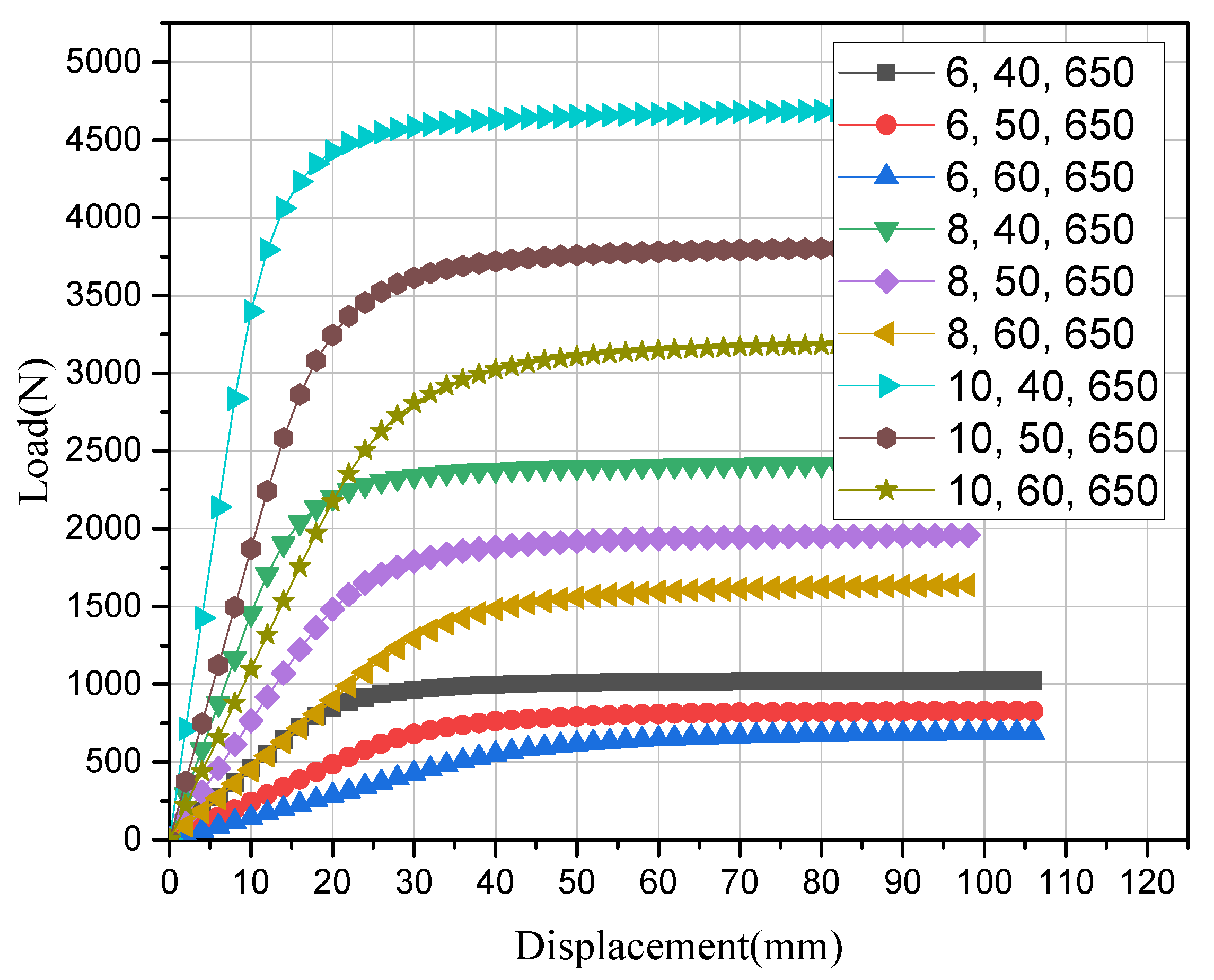
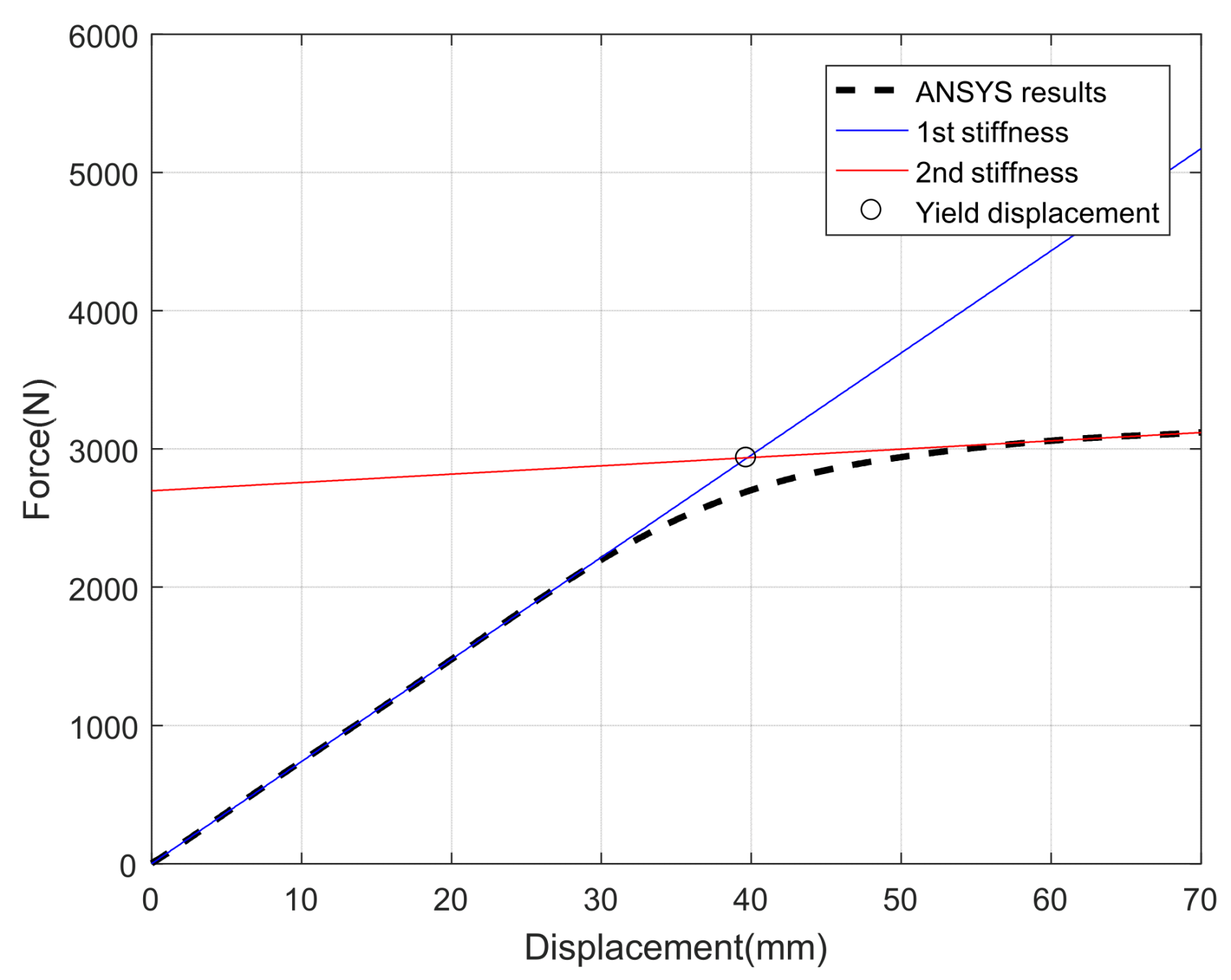
2.3. Loading Test Simulation

ANSYS Workbench was used to simulate the nonlinear behavior of the SCD. The analysis case shown in Table 1 was performed to simulate a loading test to confirm the nonlinear behavior. The enforced displacement was input to deform the spring, and the displacement was set from 0 to 70 mm according to each model. The three-dimensional solid element (SOLID186) was used to construct the analytical model, and the bi-linear material model was applied to simulate the nonlinear behavior of the material (see Figure 6).
All of the SCD had a minimum free length of 130 mm. Figure 7, Figure 8 and Figure 9 show the load–displacement curves for yield strengths of 400 MPa, 580 MPa, and 650 MPa when the number of effective coils was 5. In Figure 7, Figure 8 and Figure 9, the wire diameters were between 6 and 10 mm, and the spring diameters varied from 40 to 60 mm. A total of 81 datasets, including the load–displacement data in Figure 7, Figure 8 and Figure 9, were used to predict the nonlinear behavior of the SCD using the ANNs.

3. Estimation of the Elasto-Plastic Behavior of SCDs Using ANN

3.1. Objective of Estimation

While designing the coil spring, the wire diameter, spring diameter, number of effective windings, and yield strength were determined as the design parameters. This study utilized the design parameters of the SCD and the loading test simulation results as learning patterns (learning data sets) for the ANNs. The nonlinear load–displacement curve of the elasto-plastic SCD was predicted using the learned ANNs. The design parameters of the SCD were defined as input patterns, while the yield displacement ( δ y ), first stiffness ( k 1 s t ), and second stiffness ( k 2 n d ) of the SCD were assumed to be output patterns. Therefore, a total of three neural network models were used to predict the yield displacement, first stiffness, and second stiffness. The elasto-plastic behavior of the SCD can be calculated using the predicted results.

3.2. Estimation Procedure

The flow chart for the predicted load–displacement curve of the SCD is shown in Figure 10. Prior to constructing the ANN model, the first stiffness, the second stiffness, and the yield displacement were calculated according to each SCD using the ANSYS analysis results. Here, yield displacement was defined as the displacement where the first stiffness and the second stiffness cross. An ANN1 model was constructed by inputting the wire diameter, central diameter, number of effective windings, and yield strength and by outputting the yield displacement. ANN2 and ANN3 models were constructed by models outputting the first stiffness and second stiffness, respectively, under the same input set. Finally, the elasto-plastic responses of the SCDs were calculated using the predicted yield displacement, first stiffness, and second stiffness.
Figure 11 shows an example where the yield displacement was selected using the first stiffness and second stiffness. Here, the black dashed line is the load–displacement curve of the SCD obtained by ANSYS analysis. The blue line and red line show the first stiffness and second stiffness, respectively. The black circle at the point where the two lines intersect indicates the yield displacement.

3.3. Artificial Neural Network

It is known that ANNs can effectively handle input–output relationships that are difficult to construct using mathematically strict models. In order to build the ANN, this study constitutes an input layer, hidden layer, and output layer, as shown in Figure 12. The input layer is a distribution layer for inputting data to predict the elasto-plastic behavior of the SCD, and the hidden layer is the weighted matrix connecting the input layer to the output layer. The output layer outputs the prediction result through the operation in the input layer and the hidden layer. The weighting matrix of the hidden layer is updated using the error between the predicted result and the target value. This repetitive procedure is the ANN learning process. The learning process of the neural network is further described in the following paragraphs.
Since the learning process of the artificial neural networks is described in detail in several papers, this paper briefly explained [38]. Assuming that the input of the input layer is I h , the output of the hidden layer can be represented by the following equation.
o i 1 = f 1 ( n e t i 1 )           ( i = 1 ,   2 ,   ,   n 2 )
where f 1 and n e t i 1 are the activation function and the net input of the j th node of the hidden layer, respectively. The net input is
n e t i 1 = h = 1 n 1 W i h 1 I h + b i 1
where W i h 1 is the connection weight matrix between the input and hidden layers and b i 1 is the bias of the hidden layer. The relationship between the net input of the hidden layer and the output of the output layer is as follows:
o j 2 = f 2 ( n e t j 2 )         j = 1 ,   2 ,   ,   n 3  
where f 2 and n e t j 2 are the active function and the net input of the j th node of the output layer. The net input is as follows:
n e t j 2 = i = 1 n 2 W j i 2 o i 1 + b j 2
where W j i 2 is the connection weight matrix between the hidden and output layers and b j 2 is the bias of the output layer.
The weights and biases should be modified so that the learning algorithm of the ANN predicts the desired output. This process, the so-called learning or training, is accomplished by minimizing the error function, which is defined as follows:
e r r o r = | o d o j 2 | 2
where o d and o j 2 are the desired output and the predicted output.

4. Verification of the ANN Model

The design parameters of the SCD were estimated using the proposed ANN. The estimation performance was verified by comparing the estimation results to the finite element analysis results for the loading test simulation. The nonlinear behavior of the SCD was calculated using the predicted results. To train the neural network models, among the 81 datasets for the SCD, 60 were used for the learning pattern, and the remaining 21 were used for verification of the model.

4.1. Learning Process of ANN Models

Table 2, Table 3 and Table 4 show the sample data for 10 learning patterns among 60 patterns for ANN1, ANN2, and ANN3, respectively. In Table 2, the wire diameter, spring diameter, yield strength, and number of effective windings were used as the input pattern of ANN1, and the yield displacement was defined as an output pattern of ANN1. In Table 2 and Table 3, the first stiffness and second stiffness were defined as the output patterns of ANN2 and ANN3, respectively. In order to assign the same weighting, the design parameters were normalized from 0.1 to 0.9. The TANSIG function and PURELIN function were used as the activate functions in the hidden and output layer, respectively [43]. In addition, 0.95 was selected as the initial learning rate, the error rate defined by the mean square error (MSE) was 1.0 × 10⁻⁶, and the number of learnings was set to 400 times.
Figure 13 shows the convergence process of MSE during the learning process for estimation of the yield displacement. Although it did not converge to the target error 1.0 × 10⁻⁶, it can be seen that MSE is stably converged at epoch 100 or higher.

4.2. Estimation Results Obtained with the ANN Models

In order to validate the ANN models for estimating the nonlinear response of the elasto-plastic SCD, 21 patterns were randomly extracted from the 81 analysis results. The extracted data (21 data sets) were used to test the performance of the ANN models.
Figure 14, Figure 15 and Figure 16 show the results of predicted yield displacement, first stiffness, and second stiffness of the SCD using ANNs. The blue bar graph in Figure 14a shows the target yield displacement for 21 patterns, and the yellow bar graph represents the yield displacement predicted by the ANN1. Figure 14b exhibits a bar graph showing the prediction error for 21 patterns, which had a maximum error rate of 7%. Figure 15 and Figure 16 show the result and error for the first stiffness and second stiffness predictions, respectively.
The predicted results for yield displacement, first stiffness, and second stiffness using the ANN are summarized in Table 5, Table 6 and Table 7. Table 5 shows the test patterns, target yield displacements, and estimated yield displacements from the ANNs. The errors for the target yield displacements and the predicted yield displacements were about −0.4% to −7.5%. Table 6 shows the prediction results for first stiffness. The errors of the target stiffness and the predicted stiffness were 0% to 8.1%. Table 7 shows the prediction results for the second stiffness and the errors 1.5% to −19.7%. The graphs indicate that the errors in Table 7 seem to be relatively larger than those in Table 6. The reason is that the value of the second stiffness is relatively small. For example, in the eighth result in Table 7, the error is −19.7%; however, the target stiffness and the predicted stiffness are 0.87 n/mm and 1.04 n/mm, respectively.

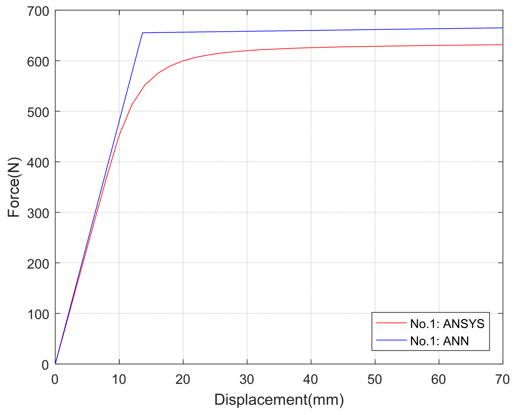
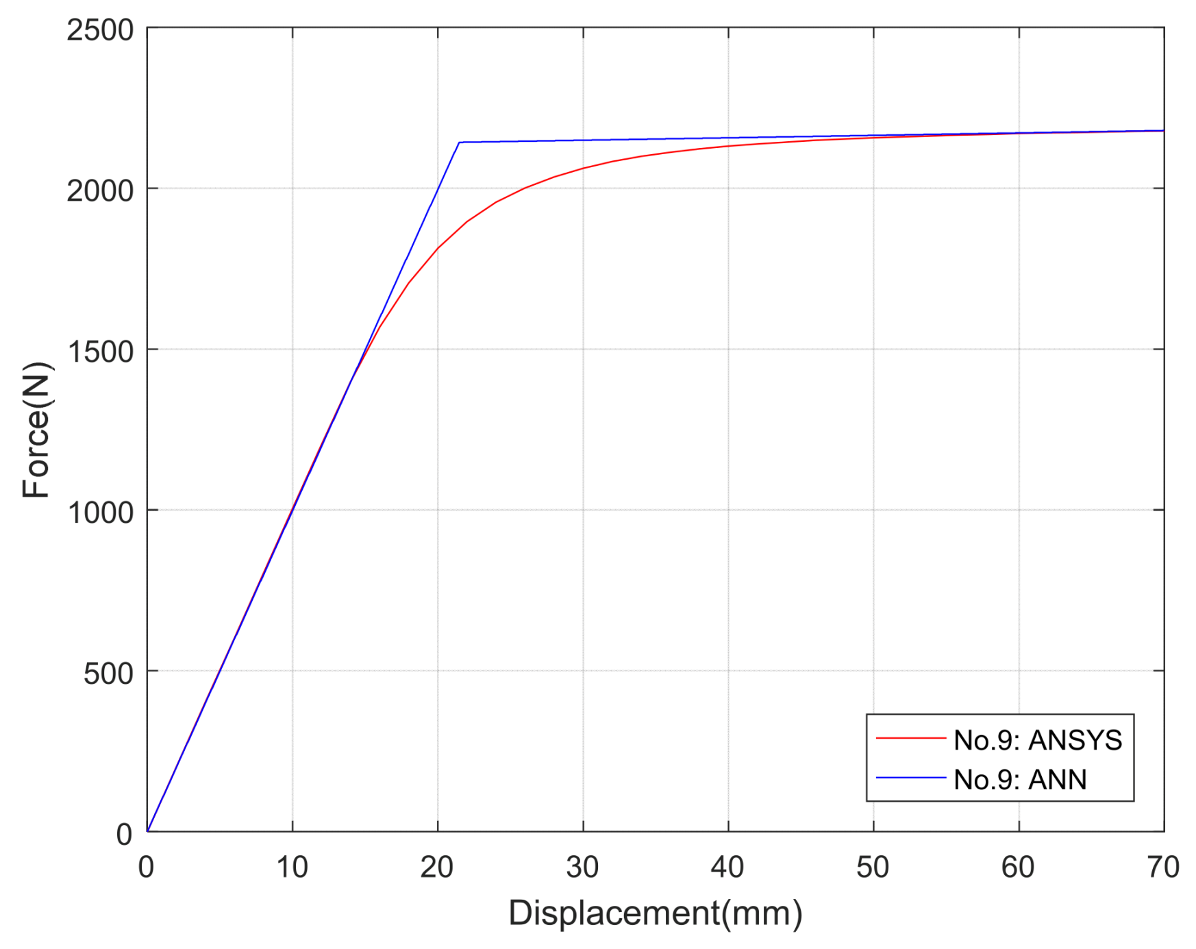
4.3. Comparison of Nonlinear Response Results

Figure 17, Figure 18, Figure 19 and Figure 20 show the load–displacement curves of the SCD obtained from ANSYS and ANNs. The red line in the figures indicates the load test simulation result from the ANSYS program. The blue line represents the estimated nonlinear response from the ANN models. The predicted nonlinear response was calculated by combining the yield displacement, the first stiffness, and the second stiffness estimated by ANNs. Figure 17 shows the load–displacement curves for the parameters (4 mm, 40 mm, 400 MPa, and 4) of the first data in Table 5, Table 6 and Table 7. The errors for the predicted yield displacement, first stiffness, and second stiffness were −1.0%, −4.3%, and −18.3%, respectively. Clearly, the errors for the first and second stiffness were large relatively. Figure 18 shows the load–displacement curves for parameters (6 mm, 50 mm, 650 MPa, and 5) of the fifth data in Table 5, Table 6 and Table 7. The errors for the predicted yield displacement and first and second stiffnesses were 0.8%, 8.1%, and −1.2%, respectively. The error for the first stiffness was larger than the target value. The yield displacement and the second stiffness were exactly predicted; however, the estimated load–displacement curve did not match the target curve due to the influence of the first stiffness. Figure 19 shows the results for the seventh data in Table 5, Table 6 and Table 7. The errors for each predicted result were −0.4%, −0.7%, and −5.7%, respectively. The error for the second stiffness was relatively large; however, it shows a trend highly similar to the ANSYS results. Finally, Figure 20 shows the results of the elasto-plastic coil damper for the ninth data in Table 5, Table 6 and Table 7. The errors of −0.8%, 0.6%, and 3.8% show they were accurately predicted, and the load–displacement curves are also similar to the ANSYS results.
From Table 5, Table 6 and Table 7, Figure 17, Figure 18, Figure 19 and Figure 20, the overall behavior estimated by ANN tends to be very close to the nonlinear behavior obtained using ANSYS, when the first stiffness estimated by the ANN is accurately predicted. It is also noted that the entire nonlinear stiffness of SCD could be matched with the numerical analysis results when the yield point is accurately estimated. Since the second stiffness is relatively small compared to the first stiffness, it does not largely affect in the estimated response.

5. Conclusions

This study developed a nonlinear behavior prediction model for the design of elasto-plastic SCDs, using ANNs. In order to construct patterns for the ANNs learning process, the ANSYS program was used to model the elasto-plastic SCD. Then, a set of numerical simulation was performed to confirm the nonlinear behavior of the SCDs. The design parameters of the SCD, including wire diameter, internal diameter, the number of effective windings, and yield strength were defined as the input patterns, while the yield displacement ( δ y ), first stiffness ( k 1 s t ), and second stiffness ( k 2 n d ) of the elasto-plastic coil damper were assumed to be the output patterns of the ANNs. For ANN model learning, from the total 81 datasets, 60 elasto-plastic coil damper data were used as the learning patterns, and the remaining 21 data were used for model verification.
Although relatively few learning patterns were used in this study, the results of the ANNs showed precise prediction results for yield displacement, first stiffness, and second stiffness. In addition, the performance of the ANN’s predicted nonlinear response was also found to be sufficient compared to the ANSYS analysis results. These results confirmed that the nonlinear behavior prediction model using ANNs proposed in this study could predict the behavior of the elasto-plastic SCD coil damper.
In further study, the number of loading test data for the elasto-plastic dampers will be increased to improve the accuracy of the ANN model.

Author Contributions

Conceptualization, S.G.C. and S.C.; methodology, S.C.; software, S.G.C.; validation, S.G.C. and S.C.; formal analysis, S.C.; investigation, S.G.C.; resources, S.G.C.; writing—original draft preparation, S.C.; writing—review and editing, S.G.C. and S.C.; project administration, S.G.C.; funding acquisition, S.G.C. and S.C. All authors have read and agreed to the published version of the manuscript.

Funding

This research was funded by Gwangju University in 2021 and the Ministry of Trade, Industry & Energy (No. 20181520102780), Korea.

Institutional Review Board Statement

Not applicable.

Informed Consent Statement

Not applicable.

Data Availability Statement

The data presented in this study are available on request from the corresponding author.

Acknowledgments

This study was conducted with the assistance of research funds from Gwangju University in 2021 and the Korea Institute of Energy Technology Evaluation and Planning (KETEP) (No. 20181520102780).

Conflicts of Interest

The authors declare no conflict of interest.

References

  1. JAVIT. Overview of Vibration Technologies 2010; Japan Association for Vibration Technologies: Takanawa, Japan, 2011. [Google Scholar]
  2. Chang, S.; Sun, W.; Cho, S.G.; Kim, D. Vibration Control of Nuclear Power Plant Piping System Using Stockbridge Damper under Earthquakes. Sci. Technol. Nucl. Install. 2016, 2016, 5014093. [Google Scholar] [CrossRef] [Green Version]
  3. Cho, S.G.; Furuya, O.; Kurabayashi, H. Enhancement of seismic resilience of piping systems in nuclear power plants using steel coil damper. Nucl. Eng. Des. 2019, 350, 147–157. [Google Scholar] [CrossRef]
  4. Ge, T.; Huang, X.-H.; Guo, Y.-Q.; He, Z.-F.; Hu, Z.-W. Investigation of Mechanical and Damping Performances of Cylindrical Viscoelastic Dampers in Wide Frequency Range. Actuators 2021, 10, 71. [Google Scholar] [CrossRef]
  5. Hansu, O.; Güneyisi, E. Comparison of Novel Seismic Protection Devices to Attenuate the Earthquake Induced Energy. Actuators 2021, 10, 73. [Google Scholar] [CrossRef]
  6. Chang, S. Active Mass Damper for Reducing Wind and Earthquake Vibrations of a Long-Period Bridge. Actuators 2020, 9, 66. [Google Scholar] [CrossRef]
  7. Elias, S.; Matsagar, V. Seismic vulnerability of a non-linear building with distributed multiple tuned vibration absorbers. Struct. Infrastruct. Eng. 2019, 15, 1103–1118. [Google Scholar] [CrossRef]
  8. Elias, S.; Rupakhety, R.; De Domenico, D.; Olafsson, S. Seismic response control of bridges with nonlinear tuned vibration absorbers. Structures 2021, 34, 262–274. [Google Scholar] [CrossRef]
  9. Le, L.M.; Van Nguyen, D.; Chang, S.; Kim, D.; Cho, S.G.; Nguyen, D.-D. Vibration control of jacket offshore wind turbine subjected to earthquake excitations by using friction damper. J. Struct. Integr. Maint. 2019, 4, 1–5. [Google Scholar] [CrossRef]
  10. Skinner, R.I.; Kelly, J.M.; Heine, A.J. Hysteresis dampers for earthquake resistant structures. Earthq. Eng. Struct. Dyn. 1974, 3, 287–296. [Google Scholar] [CrossRef]
  11. Wahl, A.M. Mechanical Springs; McGraw-Hill Book, Co.: New York, NY, USA, 1966. [Google Scholar]
  12. SAE Inc. Manual on Design and Application of Helical and Spiral Springs; HSJ795; SAE International: Warrendale, PA, USA, 1992. [Google Scholar]
  13. Chandeler, R.V. Direct procedure for helical spring design. Mach. Des. 1961, 131. [Google Scholar]
  14. Sayhor, D. Helical coil spring design. Engineering 1986, 131. [Google Scholar]
  15. John, R.C. Short cut for designing helical springs. Mach. Des. 1979, 22, 92–93. [Google Scholar]
  16. Ancker, C.J.; Goodier, J.N. Pitch and curvature corrections for helical springs. J. Appl. Mech. 1958, 25, 466–470. [Google Scholar] [CrossRef]
  17. Ancker, C.J.; Goodier, J.N. Theory of pitch and curvature corrections for the helical spring-Ⅰ (tension). J. Appl. Mech. 1958, 25, 471–483. [Google Scholar] [CrossRef]
  18. Ancker, C.J.; Goodier, J.N. Theory of pitch and curvature corrections for the helical spring-Ⅱ (torsion). J. Appl. Mech. 1958, 25, 484–495. [Google Scholar] [CrossRef]
  19. Sato, S.; Taguchi, K.; Adachi, R.; Nakatani, M. Strength characteristics of ceramic springs. Trans. Jpn. Soc. Spring Eng. 1997, 55–60. [Google Scholar] [CrossRef] [Green Version]
  20. Suzuki, S.; Kamiya, S.; Imaizumi, T.; Sanada, Y. Approaches to minimizing side force of helical coil springs in suspension design. Trans. Jpn. Soc. Spring Eng. 1996, 1996, 19–26. [Google Scholar] [CrossRef]
  21. Bathe, K.J.; Ozdemir, H. Elasto-plastic large deformation static and dynamic analysis. Comput. Struct. 1976, 6, 81–92. [Google Scholar]
  22. Sawanobori, T.; Nakamura, M. The analysis of static stress in coil springs with nonlinearity. Trans. Jpn. Soc. Mech. Eng. Ser. C 1985, 51, 3105–3108. [Google Scholar] [CrossRef] [Green Version]
  23. Kwon, H.K.; Choi, C.S.; Chung, I.S. Helical coil springs property in Cu-Zn-Al shape memory alloy. J. Korean Soc. Heat Treat. 1996, 9, 187–197. [Google Scholar]
  24. Lee, J.-G.; Ahn, S.-M.; Cho, K.-J.; Cho, M. The Prediction of Nonlinear behavior of Double Coil Shape Memory Alloy Spring. J. Comput. Struct. Eng. Inst. Korea 2012, 25, 347–354. [Google Scholar] [CrossRef] [Green Version]
  25. Oh, S.H.; Choi, B.L. Analytical and Experimental Study for Development of Composite Coil Springs. Trans. Korean Soc. Mech. Eng. A 2014, 38, 31–36. [Google Scholar] [CrossRef] [Green Version]
  26. Mcculloch, W.S.; Pitts, W. A logical calculus of the ideas immanent in nervous activity. Bull. Math. Biophys. 1943, 5, 115–133. [Google Scholar] [CrossRef]
  27. Darsey, J.A.; Griffin, W.O.; Joginipelli, S.; Melapu, V.K. Architecture and Biological Applications of Artificial Neural Networks: A Tuberculosis Perspective. Methods Mol. Biol. 2015, 1260, 269–283. [Google Scholar] [CrossRef] [PubMed]
  28. Calvo-Pardo, H.F.; Mancini, T.; Olmo, J. Neural Network Models for Empirical Finance. J. Risk Financial Manag. 2020, 13, 265. [Google Scholar] [CrossRef]
  29. Lin, Y.-K.; Su, M.-C.; Hsieh, Y.-Z. The Application and Improvement of Deep Neural Networks in Environmental Sound Recognition. Appl. Sci. 2020, 10, 5965. [Google Scholar] [CrossRef]
  30. Wang, P.-H.; Lin, G.-H.; Wang, Y.-C. Application of Neural Networks to Explore Manufacturing Sales Prediction. Appl. Sci. 2019, 9, 5107. [Google Scholar] [CrossRef] [Green Version]
  31. Drywień, M.; Górnicki, K.; Górnicka, M. Application of Artificial Neural Network to Somatotype Determination. Appl. Sci. 2021, 11, 1365. [Google Scholar] [CrossRef]
  32. Bistron, M.; Piotrowski, Z. Artificial Intelligence Applications in Military Systems and Their Influence on Sense of Security of Citizens. Electronics 2021, 10, 871. [Google Scholar] [CrossRef]
  33. Feng, M.Q.; Bahng, E.Y. Damage assessment of jacketed RC columns using vibration tests. J. Struct. Eng. 1999, 125, 265–271. [Google Scholar] [CrossRef]
  34. Ghaboussi, J.; Joghataie, A. Active Control of Structures Using Neural Networks. J. Eng. Mech. 1995, 121, 555–567. [Google Scholar] [CrossRef]
  35. Adeli, H.; Park, H.S. A neural dynamics model for structural optimization—Theory. Comput. Struct. 1995, 57, 383–390. [Google Scholar] [CrossRef]
  36. Ranjithan, S.; Eheart, J.W.; Garrett, J.H. Neural network-based screening for groundwater reclamation under uncertainty. Water Resour. Res. 1993, 29, 563–574. [Google Scholar] [CrossRef]
  37. Chen, H.M.; Tsai, K.H.; Qi, G.Z.; Yang, J.C.S.; Amini, F. Neural Network for Structure Control. J. Comput. Civ. Eng. 1995, 9, 168–176. [Google Scholar] [CrossRef]
  38. Chang, S.; Sung, D. Modal-Energy-Based Neuro-Controller for Seismic Response Reduction of a Nonlinear Building Structure. Appl. Sci. 2019, 9, 4443. [Google Scholar] [CrossRef] [Green Version]
  39. Mase, H.; Sakamoto, M.; Sakai, T. Neural Network for Stability Analysis of Rubble-Mound Breakwaters. J. Waterw. Port, Coastal, Ocean Eng. 1995, 121, 294–299. [Google Scholar] [CrossRef]
  40. Kim, D.H.; Park, W.S. Neural network for design and reliability analysis of rubble mound breakwaters. Ocean Eng. 2005, 32, 1332–1349. [Google Scholar] [CrossRef]
  41. Kim, J.-I.; Kim, D.K.; Feng, M.Q.; Yazdani, F. Application of Neural Networks for Estimation of Concrete Strength. J. Mater. Civ. Eng. 2004, 16, 257–264. [Google Scholar] [CrossRef]
  42. Kim, D.K.; Lee, J.J.; Lee, J.H.; Chang, S.K. Application of prediction of probabilistic neural networks of concrete strength. J. Mater. Civ. Eng. 2005, 17, 353–362. [Google Scholar] [CrossRef]
  43. Dorofki, M.; Elshafie, A.H.; Jaafar, O.; Karim, O.A.; Mastura, S. Comparison of artificial neural network transfer functions abilities to simulate extreme runoff data. Int. Proc. Chem. Biol. Environ. Eng. 2012, 2012, 39–44. [Google Scholar]
Figure 1. Forces in a compressive spring [3].
Actuators 11 00009 g001
Figure 2. Force–displacement relationship.
Actuators 11 00009 g002
Figure 3. SCDs according to wire diameters: (a) 6 mm; (b) 8 mm; (c) 10 mm.
Actuators 11 00009 g003
Figure 4. SCDs according to internal diameters: (a) 40 mm; (b) 50 mm; (c) 60 mm.
Actuators 11 00009 g004
Figure 5. SCDs according to the number of active coils: (a) 4; (b) 5; (c) 6.
Actuators 11 00009 g005
Figure 6. Stress–strain curve (580 MPa).
Actuators 11 00009 g006
Figure 7. Load–displacement curves of SCDs (n = 5).
Actuators 11 00009 g007
Figure 8. Load–displacement curves of SCDs (n = 5).
Actuators 11 00009 g008
Figure 9. Load–displacement curves of SCDs (n = 5).
Actuators 11 00009 g009
Figure 10. Flow chart for estimating the elasto-plastic response of the SCD.
Actuators 11 00009 g010
Figure 11. Yield point on the nonlinear response of SCD.
Actuators 11 00009 g011
Figure 12. Structure of ANN [38].
Actuators 11 00009 g012
Figure 13. Convergence process of MSE.
Actuators 11 00009 g013
Figure 14. Estimated yield displacement results: (a) comparison of yield displacement; (b) error.
Actuators 11 00009 g014aActuators 11 00009 g014b
Figure 15. Estimated first stiffness results: (a) comparison of first stiffness; (b) error.
Actuators 11 00009 g015
Figure 16. Estimated second stiffness results: (a) comparison of second stiffness; (b) error.
Actuators 11 00009 g016aActuators 11 00009 g016b
Figure 17. Estimated load–displacement curve (first coil damper).
Actuators 11 00009 g017
Figure 18. Estimated load–displacement curve (fifth coil damper).
Actuators 11 00009 g018
Figure 19. Estimated load–displacement curve (seventh coil damper).
Actuators 11 00009 g019
Figure 20. Estimated load–displacement curve (ninth coil damper).
Actuators 11 00009 g020
Table 1. Design parameters of SCD.
ParametersSymbolsValues
Wire diameterd (mm)6810
Spring diameterD (mm)405060
Yield strengthfy (MPa)400580650
Number of effective windingsn (number)456
Table 2. Input and output patterns of ANN1.
Wire Diameter
(mm)
Internal
Diameter (mm)
Yield Strength
(MPa)
Number of Active CoilsYield Displacement (mm)
640580419.5
840400410.1
860650434.4
1060580425.3
660400535.4
850650530.4
1050580522.0
650400630.2
840650623.7
1040580617.0
Table 3. Input and output patterns of ANN2.
Wire Diameter
(mm)
Internal
Diameter (mm)
Yield Strength
(MPa)
Number of Active CoilsFirst Stiffness
(n/mm)
640580446.1
8404004145.8
860650444.9
10605804109.7
660400511.5
850650561.9
10505805151.5
650400616.4
8406506100.4
10405806246.0
Table 4. Input and output patterns of ANN3.
Wire Diameter
(mm)
Internal
Diameter (mm)
Yield Strength
(MPa)
Number of Active CoilsSecond Stiffness
(n/mm)
64058040.28
84040040.36
86065041.93
106058041.47
66040050.51
85065051.59
105058051.35
65040060.38
84065061.11
104058061.10
Table 5. Estimated results of ANN1.
Wire
Diameter
(mm)
Internal
Diameter
(mm)
Yield Strength
(MPa)
Number of Active CoilsYield Displacement (mm)
TargetEstimationError (%)
640400413.5013.64−1.0
660650443.6044.68−2.5
860580431.2031.020.6
1060400417.7019.03−7.5
650650539.2038.890.8
850580527.4026.254.2
1050400515.4015.46−0.4
640650631.3032.89−5.1
840580621.3021.46−0.8
1040400611.8011.641.3
Table 6. Estimated results of ANN2.
Wire
Diameter
(mm)
Internal
Diameter
(mm)
Yield Strength
(MPa)
Number of Active Coils1st Stiffness (n/mm)
TargetEstimationError (%)
640400446.0648.06−4.3
660650414.2413.455.5
860580444.9045.58−1.5
10604004109.66109.420.2
650650519.6018.008.1
850580561.9461.870.1
10504005151.47152.58−0.7
640650631.7131.710.0
8405806100.4399.810.6
10404006246.00245.640.1
Table 7. Estimated results of ANN3.
Wire
Diameter
(mm)
Internal
Diameter
(mm)
Yield Strength
(MPa)
Number of Active Coils2nd Stiffness (n/mm)
TargetEstimationError (%)
64040040.150.17−18.3
66065041.751.93−10.0
86058041.271.251.7
106040040.530.56−5.4
65065051.401.42−1.2
85058051.070.9411.8
105040050.550.58−5.7
64065060.871.04−19.7
84058060.790.763.8
104040060.660.651.5
Publisher’s Note: MDPI stays neutral with regard to jurisdictional claims in published maps and institutional affiliations.

