1. Introduction
With the development of robotics, robotic applications are becoming more and more widespread. However, in many applications, traditional rigid robots have a lot of limitations, such as safety in human-robot interaction [
1,
2]. Soft robotics technologies can significantly solve these problems. The actuation of soft robots is an important part in the research of soft robotics. There are many ways to actuate soft robots, such as pneumatic methods [
3], tendon-driven systems [
4,
5], shape memory materials [
6], etc. The tendon-driven systems simulate human muscles with good flexibility and easier control but have higher structural requirements. Shape memory materials rely on material properties for deformation; they do not require a complex actuation system, but the actuation force is smaller. Among them, the pneumatic methods are frequently used, due to their easy design and the simple fabrication of their actuator [
3,
7]. They can also provide relatively large driving forces.
The control of pneumatic soft actuators presents great challenges because many control methods, such as Model Predictive Control, rely heavily on suitable and sufficiently accurate model representations of the system dynamics [
8]. Due to the materials of the actuators, the large deformability and infinite degrees of freedom bring extreme difficulties when modeling the actuators [
9]. Researchers have produced many works with the aim of establishing a general modeling method for soft actuators [
10,
11]. Most of these methods are static or quasi-static modeling, but control of actuators requires accurate dynamic modeling. Dynamic modeling of soft actuators remains challenging. The conventional mass-spring-damper model is often used for dynamic modeling [
12,
13]. However, due to the complexity of soft actuators, such a modeling approach requires a combination of system identification and fitting techniques. Lagrangian methods are also a common modeling approach, but their modeling process is relatively complex, and model solving is usually difficult. In order to reduce the difficulty of the solution, the proposed model is often simplified or reduced in order [
14].
Data driven approaches can effectively solve these problems [
8]. One of the most common approaches is to use neural networks. Neural networks are widely used in soft actuators modeling [
15,
16,
17]. However, it is well known that neural networks require a large amount of training data, and the accuracy of the model is dependent on the quality of the training set. In addition, the neural network approaches are time consuming, making it impossible to use a high control frequency while controlling the actuator, which also greatly limits the control accuracy. Therefore, model-based modeling methods still have advantages. They are used in the control of soft robots and have good results [
18].
This paper proposed a dynamic modeling method for the pneumatic soft actuator. The method utilizes D’Alembert’s principle and realizes the dynamic model of the actuator based on the static model using the dynamic equilibrium equation. The errors resulting from the proposed dynamic equilibrium equation are analyzed, and a compensation method for the dynamic equilibrium equation is proposed. The model obtained by this method is easy to solve, and the model accuracy is high after compensation. As a result, the model can be used in applications where the soft actuator is controlled in real time. The bi-directional motion experiments are performed for validating the proposed dynamic model, and the experimental results prove that the model has good accuracy and can describe the motion process of the bi-directional pneumatic soft actuator effectively.
Section 2 presents the methodology of the dynamic equilibrium equation.
Section 3 presents the description of the experiment.
Section 4 presents the experimental results and discussion.
2. Methodology
According to D’Alembert’s principle, the dynamic equilibrium equation of the soft actuator can be presented as
In this equation,
is the moment generated by the inertia force, that is, dynamic moment.
is the moment generated by the driving force, which is mainly generated by the pressure.
is the moment generated by the internal force of the actuator.
and
are static moments. When the driving force keep constant, the equation becomes
when the actuator reaches the equilibrium position.
2.1. Static Moment
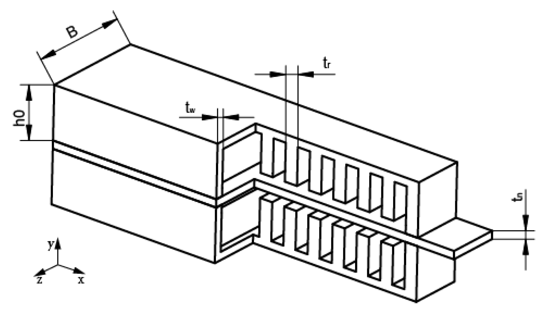
The dimension of the soft actuator can be shown in
Figure 1.
B is the width of the chamber,
is the height of the chamber after inflation,
is the thickness of the neutral layer,
is the thickness of the chamber, and
is the thickness of the rib.
For analytical purposes, the static moment study is carried out with the end of the neutral layer of the actuator. The driving force comes from the pressure in the chambers, and the torque produced by it can be expressed as
where
p is the pressure in the inflated side of the actuator, and
y is the direction shown in
Figure 1. A resistive moment
is generated in the neutral layer during the bending motion of the actuator. It can be presented as
where
E is the Young modulus of ABS,
I is the moment of inertia about
z-axis of the neutral layer.
is the bending angle of the actuator, and
L is the length of the actuator. The ABS plate has a Young’s modulus of 2 GPa and a Poisson ratio of 0.395, and
I can be calculated as
In addition, the tensile, compressive and shear stresses are generated by the deformation of the actuator. The circumferential stress of the actuator’s upper wall on the inflated side is denoted by
, the circumferential stress of the actuator’s sidewall on the inflated side is denoted by
, the compressive stress of the upper wall on the uninflated side is denoted by
, and the compressive stress of the side wall on the uninflated side is denoted by
. They can induce moments
,
,
and
, respectively. These moments can be presented as
The derivation process for all these moments can be found in our previous work on the static analysis [
11]. These moments, as well as
, prevent the soft pneumatic actuator from bending. These moments are defined as the moment generated by the internal force of the actuator. Then the
can be presented as
2.2. Dynamic Moment
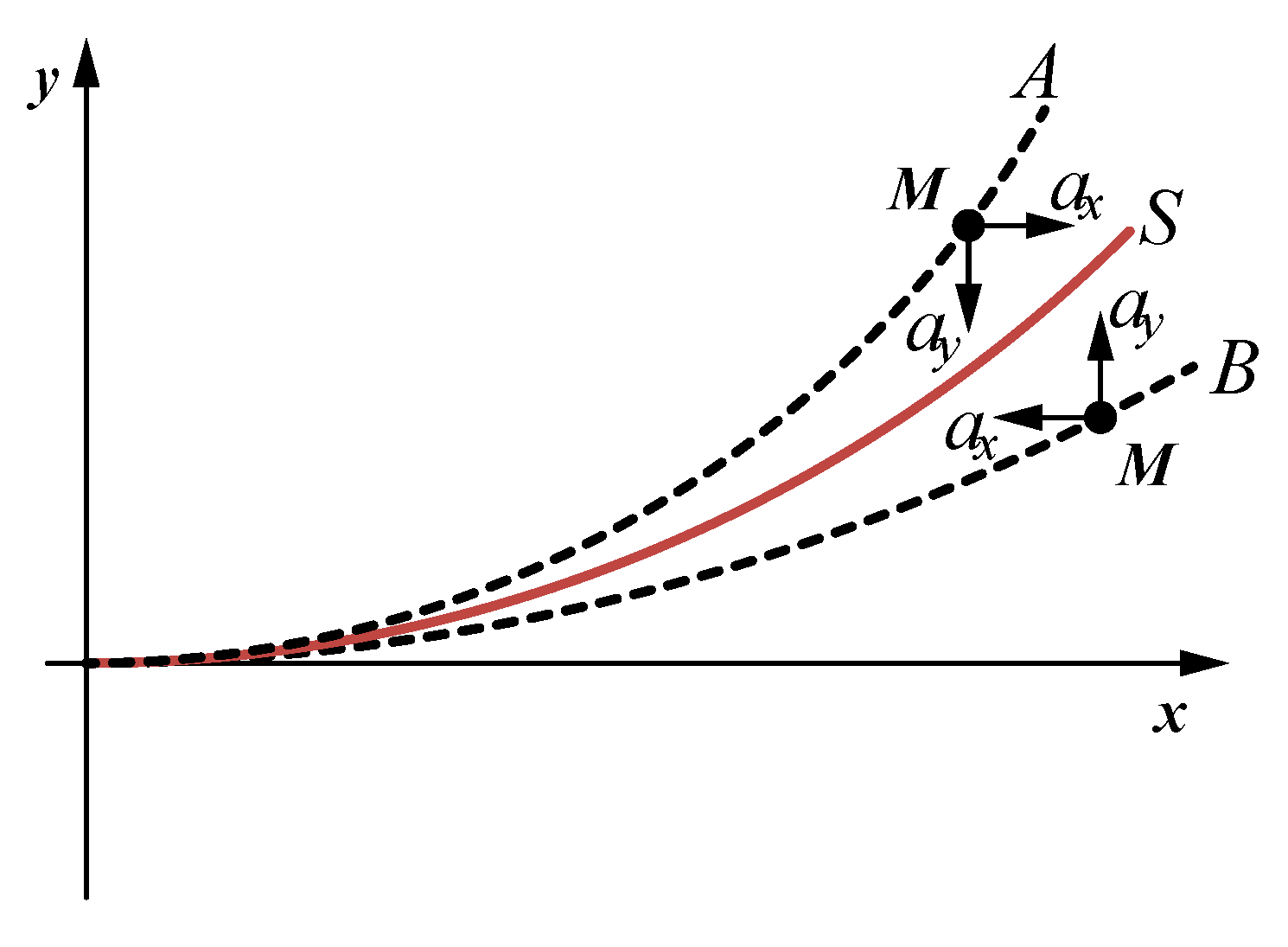
Based on the analysis of static moments, the dynamic moment balancing study is also carried out with the end of the neutral layer of the actuator. The moment of inertia, that is , consists of two moments, the rotational moment and the bending moment.
Assume that the static equilibrium position of the neutral layer of the actuator under the pressure p condition is
S.
A and
B are the two transient positions of the actuator during the motion when the pressure in the chambers is p, respectively. The acceleration of the mass point
M generated by the inertia force and its direction are shown in
Figure 2.
Then the bending moment generated by the inertia force can be presented as
where
is the bending moment,
is the mass of the mass point,
and
are the accelerations of the mass point, and
and
are the projections of the distance from the mass point to
O on the
x and
y axes.
If the length of the arc from the point in the
Figure 2 to
O is
r, the accelerations
and
can be presented as
Since the actuator itself is a symmetrical structure, the center of mass of the whole actuator is on the neutral layer. In order to simplify the calculation, the height change on the inflatable side and the mass shift due to shear deformation are ignored. The form of mass distribution of the actuator is simplified to a distribution along the midline of the constrained layer. It can be expressed by the line density. The density of the actuator is different at the chamber and ribbed positions, so using
and
denotes the linear density at the air cavity and rib plate, respectively.
Then, the bending moment can be obtained by integrating Equation (
10) over the length. Due to the density being different at the chamber and ribbed positions, the integrations are performed at different positions and finally summed.
where
N is the number of the chambers.
From the density distribution, it can also be concluded that the rotational moment of the actuator differs for different positions on the neutral layer with respect to the rotation axis. They are expressed as
and
.
Assume that the distance from a mass point of the actuator to the origin is
r. When the actuator is bent to
, the angular velocity of each point of the actuator is
, and the angular acceleration is
. By integrating the rotational inertia of the mass point over the entire length of the actuator, the rotational moment of the actuator can be expressed
The final dynamic equilibrium equation can be obtained by substituting the Equations (
2), (
6), (
10) and (
12) into Equation (
1), and the state of motion of the actuator can be obtained by solving this equation.
2.3. Compensation and Solution of the Dynamic Equilibrium Equation
Although the dynamic equilibrium equation has been established, this equation is very complex and difficult to solve. The equilibrium equation can be expanded to obtain the following form
where
and
are the function with respect to
;
C is a constant, and
is a function with respect to
p. In this equation, the expression for the coefficient of the
term is more complex, mainly due to the
and
functions. In order to facilitate the solution and improve the computational efficiency, it is necessary to make appropriate simplifications to the equation. Taylor expansions are performed for the
and
functions in Equation (
8), respectively, and the fourth order terms are retained. The dynamic equilibrium equation is simplified. This equation can be solved with the Runge–Kutta methods.
By solving this differential equation, it is shown that the process of motion solved by this model is oscillatory and cannot eventually reach the equilibrium state. This is mainly because the damping of the system is not considered, so the damping of the model needs to be compensated. The compensation is performed by adding a
term to the dynamic equilibrium equation. Due to the material properties, the movement of the actuator causes a change in the mass distribution. However, the mass distribution of the actuator is simplified to a distribution along the midline of the constrained layer, which is expressed by the line density. This can lead to errors in the dynamic moment calculation, so the changes in the mass distribution need to be compensated.
is added into the dynamic equilibrium equation. The equilibrium equation after adding compensation can expressed as
The
can be presented as
, and the
can be presented as
.
4. Results and Discussion
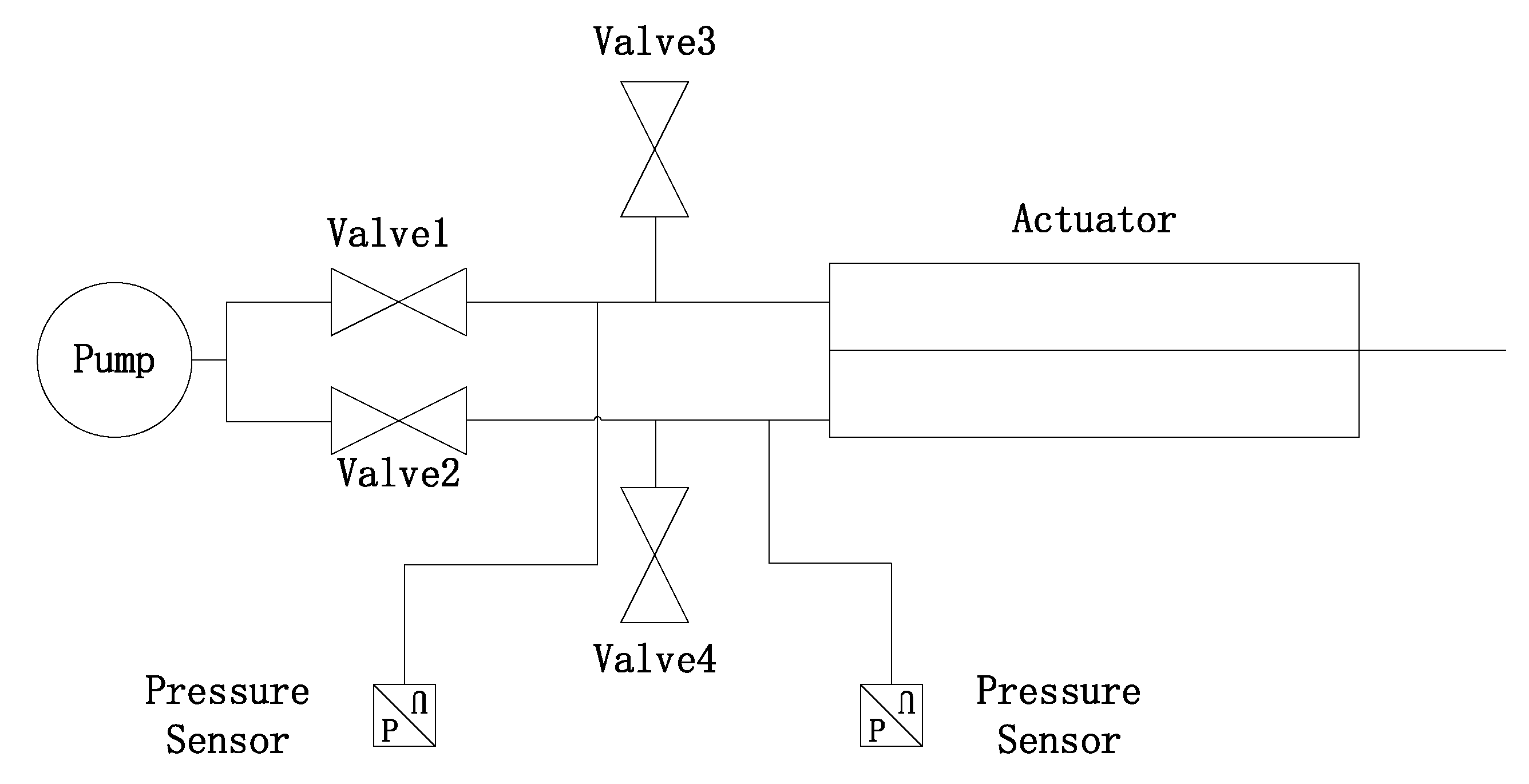
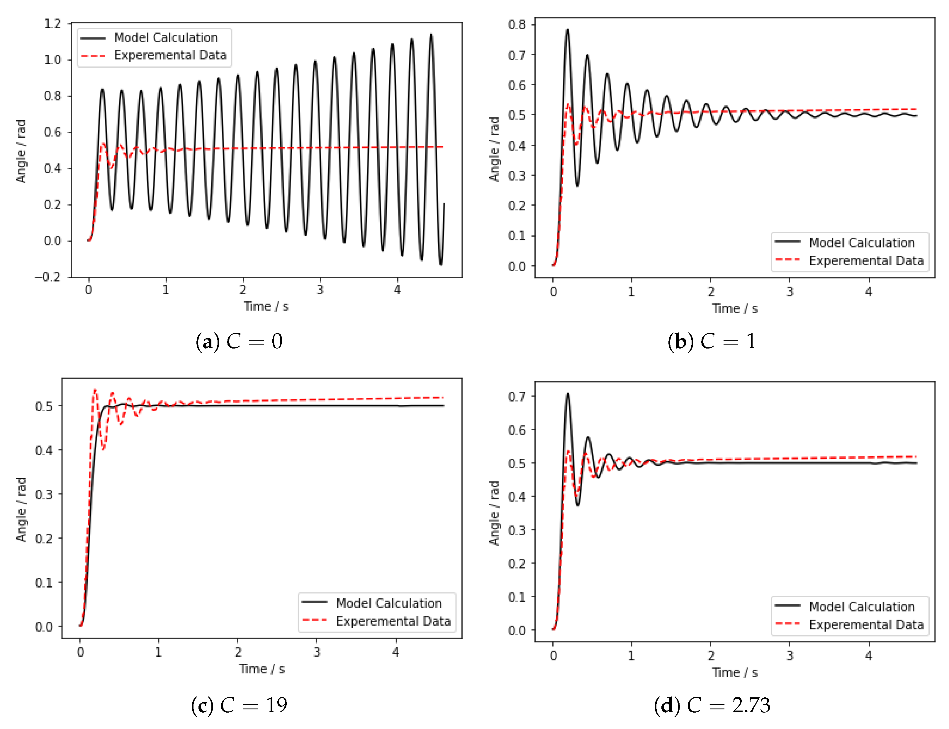
In the experiment, we inflate the chambers to 20 kPa on one side of the actuator and hold it, and the actuator bends to one side to reach the equilibrium position after several oscillations. According to the experimental conditions, the results by solving the dynamic equilibrium equation of the actuator are shown in
Figure 5. In order to verify the compensation effect of the model, the results for different damping compensation were calculated separately, and the results were compared with the experimental data.
In
Figure 5a, damping compensation is not performed, and it can be seen that the calculated motion curve does not converge, which also indirectly indicates that the system will oscillate without considering damping in the proposed dynamic model.
Figure 5b–d shows compensated damping. The motion curve converges after damping compensation. As
C increases, the system changes from an underdamped state to an overdamped state, and the number of system oscillations is directly related to the different damping compensation. Its final equilibrium position remains consistent with the experimental results regardless of how the system oscillates. This also proves the correctness of the static part of the proposed model. From the results, it can be seen that
Figure 5b is the underdamped state,
Figure 5c is the over-damped state, and
Figure 5d shows the optimal compensation coefficient, the number of its oscillations is basically consistent with the experimental data. It can be seen that there is a small error between the experimental data and the calculated results after the actuator reaches the equilibrium position in the figure. This is due to the drift of the gyroscope that measures the angle, i.e., the angle shows a small linear increase with time. This phenomenon has little effect on the measurement results.
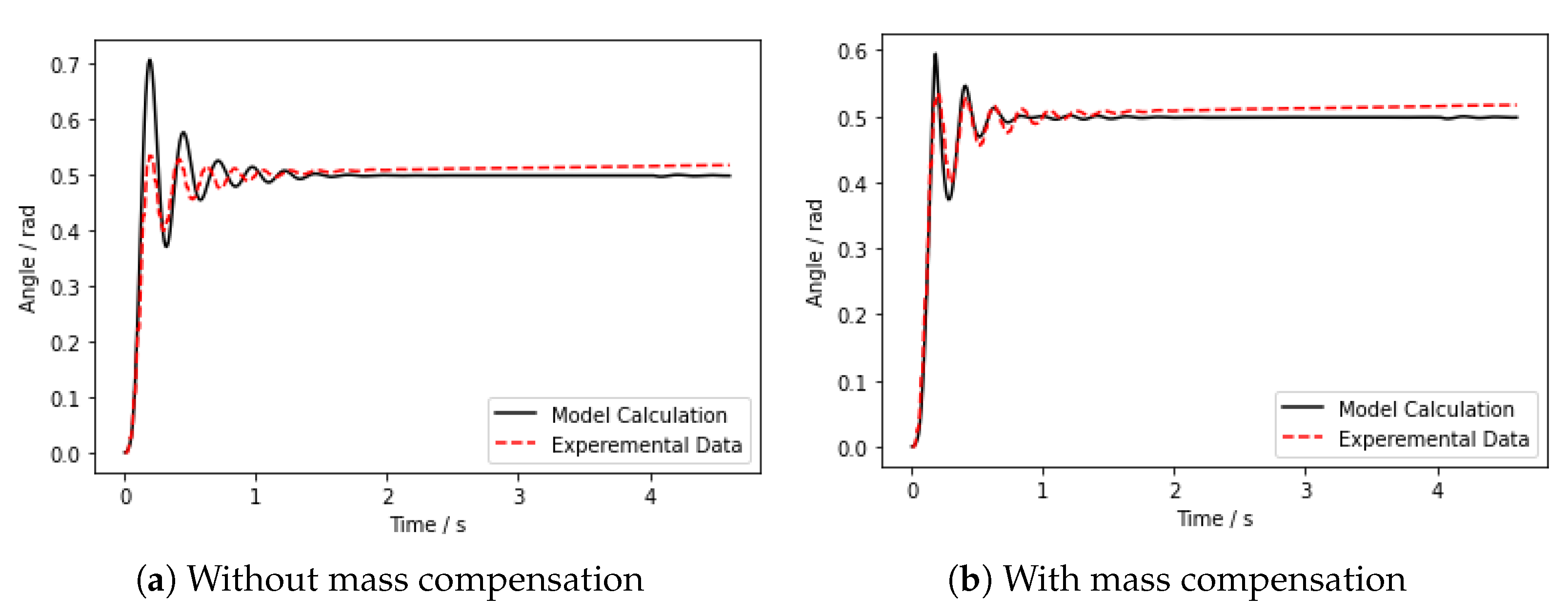
With the damping compensation, the number of system oscillations is generally consistent with the experiment, but the frequency of oscillation still has an error. Therefore, it is necessary to compensate for the mass, which is also explained in the previous section.
Figure 6 shows the comparison of the results of mass compensation.
Figure 6a shows that the frequency of oscillation is much different from the experimental data without compensation, while
Figure 6b shows that the frequency of oscillation is generally the same as the experimental data after adding mass compensation. In
Figure 6b, we can see that although the error of the model becomes smaller after compensation, there is still a little overshoot, which is caused by the hysteresis of the pneumatic circuit, and the actual response is smaller than the result calculated by the model. The results show that the proposed dynamic model can describe the motion process of this bi-directional pneumatic actuator effectively.
5. Conclusions
This paper proposed a dynamic modeling method for a bi-directional pneumatic actuator. The method utilizes D’Alembert’s principle and proposes a dynamic model of the actuator based on the static model. The errors resulting from the proposed dynamic equilibrium equation are analyzed, and a compensation method for the dynamic equilibrium equation is proposed. The solution process of the equation is also analyzed, and the equation can be calculated very quickly by using the Runge–Kutta method. According to the calculating tests, solving the model can be controlled within 1ms, so the actual control frequency can reach 1khz, which can meet the requirements of real-time control. At the end of this paper, the bi-directional motion experiments are performed for validating the proposed dynamic model, and the experimental results prove that the model still has a good accuracy. This model will also be applied to the actuator trajectory tracking control in our future work.

