Abstract
The variable stiffness exosuit has great potential for human augmentation and medical applications. However, the model of the variable stiffness mechanism in exosuits is far from satisfactory for the accurate prediction and control of friction force. This paper presents a friction prediction model of a variable stiffness lower limb exosuit, verifies its prediction performance, and identifies its applicability. The friction force model was established by the Coulomb friction hypothesis. The equivalent coefficient, which is the core parameter of the model, was determined based on friction and squeezing force data obtained by tests and an ANSYS simulation. Experiments show that the prediction error of the proposed model can reach 15% with a proper structural dimension change constraint. The friction force control test showed that the achieved model can shorten the settling time of the step response by 26% and eliminate the steady-state error. Verifications indicate that the proposed method can provide guidance to the modeling of other friction/stiffness structures, especially friction-based wearable robot structure models and predictions.
1. Introduction
Wearable robots, such as exoskeletons and soft exosuits, have received a considerable amount of attention in recent decades due to their significant potential for human function augmentation, rehabilitation training, and missing limb replacement [1]. As such, these robots are widely used in the military, medical, and industrial fields. Most exoskeletons made of rigid materials and joints have a high level of stiffness, accurate movement, and effective control. However, they are usually heavy and bulky [2,3,4,5]. In contrast, soft exosuits made of soft materials and mechanisms are light and compliant and exhibit better portability and human interaction flexibility. However, in some cases, such as the rehabilitation training of apoplectic patients [6] and human function augmentation of industrial workers [7], wearable robots require a stable support or additional joint buffer. Therefore, the development of variable stiffness wearable robots, particularly soft exosuits, is of great importance [8,9,10].
According to the realization principle of variable stiffness, wearable robots can be classified into three types: functional material-based [11,12,13,14,15,16,17,18], vacuum-based [19,20,21,22,23,24,25,26,27], and friction-based [28,29,30]. In particular, functional material-based type robots have obvious advantages in terms of volume and weight, and a shape memory alloy (SMA) is the most frequently employed functional material in the variable stiffness structure design [11,12]. Liu et al. [13] proposed a soft gripper with variable stiffness based on an SMA, which could grasp objects with a low level of stiffness and hold objects robustly with a high level of stiffness and a high degree of compliance. Experiments demonstrated that the stiffness of a single finger could be enhanced 18-fold. Another SMA-based soft gripper with variable stiffness was presented by Wang et al. [14]. By introducing the variable stiffness mechanism, the maximum grasping force increased. Yin et al. [15] constructed a fiber array muscle for a soft finger with variable stiffness by combining a composite fiber and an SMA. This model had good adaptability, a reduced sectional area, a compact structure, and a balance between large deformations and high loads in actuating. The shape memory polymer (SMP) is another functional material that is frequently applied to the variable stiffness structure design [16]. Yang et al. [17] designed novel soft robotic fingers operating SMPs to vary the stiffness. Variable stiffness and position feedback were both achieved through 3D printing of the SMP material. Chenal et al. [18] designed a variable stiffness fabric made from SMP and SMA. A soft finger joint exosuit made from the fabric was able to keep the fingers in the required position or allow the finger joints to move, as demonstrated in experiments. Thus, although the functional material-based type robot shows unique advantages, such as lightness and compliance [15,18], it has shortcomings, such as a long response time and low stiffness range, and still needs to be improved [12,17].
The emergence of a vacuum-based jamming mechanism provides an alternative for achieving variable stiffness in wearable robots [19]. Vacuum-based jamming can be categorized into two types: granular [20,21] and layer jamming [22,23,24,25,26,27]. Choi et al. [20] proposed a soft wearable robot for wrist support with a variable stiffness mechanism based on granular jamming. The maximum support force and the variable stiffness response time reached 19 N and 2 s, respectively. Hauser et al. [21] constructed an obedient and soft wearable robot (JammJoint) by applying granular jamming to vary the stiffness. It is noteworthy that the JammJoint demonstrated excellent portability and automation. However, the maximum bending torque in the experiments was only 1.6 Nm, making it difficult to support and buffer human knee joint motion. In contrast, a variable stiffness structure based on layer jamming has also been investigated by many researchers [22,23,24,25]. A variable stiffness exosuit based on layer jamming was proposed by Ibrahimi et al. [26], where the exosuit was utilized to maintain a supportive function and improve the comfort of the patients while sitting. A novel, soft, and multi-degree freedom layer jamming mechanism was proposed by Choi et al. [27]. In this model, variable stiffness could be achieved, and a large resisting force could be yielded in multiple directions. A higher stiffness and output force were achieved by layer jamming rather than granular jamming [26,27]. However, the variable stiffness structures based on layer jamming also tended to increase the volume and weight of soft exosuits and make the stiffness control more difficult [27].
Functional material-based and vacuum-based robots have difficulty in achieving a wide range of stiffness changes through a quick response using a light and compact mechanism, thus limiting their applications in most dynamic and heavy-duty situations, such as the lower limb exosuit [17,20]. Compared with these types of models, the friction-based type variable stiffness robot exhibits a natural superiority in terms of its controllable range and response time [28,29,30]. Miller-Jackson et al. [28] proposed a variable stiffness method based on friction caused by tubular inflation. They offered a new way to design exosuits for meeting heavy-duty tasks, such as joint motion buffering and weight bearing. Li et al. [29] presented a variable stiffness manipulator that could adjust the stiffness by changing the level of friction between the strips and the honeycomb core. A novel friction-based variable stiffness lower limb exosuit was designed by Xie et al. [30]. This has wide stiffness variation, a simple structure, and stiffness control, and can carry out locking and buffering for the motions of the human knee joint. However, in terms of friction-based variable stiffness structures, there is still no reasonable computation model for friction/stiffness prediction [28,30]. As friction/stiffness characteristics rely heavily on experimentation, accurate control of friction/stiffness requires a massive amount of experimental data, which is not always possible. Thus, the establishment and verification of prediction models of friction-based variable stiffness structures are of great importance.
In this study, a friction-based prediction model of a variable stiffness lower limb exosuit is presented, its predictive performance is validated, and its applicability is determined. The study is presented as follows: the working principle used for the variable stiffness structure is first introduced. Based on Coulomb’s friction law, we then describe the building of a friction model of the structure and the obtainment of material parameters through several air tube inflation experiments. Based on the model, the equivalent coefficient for friction prediction is determined by ANSYS simulations and several friction tests. Finally, the prediction and control performances are evaluated, and its applicability is identified through experiments.
The contribution and features of this study include the following: (1) in the friction prediction model, the equivalent coefficient is determined by ANSYS simulations, as well as experimental friction data, which contributes to the prediction of the semi-physical model. (2) A set of experiments is conducted, verifying the prediction performance and identifying the applicability of the model. Experimental results show that the model has a good prediction performance, indicating that the proposed method can provide guidance in terms of the design, modeling, and control of other friction-based variable stiffness structures, especially friction-based wearable robot structures.
2. Working Principle of Variable-Stiffness Structure
Figure 1 shows the overall structure and worn state of the soft exosuit. In terms of driving function, if one of the driving wires is pulled back in the middle part, this exosuit will assist in the bending or stretching movement of the knee joint. The driving wires made of steel cable are activated by air cylinders. Two brackets are positioned on the front of each cylinder to limit the displacement of the outer sheaths and transmit the force of the cylinders. Thus, driving wires enable the pulling force to be transmitted to the shank. In addition, the outer sheaths can also guide the driving wires. Air cylinders can be controlled by two two-position, three-way solenoid valves to alter the moving direction. These valves act in accordance with the signal from the controller, which is beneficial for controlling the movement of this exosuit. For the stiffness adjusting function, two air tubes made of silicon rubber are mounted, along with the two driving wires in two separate through-holes in the rigid part fixed on the thigh. When the air tubes are inflated by air pressure, the driving wires are squeezed against the hole wall, which leads to an increase in friction on the driving wires by the inner hole wall as well as by air tubes. When the air tubes are not inflated, the driving wires move freely, and the joint bending or stretching is unrestricted.
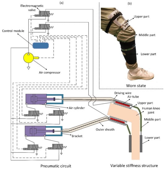
Figure 1.
(a) Pneumatic circuit and structure diagram; (b) Worn state of the exosuit.
Figure 2 shows the process of achieving variable stiffness. Only one side of the variable stiffness structure fixed with the human knee joint is displayed here. In the free state, the air tube is not inflated, and the joint moves freely; in the friction state, the air tube is inflated, which squeezes the driving wire and hinders its movement. In other words, the joint bending will lead to a friction moment caused by this friction force. The magnitude of this friction moment can be controlled by varying the inflation pressure of the air tube, which forms the core of the variable stiffness. The relationship between the friction force and the moment can be achieved easily by , where is the friction moment, is the friction force, and is the radius of curvature of the driving wire arc, as shown in Figure 2b. This shows that the relationship between the friction moment and friction force is linear on the condition that the value of is constant. However, when this exosuit is in working condition, the value of will change slightly, a process that is uncontrollable. Using the supporting materials between the steel cable and the leg, the change in can be minimized. Therefore, the value of is assumed to be constant in the analysis. The core of the prediction model is the modeling of the friction force acting on the driving wire. Obviously, the inflation pressure of the air tube determines this friction force. Thus, investing the relationship between the friction force and inflation pressure is the main task for establishing the friction prediction model.
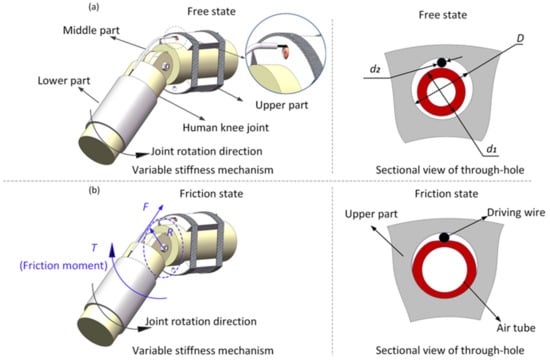
Figure 2.
Detailed view of the variable stiffness structure in (a) the free state and (b) the friction state.
3. Theoretical Model of Driving Wire Friction
It can be seen from the working principle of the variable stiffness structure that the friction force exerted by both the air tube and inner wall of the hole on the driving wire is the main parameter that we are concerned with in the friction/locking state. However, as the friction force is applied simultaneously by both the air tube and inner wall of the hole, it cannot be analyzed separately. In addition, owing to the small hole diameter of 10 mm, the squeezing force cannot be measured directly. For the abovementioned reasons, a prediction model of this friction force is necessary for good stiffness control and the structural design of the exosuit.
3.1. Modeling Analysis
With reference to Coulomb’s friction law, we hypothesize that the total friction force is proportional to the squeezing force, and the constant of proportionality is defined as the equivalent coefficient. Thus, the following equation can be obtained:
where is the equivalent coefficient of the model, is the squeezing force exerted by the air tube against the driving wire, is the inflation pressure, and represents a certain relationship between and , which can be investigated by ANSYS simulations (Ansys Inc., Pittsburgh, PA, USA). In Equation (1), is the unknown variable. Therefore, it is reasonable to combine the squeezing force determined by ANSYS simulations with the tested friction force to determine the value of . To obtain the friction force, an experimental platform was built, as shown in Figure 3. As for the squeezing force, the ANSYS simulation is an easy and efficient method compared to any direct measurement method considering the narrow diameter of the hole.
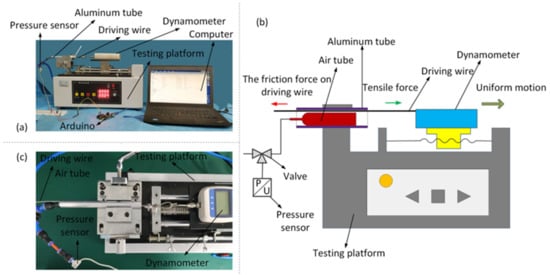
Figure 3.
(a) Testing platform to measure the friction force; (b) schematic of the testing platform; (c) local view of the friction force experiment.
3.2. Friction Experiments
The platform for testing the friction force is shown in Figure 3a. Because the exosuit was too large to be mounted on the testing platform, in order to vary the diameter of the hole rapidly with a reasonable cost, friction tests were conducted using aluminum tubes with the same material properties and inner hole wall roughness as those of the upper part of the exosuit. The aluminum tube was fixed on the testing platform, and the air tube was placed inside it along with the driving wire, as illustrated in Figure 3b. During testing, the air tube was first inflated, and the driving wire was then pulled to the right at a constant speed. Additionally, the friction force and inflation pressure values were measured using a dynamometer and pressure sensor and recorded by the computer.
The results of the friction experiments are shown in Figure 4. The curve represents the results when is 10 mm, is 8.3 mm, and is 1.6 mm, and the definitions of these parameters are shown in Figure 2a. This set of structural parameters is defined as the base group, which was the initial group employed to determine the equivalent coefficient in the prediction model. In Figure 4, is shown that the friction force increased almost linearly with an increasing inflation pressure. The maximum friction force reached 180.49 N when the inflation pressure was 0.6 MPa. It is known that when the tested radius was 0.10 m, the maximum friction moment obtained was 18.05 Nm, which indicates that the lower limb exosuit achieves a wide range of stiffness. This exosuit is capable of performing heavy-duty tasks, such as the buffering and locking motion of the knee joint.
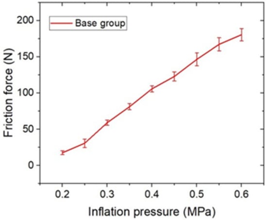
Figure 4.
Results of friction experiments.
3.3. Estimation of the Air Tube Material Parameters
To obtain the relationship between the inflation pressure and squeezing force, ANSYS simulations must be conducted. However, the air tube material, which is a type of silicon rubber, should first be studied. The silicon rubber used for air tube fabrication is one type of a super-elastic material, whose mechanical deformation behavior is nonlinear. A two-parameter Mooney–Rivlin model, which can simulate almost all silicon rubber materials, was utilized to build a constitutive equation for air tube deformations. This can also be applied in the case of 100–150% material deformation. Thus, the squeezing force can be calculated using ANSYS simulations with this model. The strain energy equation is as follows:
where is the strain energy density function, and are material parameters of silicon rubber, and are the first and second skew invariants of the left Cauchy–Green deformation tensor, and is the volume ratio. Commonly, the values of and can be calculated using the following empirical formula [31]:
where is the elastic modulus and is the shore hardness value of silicone rubber. This indicates that the elastic modulus can be determined by the shore hardness value of silicone rubber.
where is the shear modulus. This describes the relationship between the shear modulus and the elastic modulus of silicon rubber.
where is the material incompressible constant, and is the Poisson’s ratio. The parameters in Equations (3)–(6) were used in ANSYS simulations.
Equations (3)–(6) suggest that if the shore hardness value of silicone rubber is known, other material parameters can also be determined. Therefore, the air tube inflation experiments were designed to obtain the Shore hardness. Figure 5 shows the test circuit and results of the air tube inflation experiments.
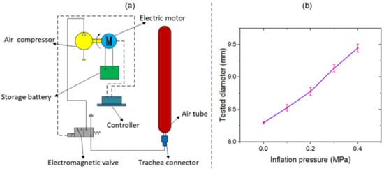
Figure 5.
(a) Test circuit of the inflation experiments; (b) results from the inflation experiments.
The shore hardness value of silicone rubber was estimated based on the bisection method and experimental verification. The bisection method is a highly efficient, accurate, and easy means of estimating parameters. The shore hardness range of silicon rubber in this study was found to be 60–70, and this varied slightly with the variation in material composition. According to the bisection method, the shore hardness values of the air tube were first assumed to be 60, 65, and 70. These parameters were introduced into Equations (3)–(6), and the diameters of the air tube at different inflation pressures were obtained by ANSYS simulations. The test data obtained by varying the diameter with pressure are shown in Figure 5b. A comparison between the simulations and the tested results is presented in Table 1. The average error, which represents the average absolute deviation between the simulated diameter and the tested diameter, was defined as the stopping criterion for the bisection method. If the average error was less than 0.50%, the bisection was stopped. Based on the results for the average error, the actual hardness was between 60 and 65, but both average errors were larger than 0.50%. Then, the hardness value was assumed to be 62.5, and the calculated average error was 0.46%, which satisfied the stopping criterion. Finally, the shore hardness value of silicone rubber was determined to be 62.5.

Table 1.
Diameters with different shore hardness values.
After the shore hardness value of the air tube was determined, the corresponding material parameters were calculated using Equations (3)–(6), as presented in Table 2. These material parameters acted as the basis for a squeezing force simulation using ANSYS, which was done later.
Table 2.
Material parameters of the air tube.
3.4. Squeezing Force Simulation
The plane strain problem analysis method was used for ANSYS simulations, as the air tube diameter was about 8.3 mm and its length was about 116 mm, meaning that the axial dimension was much larger than the radial dimension. The model was solved, and the squeezing force was calculated using ANSYS simulations, as shown in Figure 6.
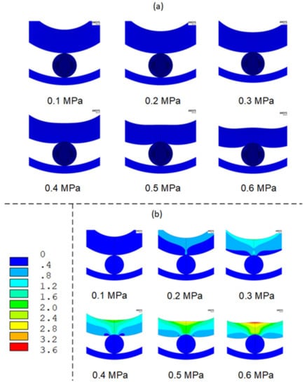
Figure 6.
(a) Air tube deformation simulations; (b) squeezing force simulations.
Figure 6a shows the air tube deformation at different inflation pressures. It was found that, with an increase in the inflation pressure, the deformation became more and more evident, and the contact surface between the air tube and the driving wire became larger. Figure 6b shows that the internal air tube stress became larger as the inflation pressure increased, and this was mainly concentrated in an area vertical to the contact surface. As shown in Figure 7, the squeezing force, which represents the vertical component of the contact force between the air tube and driving wire, was obtained by post-processing with ANSYS software. Figure 7 shows the variation in the squeezing force versus the inflation pressure.
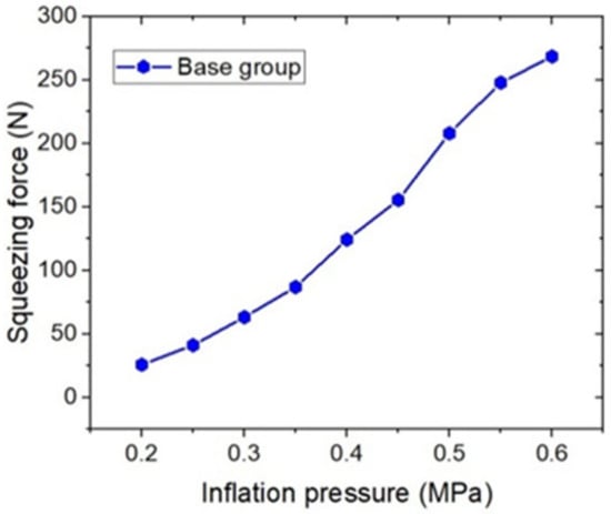
Figure 7.
Squeezing force obtained by ANSYS simulation.
The structural parameters of the base group used in the ANSYS simulations and shown in Figure 7 are the same as those shown in Figure 4. It can be seen that the squeezing force varied almost linearly. When the inflation pressure was 0.6 MPa, the squeezing force reached a maximum value of 268.55 N. However, compared with the friction force variation shown in Figure 4, the nonlinear variation of the squeezing force was more evident.
3.5. Determination of the Equivalent Coefficient
The least-squares method, which has the advantages of good accuracy and high calculation efficiency, was utilized to identify the equivalent coefficient of the model. The equation used for the least-squares method was as follows:
where denotes the square sum of error, denotes the square error, denotes the sampling number, and denotes the tested friction force. Using this method, an equivalent coefficient of 0.7168 was determined with a relative error of 10.68%.
According to the prediction model, the squeezing force should first be obtained by ANSYS simulations to predict the friction force for dimensions other than those used in the base group, and the predicted friction force can be calculated by Equation (1) using the obtained equivalent coefficient. This acquired model applies to two situations: (1) after some large structural dimension other than those used in the base group is designed, the variation law of friction force and its maximum value can be obtained by the prediction model, which determines whether the structural dimensions have been modified and (2) for friction force feedback control. As for dimensions other than the base group, the squeezing force can be obtained by ANSYS simulations. The cubic curve can be fitted to describe the relationship between the squeezing force and inflation pressure. Using Equation (1), the relation between the friction force and inflation pressure can be deduced, which can be applied for feedback control.
4. Verification and Identification of Applicability
After the friction model was established based on the base group, the prediction performance had to be verified, and the applicability needed to be identified by varying the structural dimensions. As shown in Table 3, three groups of experiments were conducted. In the first group, the dimensional values of , , and were proportionally changed with those of the base group (since the driving wire diameter had to be changed discretely due to the use of steel cable products, the deviation in the dimensions was less than 10%). In the second group, the values of , , and were changed proportionally to those of the base group, and a deviation in the range of 10–20% was used. In the third group, the values of , , and were proportionally changed to those of the base group with a deviation of more than 20%.
Table 3.
Pre-set parameters for different experimental groups.
Figure 8 shows the prediction performance of the first group. Figure 8a,b show the results of tests 2 and 3, respectively. The left side shows the predicted friction force (black curve) and tested friction force (red curve); the right side shows the relative error results. The maximum relative errors in tests 1 and 2 were found to be −12.00% and −10.16%, respectively, which indicates that this model has a good prediction performance when the dimensions change proportionally with a deviation of less than 10%.
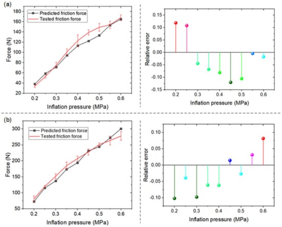
Figure 8.
Results of (a) test 2 and (b) test 3.
Figure 9 shows the prediction performance of the second group. Figure 9a,b show the results of tests 4 and 5, respectively. The maximum relative errors in tests 4 and 5 were −24.96% and 12.45%, respectively, which indicates that this model has a lesser prediction performance than the previous case when the dimensions proportionally change with a deviation in the range of 10–20%.
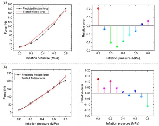
Figure 9.
Results of (a) test 4 and (b) test 5.
Figure 10 shows the prediction performance of the third group. Figure 10a,b show the results of tests 6 and 7. The prediction model showed an evident deviation across the whole range. The maximum relative errors in tests 6 and 7 were 188.64% and −92.36%, respectively, which indicates that this model does not have an acceptable prediction performance when the dimensions change proportionally with a deviation more than 20%.
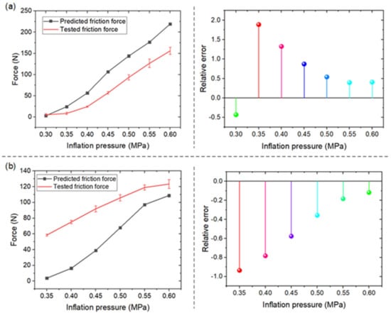
Figure 10.
Results of (a) test 6 and (b) test 7.
The above analysis indicates that the prediction error of the friction force increased as the proportional deviation from the structural base dimensions increased. When the maximum relative deviation was less than 10%, the prediction error was less than 15%. When the maximum relative deviation was in the interval of 10–20%, the prediction error was less than 25%. Thus, when the maximum relative deviation was less than 20%, the friction model had a satisfactory prediction performance. When the maximum relative deviation was more than 20%, the prediction error was more than 90%, which illustrates that the prediction model was not useful at all.
To further identify the applicability of the proposed model, the ANOVA method was applied to test the significance between the base group and other groups, in which the prediction error was treated as the dependent variable. The results are shown in Table 4.
Table 4.
ANOVA results.
As shown in Table 4, the p-values of tests 6 and 7 were less than 0.05, which indicates that compared with the base group, they were significantly different; thus, the friction prediction model is inapplicable when the dimension deviation of the structure is higher than 20%. However, for the other four groups, the p-values were greater than 0.05, meaning that the friction prediction model is applicable when the structural dimension deviation is within 15%.
The above friction prediction experiments show that the maximum friction, which occurred in test 3, reached 300 N, which means that, when the tested radius was 0.10 m, as shown in Figure 2b, this variable stiffness exosuit can provide a torque of 30 Nm to support the human body. This is enough to meet the torque requirements (0–40 Nm) of human knee joint movement [32]. This point suggests that the achieved model could help us to determine the dimensions of the variable stiffness structure at the pre-design stage.
5. Control System Based on the Model
By applying the friction model and PID control to build a closed-loop control system, the friction force can be controlled accurately and rapidly. For example, the structure used in test 5 was utilized to build a closed-loop control system based on the testing platform shown in Figure 3. The fitted cubic curve of the squeezing force variation with the inflation pressure is shown in Figure 11.
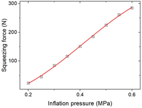
Figure 11.
Fitted cubic curve.
As shown in Figure 11, all data points were mainly located in the cubic curve. The squeezing force variation law, described by the cubic polynomial and R-square (COD), was found to be 0.999, which illustrates that the curve fitting performance was excellent. The equation is as follows:
According to Equation (1), the variation in friction force with the inflation pressure is as follows:
When a certain friction force is required, an inflation pressure value between 0.2 and 0.6 MPa can be determined. For the friction force of 54.40 N, the calculated inflation pressure is about 0.26 MPa. Thus, by combining Equation (9) with the PID control, closed-loop control systems can be built. As a classical control method, PID control can be applied widely in various systems, having adaptive performance for models with unknown parameters. It is obvious that three types of the traditional PID control method can be designed: PID control, PI control, and PD control. The performances of different control strategies are shown in Figure 12.
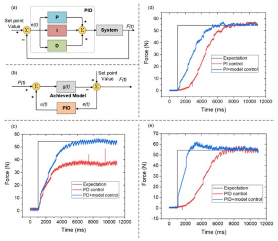
Figure 12.
(a) The PID control method schematic with and without the proposed model; (b) closed-loop control method; (c) PD control performance; (d) PI control performance; (e) PID control performance.
Figure 12a shows the principle of PID control. The friction force can be controlled only by the PID control method, which is as follows:
where is the error term, is the proportional term, is the integral term, is the derivative term, and is the feedback input value. , and can be determined by the experimental method.
Figure 12b shows the principle of the closed-loop control system, which applies PID to deal with the feedback error. is the relationship between the inflation pressure and friction force mapped on the time axis, as follows:
Figure 12c–e shows the application of the PD, PI, and PID control, in which the horizontal axis is time and the vertical axis is friction force. The black curve represents the expected performance; that is, a friction force of 54.40 N. The red curve shows the performance of the control method without the model, and the blue curve shows the performance of the control method with the model.
As shown in Figure 12c, pure PD control without the model would result in a steady-state error that cannot be eliminated. However, PD control with the model can eliminate the steady-state error, where the values of and are the same. The settling time of PD control with the model was about 4.41 s.
Figure 12d shows that, compared with the PI control, PI control with the model has a shorter settling time. The settling time of PI control was about 5.73 s, while the settling time of PI control with the model was about 4.20 s. The settling time was reduced by 26%.
Figure 12e shows that, compared with the PID control, PID control with the model could reduce the settling time. The settling time of PID control was about 6.17 s, while the settling time of PID control with the model was about 4.39 s. The settling time was reduced by 29%. For PI and PID control, the introduction of this model would reduce the settling time and the performances would be largely the same. For PD control, the introduction of this model would eliminate the steady-state error. The experimental results illustrate that PD/PI/PID control with the model could be applied.
The study of the control system showed that the friction model has the potential to control friction/stiffness and improve the response speed, contributing to its performance when providing locking and buffering protection for the human knee joint.
6. Discussion
The variable stiffness exosuit has a great potential for human augmentation and medical applications. Nevertheless, the model of the variable stiffness mechanism in exosuits is far from satisfactory in terms of the accurate prediction and control of the friction force. Thus, the establishment and verification of a prediction model of friction-based variable stiffness structures are of great importance. In this study, we established a friction prediction model of a lower limb exosuit with variable stiffness, verified its prediction performance, and identified its applicability. In the model establishment process, a Coulomb’s friction law hypothesis was employed, in which the equivalent coefficient was the core parameter to be determined. This coefficient was determined through the least-squares method using experimental friction force data as well as squeezing force data obtained by ANSYS simulations.
The least-squares method was used to determine the equivalent coefficient, which was 0.7168 with an average error of 10.68% for dimensions proportional to the base group. The acquired model can be used in two situations: (1) when a large structural dimension other than the base group is designed, the variation law of friction force can be obtained by the prediction model, which determines whether the structural dimensions are modified and (2) for friction force feedback control.
Our experiments demonstrate that the friction prediction model has satisfactory prediction performance, and the closed-loop control provided by this model exhibits a quick response. It is worth noting that the acquired model could be transferred to other systems. For example, in soft structures (TJH and TJB) proposed by Miller-Jackson et al. [28], the acquired model/method can be used to determine the friction coefficient between soft tubulars, which is beneficial for the precise control of joint bending. Additionally, in the reconfigurable variable stiffness manipulator presented by Li et al. [29], the friction coefficient between the strips and the honeycomb core should be analyzed to improve the prediction accuracy for the manipulator’s posture.
7. Conclusions
In this paper, a friction prediction model was proposed and verified, and its applicability was determined. The acquired model can provide guidance in the modeling of other friction/stiffness structures, particularly the modeling and prediction of friction-based wearable robot structures. Experiments and the ANOVA method demonstrated that the friction model has satisfactory prediction performance with a friction prediction error of less than 25% when the dimensions are proportionally varied with a deviation of less than 20%. The prediction error can reach 15% with a deviation of less than 10%. Friction force control tests showed that the model can shorten the settling time of the step response by 26% and eliminate the steady-state error.
In the future, we will further improve the model’s accuracy and explore its application in other friction-based variable stiffness applications. In addition, more investigations need to be conducted on the exosuit presented in this work to evaluate its performance in providing locking and buffering protection for the human knee joint.
Author Contributions
Conceptualization, J.L.; data curation and writing original draft, Z.M.; supervision, S.Z.; writing—review and editing, B.C. All authors have read and agreed to the published version of the manuscript.
Funding
This research was funded by the National Key R&D Program of China under Grant No. 2019YFB1311501, in part by National Natural Science Foundation of China under Grant No. 51905374 and in part by the Open Project Program of Tianjin Key Laboratory of Aerospace Intelligent Equipment Technology, Tianjin Institute of Aerospace Mechanical and Electrical Equipment under Grant No. TJWDZL2019KT007.
Conflicts of Interest
The authors declare no conflict of interest.
References
- Pons, J.L. Witnessing a wearables transition. Science 2019, 365, 636–637. [Google Scholar] [CrossRef] [PubMed]
- Jafari, A.; Tsagarakis, N.G.; Caldwell, D.G. AwAS-II: A new Actuator with Adjustable Stiffness based on the novel principle of adaptable pivot point and variable lever ratio. In Proceedings of the 2011 IEEE International Conference on Robotics and Automation, Shanghai, China, 9–13 May 2011. [Google Scholar]
- Liu, Y.; Guo, S.; Hirata, H.; Ishihara, H.; Tamiya, T. Development of a powered variable-stiffness exoskeleton device for elbow rehabilitation. Biomed. Microdevices 2018, 20, 64. [Google Scholar] [CrossRef]
- Tonietti, G.; Schiavi, R.; Bicchi, A. Design and Control of a Variable Stiffness Actuator for Safe and Fast Physical Hu-man/Robot Interaction. In Proceedings of the 2005 IEEE International Conference on Robotics and Automation, Barcelona, Spain, 18–22 April 2005. [Google Scholar]
- Wolf, S.; Hirzinger, G. A new variable stiffness design: Matching requirements of the next robot generation. In Proceedings of the 2008 IEEE International Conference on Robotics and Automation, Pasadena, CA, USA, 19–23 May 2008. [Google Scholar]
- Xu, G.Z.; Gao, X.; Chen, S.; Wang, Q.; Zhu, B.; Li, J.F. A novel approach for robot-assisted upper-limb rehabilitation: Pro-gressive resistance training as a paradigm. Int. J. Adv. Robot. Syst. 2017, 14, 1–12. [Google Scholar] [CrossRef]
- Chen, S.; Stevenson, D.T.; Yu, S.; Mioskowska, M.; Yi, J.A.F.T.; Su, H.; Trkov, M. Wearable Knee Assistive Devices for Kneeling Tasks in Construction. IEEE/ASME Trans. Mechatron. 2021. [Google Scholar] [CrossRef]
- Blanc, L.; Delchambre, A.; Lambert, P. Flexible Medical Devices: Review of Controllable Stiffness Solutions. Actuators 2017, 6, 23. [Google Scholar] [CrossRef] [Green Version]
- Manti, M.; Cacucciolo, V.; Cianchetti, M. Stiffening in Soft Robotics: A Review of the State of the Art. IEEE Robot. Autom. Mag. 2016, 23, 93–106. [Google Scholar] [CrossRef]
- Zhang, Y.; Lu, M. A review of recent advancements in soft and flexible robots for medical applications. Int. J. Med. Robot. 2014, 16, e2096. [Google Scholar] [CrossRef]
- McEvoy, M.A.; Correll, N. Shape-Changing Materials Using Variable Stiffness and Distributed Control. Soft Robot. 2018, 5, 737–747. [Google Scholar] [CrossRef] [PubMed]
- Rodrigue, H.; Wang, W.; Han, M.-W.; Kim, T.J.; Ahn, S.-H. An Overview of Shape Memory Alloy-Coupled Actuators and Robots. Soft Robot. 2017, 4, 3–15. [Google Scholar] [CrossRef]
- Liu, M.; Hao, L.; Zhang, W.; Zhao, Z. A novel design of shape-memory alloy-based soft robotic gripper with variable stiffness. Int. J. Adv. Robot. Syst. 2020, 17, 1–12. [Google Scholar] [CrossRef]
- Wang, W.; Ahn, S.-H. Shape Memory Alloy-Based Soft Gripper with Variable Stiffness for Compliant and Effective Grasping. Soft Robot. 2017, 4, 379–389. [Google Scholar] [CrossRef] [PubMed]
- Yin, H.; Tian, L.; Yang, G. Design of fibre array muscle for soft finger with variable stiffness based on nylon and shape memory alloy. Adv. Robot. 2020, 34, 599–609. [Google Scholar] [CrossRef]
- Rossiter, J.; Takashima, K.; Scarpa, F.; Walters, P.; Mukai, T. Shape memory polymer hexachiral auxetic structures with tunable stiffness. Smart Mater. Struct. 2014, 23, 045007. [Google Scholar] [CrossRef] [Green Version]
- Yang, Y.; Chen, Y.; Li, Y.; Wang, Z.; Li, Y. Novel Variable-Stiffness Robotic Fingers with Built-In Position Feedback. Soft Robot. 2017, 4, 338–352. [Google Scholar] [CrossRef]
- Chenal, T.P.; Case, J.C.; Paik, J.; Kramer, R.K. Variable stiffness fabrics with embedded shape memory materials for wearable applications. In Proceedings of the 2014 IEEE/RSJ International Conference on Intelligent Robots and Systems, Chicago, IL, USA, 14–18 September 2014. [Google Scholar]
- Trappe, V.; Prasad, V.; Cipelletti, L.; Segre, P.N.; Weitz, D.A. Jamming phase diagram for attractive particles. Nature 2001, 411, 772–775. [Google Scholar] [CrossRef] [PubMed]
- Choi, J.; Lee, D.-Y.; Eo, J.-H.; Park, Y.-J.; Cho, K.-J. Tendon-Driven Jamming Mechanism for Configurable Variable Stiffness. Soft Robot. 2020, 8, 109–118. [Google Scholar] [CrossRef] [PubMed]
- Hauser, S.; Robertson, M.; Ijspeert, A.J.; Paik, J. JammJoint: A Variable Stiffness Device Based on Granular Jamming for Wearable Joint Support. IEEE Robot. Autom. Lett. 2017, 2, 849–855. [Google Scholar] [CrossRef]
- Zhou, Y.; Headings, L.M.; Dapino, M.J. Discrete Layer Jamming for Variable Stiffness Co-Robot Arms. J. Mech. Robot. 2020, 12, 015001. [Google Scholar] [CrossRef]
- Mikol, C.; Su, H.-J. An Actively Controlled Variable Stiffness Structure via Layer Jamming and Pneumatic Actuation. In Proceedings of the 2019 International Conference on Robotics and Automation (ICRA), Montreal, QC, Canada, 20–24 May 2019. [Google Scholar]
- Mitsuda, T.; Gerling, G. Variable-stiffness Sheets Obtained using Fabric Jamming and their Applications in Force Displays. In Proceedings of the 2017 IEEE World Haptics Conference, Munich, Germany, 6–9 June 2017; IEEE: New York, NY, USA, 2017; pp. 364–369. [Google Scholar]
- Zeng, X.; Hurd, C.; Su, H.-J.; Song, S.; Wang, J. A parallel-guided compliant mechanism with variable stiffness based on layer jamming. Mech. Mach. Theory 2020, 148, 103791. [Google Scholar] [CrossRef]
- Ibrahimi, M.; Paternò, L.; Ricotti, L.; Menciassi, A. A Layer Jamming Actuator for Tunable Stiffness and Shape-Changing Devices. Soft Robot. 2020, 8, 85–96. [Google Scholar] [CrossRef]
- Choi, W.H.; Kim, S.; Lee, D.; Shin, D. Soft, Multi-DoF, Variable Stiffness Mechanism Using Layer Jamming for Wearable Robots. IEEE Robot. Autom. Lett. 2019, 4, 2539–2546. [Google Scholar] [CrossRef]
- Miller-Jackson, T.; Sun, Y.; Natividad, R.; Yeow, C.H. Tubular Jamming: A Variable Stiffening Method Toward High-Force Applications with Soft Robotic Components. Soft Robot. 2020, 7, 408. [Google Scholar] [CrossRef] [PubMed]
- Li, D.C.F.; Wang, Z.; Ouyang, B.; Liu, Y.-H. A Reconfigurable Variable Stiffness Manipulator by a Sliding Layer Mechanism. In Proceedings of the 2019 International Conference on Robotics and Automation (ICRA), Montreal, QC, Canada, 20–24 May 2019; IEEE: New York, NY, USA, 2019; pp. 3976–3982. [Google Scholar]
- Xie, D.; Liu, J.; Zuo, S. Pneumatic Flexible Exoskeleton with Variable Stiffness Based on Wire Driving and Clamping. In Proceedings of the 2019 IEEE 9th Annual International Conference on CYBER Technology in Automation, Control, and Intelligent Systems (CYBER), Suzhou, China, 29 July–2 August 2019. [Google Scholar]
- Zuo, L. Finite Element Analysis of Common Rubber Components Used in Locomotive and Vehicle. Master’s Thesis, Southwest Jiaotong University, Chengdu, China, 2008. [Google Scholar]
- Liu, Y. Research on the Cable-Pulley Underactuated Lower Limb Exoskeleton. Master’s Thesis, Harbin Institute of Technology, Harbin, China, 2018. [Google Scholar]
Publisher’s Note: MDPI stays neutral with regard to jurisdictional claims in published maps and institutional affiliations. |
© 2021 by the authors. Licensee MDPI, Basel, Switzerland. This article is an open access article distributed under the terms and conditions of the Creative Commons Attribution (CC BY) license (https://creativecommons.org/licenses/by/4.0/).