Article

Dynamic Parameter Estimation of Large Space Debris Based on Inertial and Visual Data Fusion

1
State Key Laboratory of Reliability and Intelligence of Electrical Equipment, Hebei University of Technology, Tianjin 300401, China
2
School of Mechanical Engineering, Hebei University of Technology, Tianjin 300130, China
3
Beijing Institute of Spacecraft System Engineering, Beijing 100094, China
*
Author to whom correspondence should be addressed.
Actuators 2021, 10(7), 149; https://doi.org/10.3390/act10070149
Submission received: 10 May 2021 / Revised: 13 June 2021 / Accepted: 22 June 2021 / Published: 2 July 2021
(This article belongs to the Special Issue Actuation for Space Applications)

Abstract

:
Most large space debris has large residual angular momentum, and the de-tumbling and capturing operation can easily cause instability and failure of tracking satellites. Therefore, it is necessary to perform real-time dynamic parameter identification of space debris prior to the imminent de-tumbling and capture operation, thus improving the efficiency and success of active debris removal (ADR) missions. A method for identifying dynamic parameters based on the fusion of visual and inertial data is proposed. To obtain the inertial data, the inertial measurement units (IMU) with light markers were fixed on the debris surface by space harpoon, which has been experimentally proven in space, and the binocular vision was placed at the front of a tracking satellite to obtain coordinates of the light markers. A novel method for denoising inertial data is proposed, which will eliminate the interference from the space environment. Furthermore, based on the denoised data and coordinates of the light markers, the mass-center location is estimated. The normalized angular momentum is calculated using the Euler–Poinsot motion characteristics, and all active debris removal parameters are determined. Simulations with Gaussian noise and experiments in the controlled laboratory have been conducted, the results indicate that this method can provide accurate dynamic parameters for the ADR mission.

Graphical Abstract

1. Introduction

As human space activities increase, the condition of space debris gradually deteriorates, and the probability of collision with spacecrafts in orbit gradually increases [1,2,3,4]. Among them, large space debris such as rocket upper stages will create a large number of new fragments after the collisions and disintegration, which seriously threatens the safety of orbiting spacecraft. Therefore, the active debris removal (ADR) mission, which include de-tumbling and capture operation, is necessary to carry out. Large space debris is mostly more than 2 m in size [5]. It is affected by the gravity of the earth, sunlight pressure, and residual angular momentum, and often presents the spin, nutation, and precession mixed motion at around 40 rpm [6]. So, the knowledge of large debris’ dynamic parameters and inertial properties is crucial for ADR mission.
For the estimation of three-axis tumbling debris’ dynamic parameters, the stereo-vision methods have been widely used. Tweddle et al. [7,8] proposed a method to estimate the dynamic parameters of non-cooperative targets based on binocular vision. In this method, aiming at the space proximity operation [9], the rotation of space debris was modeled by the Euler–Poinsot model, and the estimation of parameters was regarded as SLAM. The linear velocity, angular velocity, mass-center location, and normalized inertia tensor matrix were considered, and the factor graph method was used to establish the solution model. Finally, iSAM (incremental smoothing and mapping) system was used to acquire the corresponding motion and inertia parameters. The effectiveness of this method has been verified by space station experiments [10]. At the same time, Tweddle analyzed the observability of the binocular vision measurement method and concluded that when measuring the inertia tensor matrix, the rank of the observation matrix is one less than the number of variables. So, normalization is used to quantify inertia tensor. This normalization was also used by many visual measurement methods [11,12,13,14]. Setterfield et al. [11,12] described a procedure of estimating the inertial properties based on stereo vision, and also used Euler–Poinsot to model the rotation of space debris. By considering the relative magnitude of angular momentum and angular kinetic energy, as well as the relative situation of the principal moment of inertia, the motion was divided into seven forms, and two most common cases were considered. By analyzing the geometric properties of the polhode, the optimization equation was established to solve the estimation of the principal axes. The dynamic equation of Euler–Poinsot motion was analyzed and deduced, and the optimization of inertia ratio estimation was solved. Vincenzo Pesce et al. [13] regarded the relative position, attitude, velocity, angular velocity, and inertia ratio of space debris as state variables, and used a nonlinear state equation to model the dynamic characteristics of non-cooperative targets. He took the motion equation as a process model. The stereo-vision observation equation and Euler dynamic equation were regarded as the observation model. IEKF (iterated extended Kalman filter) was used for the above model. Numerical simulation showed that the method can quickly converge and showed good robustness. QIU et al. [14] proposed a two-step method to estimate the inertia ratio, attitude, angular velocity and the direction of angular momentum. The EKF (Extended Kalman Filter) was used, and numerical simulations were performed, which showed the accurate estimate. Radar, LIDAR and TOF cameras are also used for the identification of space debris dynamics parameters [15,16,17,18,19]. Bai et al. [15] creates a data-recording model for radar’s two-dimensional (2D) ISAR imaging of rotating objects, and the effectiveness of the algorithms is demonstrated by simulations. For the pose determination of uncooperative targets, Opromolla et al. [16] proposed a customized three dimensional template matching approach, which is used to obtain initial pose, and ICP algorithm is used for pose tracking. Numerical simulations verify the high accuracy and robustness of the method, but the real-time performance of the algorithm is not better than other algorithms and cannot meet the requirements of the ADR tasks. Based on radar data and time-frequency based signal processing, Ghio et al. [17] proposed an method that is used to estimate the geometrical and motion parameters of resident space objects located in the LEO region. Furthermore, the high accuracy and high real time performance of the method is demonstrated by simulation. Using the a K-band frequency-modulated continuous-wave radar data, Ghio et al. [18] identified the size and spin rate of the space objects, and the experimental results proved that the method can be effectively used for identifying spinning space debris characterization. In [19], Ghio et al. compared the methods relying on inverse radon transform for the estimation of the object’s rotation period.
The above methods are used for Phase I of proximity operation (The phases of the proximity operation are: I—Observing and Planning; II—Final Approaching; III—Impact and Capture; IV—Post-capturing stabilization [9]), that is, checking the target at a safe distance, obtaining information about the target, and planning the follow-up phase [11]. In this phase, there is no need for high accuracy, the visual method can achieve good results. However, in the subsequent phases, especially in Phase 3, which include ADR mission, the error of the visual method is unbearable. For example, in Pesce’s work [13], the convergence value of relative-position error is above 0.4 m. Therefore, the visual method is not suitable for the ADR mission. To solve the problem of Phase III, Qingliang Meng et al. [20] used binocular vision and a flexible rod with a force–moment sensor to identify the dynamic parameters of non-cooperative targets. In this method, the flexible rod carried by the tracking satellite was used to change the motion of the target, and the force–moment sensor at the end of the flexible rod was used to identify the contact force. The binocular vision was used to identify the changes of the target pose. Using the data, all inertia parameters of space debris, including the mass of space debris that could not be recognized by vision, were estimated. However, this method has some risks: when the target is larger than the tracking satellite, if the flexible rod was exerted on the hole of the target and cannot be pulled out in time, the detection satellite might be temporarily attached to the target, which will cause satellite instability or even loss of control.
To solve the shortcomings of existing methods, an inertial parameter estimation method of non-cooperative targets based on binocular vision and inertial measurement unit (IMU) fusion is proposed in this paper. This method combines the visualization of the visual method and the accuracy of inertial sensors’ measurement, can quickly and accurately estimate dynamic parameters of targets, and convert the parameters to the ADR coordinate system, which is beneficial to calculate direction and magnitude of de-tumbling and capture’s torque. This method refers to I.V.Belokonov’s work [21] in the use of IMU. I.V.Belokonov assumes that inertial units can be fixed on space debris using nanosatellites, regardless of how to launch and attach the nanosatellites to the debris surface, only the detection process is considered, and the following two hypotheses are made:
(a)
The mechanical connection of IMU is rigid;
(b)
Because the measurement time is very short, the perturbation moment has a minimal influence on the motion, and the influence is not considered.
In this paper, we also use the above assumption: the inertial unit can be attached to the surface of space debris using the space harpoon [22], which has successfully done space experiments. Because the IMUs are generally light, it does not bring too much difficulty to the attachment. In the next section, we will discuss the feasibility of space harpoon attachment, but as this paper is mainly concerned with the subsequent identification of the dynamical parameters, the feasibility of spatial harpoon attachment will not be discussed much. Furthermore, to simplify the image matching, light markers are set on the surface of IMUs.
In this paper, a novel identification algorithm of large debris’ dynamic parameters is proposed. First, we introduce the dynamic model, including the coordinate systems, parameterizations of rotation and the form of space debris’ motion. Because the IMUs are interfered with by the space environment and produce large measurement noise, the denoising model based on linear least-squares manners is established, and the normalized inertia tensor is calculated in this process. Using the denoising data of IMU, supplementing with visual data, the mass-center location and normalized angular momentum are estimated based on the dynamic model of debris, and the ADR data set is established. The simulations and experiments of identifying dynamic parameters were carried out, and the results prove the real-time and high precision of our method.

2. Dynamic Model of Passive Non-Cooperative Target

2.1. Feasibility Analysis of Space Harpoons

In this section, the feasibility of using space harpoons to fix IMUs to space debris is described. Space harpoons are an important method for Active Space Debris Removal (ADR) missions, and validation experiments have been conducted by the Surrey Space Centre of [22,23,24,25]. “The satellite was launched the 2 April 2018, to the International Space Station (ISS) and from there, on the 20 June 2018, was deployed via the NanoRacks Kaber system into an orbit of 405 km altitude” [24]. This proves that the strength of the harpoon can withstand a large load of 20 times the gravity acceleration at launch, the harpoon can be accelerated to penetrate the surface of the space debris, and its recoil is tolerable for the service satellite. The mass of harpoon is 0.115 kg, and our IMU’s weight is 14 g (if a structure such as a protective layer is added to the IMU it may increase the load by 10 g), which will add some difficulty and cost to the launch, but with access to highly accurate and real-time space debris motion parameters, this cost becomes negligible.
In the process of space harpoon attachment, the binocular vision (which is used in our visual and inertial data fusion method) can be used to provide parameter support for the process. For example, Tweddle’s binocular vision method has achieved fast identification of space debris dynamics parameters. The angular velocity estimation error of Tweddle’s method is less than 5 deg/s, the normalized principal moment of inertia error is less than 0.35, the inertial principal axis direction error is less than 12.1 deg, and the identification error of morphology is less than 1.14 cm [7,8]. It should be noted that most of the binocular vision methods are within this accuracy range as well (e.g., the normalized principal moments of inertia error for the Peasce method is less than 0.04 [13]). Most importantly, Peng Jianqing of the Harbin Institute of Technology has experimentally verified that their method of binocular vision method can maintain some precision under dark lighting conditions (the error of its three-axis position measurement is less than 7 mm, and the error of its attitude measurement is around 2 deg). While this precision cannot meet the requirements of the de-tumbling and capture mission, it can provide good data support for the process of space harpoon attachment. Thus, the binocular vision used in this paper can be used to support the implementation of the space harpoon attachment.
The fixing of IMU is also an easy problem to solve, such as designing special chucks on the harpoon or welding. Furthermore, there has been a penetration experiment of the space harpoon on 3DOF rotating objects (2 DOF translation in the horizontal plane and uniaxial rotation) by the University of New South Wales [26]. The experiments proved that the space harpoon is able to better penetrate the actual satellite structure with multiple degrees of freedom. The above experimental results prove that it is feasible for space harpoons to carry IMUs fixed to space debris. Furthermore, the method used in this paper does not require the IMU to attach to a specific location of space debris, which does not increase the difficulty of launching the space harpoon. Therefore, there is sufficient evidence that the use of space harpoons to fix IMUs to space debris is feasible.

2.2. Coordinate Systems and Dynamic Model of Space Debris

The notations used in our paper will be defined in this section. Points are indicated by capital italic letters such as O. Vectors are represented by italic, bold and lowercase letters like x . The matrixes are represented by italic, bold and capital letters such as J . Coordinate system is represented by uppercase italic letters like I, and the notation x I and J I stands for the vector x and matrix J projected in the coordinate system I (I = M, S k , L k , C). R C t o T ( i ) is the rotation matrix from frame C to frame T at time instant i, and t C t o T ( i ) is the translation matrix from C to T at time instant i.
To simplify the calculation, the process of identification is regarded as the tracking satellite C remove the target debris T. The central principal axis frame M of the target debris T is located at the debris’s mass center O T , and its z-axis points to the direction of the maximum inertia. This coordinate system is related to the mass distribution of the rigid body, so it is a conjoined coordinate system for space debris. It should be noted that the special projection of the inertia tensor J in the M is a three-parameter matrix: the moments of inertia are the principal moments of inertia A, B, and C (A > B > C), and the product of inertia is 0. Only the projection in the M or in a frame parallel to M has a three-parameter form.
In this paper, the k-th IMU coordinate system S k is considered (k = 1, 2, 3). The axis of S k is determined by the sensor’s factory settings, and its orientation is unknown after launch. Since the IMUs are fixed to the space debris, S k is the conjoined coordinate system of the debris. L k is the luminous markers coordinate system, its origin is the center of luminous marker on IMUs’ surface. Axes of L k are parallel to S k , and the direction cosine matrix R S k t o L k and the vector t S k t o L k are known. L k is also the conjoined coordinate system of space debris.
The visual frame C is defined in the right camera optical center O c . The z-axis of C points to the space debris, the x-axis is parallel to the solar wing, and the y-axis is defined by Cartesian right-hand rule. The frame C is also the de-tumbling frame. The pixel coordinate systems O r - u r - v r and O l - u l - v l are also considered, O r and O l are located at the upper left corner of the imaging plane, r and l in the lower right corner represent the right and left camera, respectively, u and v represent the horizontal and vertical pixel coordinates, respectively. ( c u , r , c v , r ) is the pixel coordinate of O c . The coordinate systems are shown in Figure 1.
Once the notations and Coordinate systems are defined, the formulation of the rotational motion of the space debris needs to be determined. Compared to the quaternion method, the angle–axis method is simple and straightforward. The sampling frequency of the inertial measurement unit used in this paper is up to 200 Hz, and the rotation angle of the space debris measured at each sampling point is much less than 3 rad, which meets the requirements of the axial angle method for small rotation angles. Thus, the angle–axis vector θ = θ d is used to represent rotation matrix N , and θ can be mapped to N by Rodriguez formula [27]:
N = d x 2 ( 1 cos θ ) ) + cos θ d y d x ( 1 cos θ ) d z sin θ d z d x ( 1 cos θ ) + d y sin θ d y d x ( 1 cos θ ) + d z sin θ d y 2 ( 1 cos θ ) ) + cos θ d z d y ( 1 cos θ ) d x sin θ d z d x ( 1 cos θ ) d y sin θ d z d y ( 1 cos θ ) + d x sin θ d z 2 ( 1 cos θ ) ) + cos θ
After defining the fundamental parameters used in our paper, it is necessary to model the dynamics of space debris, which is the basis for the identification of space debris parameters. Since the debris in LEO (low-Earth orbit) poses the greatest threat to orbiting satellites and the density of debris in LEO is the largest [4], the target considered in this paper is located in LEO. Because the de-tumbling and capture is in the third phase of proximity operation of space debris, both the tracking satellite and the target debris will be located in LEO, and the relative translation between the satellite and the debris is approximate zero. So, the relative translation motion between the tracking satellite and debris is not considered.
The Euler–Poinsot model is the most widely used in the dynamic modeling of space non-cooperative objects, which treats objects as a rigid body free from external torque and rotating around the mass center. Because space debris in low-Earth orbit is disturbed by extremely weak perturbation moment and the disturbance has a low impact on debris motion in a short period of time, it can be regarded as Euler–Poinsot motion in a short time. The torque-less Euler Equation (2) is used to model the dynamic of space non-cooperative objects:
J ω ˙ + ω × J · ω = 0 3 × 1
J is the inertia tensor, ω is the angular velocity vector, and ω ˙ is angular acceleration vector. By projecting these vectors into the frame M, inertia tensor J becomes a 3-parameters matrix, and the angular momentum integral and kinetic energy integral are obtained from a simple form. Since it is assumed that the debris is free from external torque, its motion is constrained by the conservation of angular kinetic energy and the conservation of angular momentum [27]. Two elliptic Equations (3) and (4) under the system will be established by the above integrals:
A ω x , M 2 2 H + B ω y , M 2 2 H + C ω z , M 2 2 H = 1
A 2 ω x , M 2 L 2 + B 2 ω y , M 2 L 2 + C 2 ω z , M 2 L 2 = 1
A, B and C are the principal moments of inertia, H and L are the angular kinetic energy and angular momentum of space debris, ω s , M is the s-axis angular velocity projection int the frame M. Equations (3) and (4) show that the angular velocity vector’s end moves at the intersection of the above two ellipsoids, and the projection of the angular velocity under the body-fixed frame is called polhode. According to the modeling method in [12], comparing the magnitudes of 2TB and L 2 and whether the mass distribution is symmetrical, the motions of space debris are classified into seven cases by Setterfield. Most space debris exhibit asymmetric mass distribution due to impact, and in the seven cases, the most common form of space debris is shown as Figure 2:
In these forms, the elliptic functions become the aperiodic hyperbolic equations of the medium energy case [12], which means this form is the most unstable and unlikely motion. Furthermore, the high energy case will decay to the low energy case because of energy dissipation. Therefore, the low energy case is the most stable and probable motion of space debris. Due to the imbalance of mass distribution, nutation around spin axis occurs in this case in addition to spin and precession, and the body-fixed angular velocity shows a “saddle-shaped” curve around the minimum inertia axis. Furthermore, refer to Euler–Poinsot motion, the normal vector of the angular velocity projection plane in non-body coordinate system is parallel to the angular momentum vector, which is a fixed plane in space. In this way, the dynamic model of space debris will be established, and be described in geometric. In Section 3 and Section 4, the experiment and simulation will be carried out according to this motion.

3. Inertial Parameters Estimation Algorithm

In this section, the inertial parameters estimation framework based on the visual and IMUs’ data is illustrated. Affected by the space environment, the accuracy of the IMUs’ measurement decreased. Therefore, in Section 3.1, we use the redundant data of multiple IMUs to denoise the IMUs’ data. Then in Section 3.2, the denoised IMU data and visual measurement data are used to identify the location of mass center in frame C, which is vital to locate the space debris. Finally, in Section 3.3, the matrix R S k t o C and normalized angular momentum L C are acquired and form the de-tumbling data set I. Using this framework, we can guide de-tumbling operations of space debris.

3.1. Denoising Model of Redundant IMU Measurement Data

Due to the disturbances in space such as the large temperature differences, radiation and magnetic interference, the inertial measurement unit often has a large amount of noise in the measurement data, which can greatly reduce the accuracy of the subsequent space debris dynamic parameters. These errors mainly include zero bias and the angular random walk. Where zero bias is the average output of the IMU when the IMU is stationary, which is subject to internal electromagnetic noise and external influences such as temperature differences. Its effect on the measurement is linear and can be de-noised by linear least squares. IMUs tend to have large angular random walk in space due to the effects of space radiation, scattered particle noise from detectors, mechanical jitter, etc. However, angular random walk is an effect of Gaussian white noise, which can also be de-noised by the linear least squares principle and L-M algorithm [28,29]. Therefore, to decrease these adverse impacts of the space environment on IMUs’ data and improved the accuracy in identifying dynamic parameters, the denoising of IMU data is essential. IMU data include angular velocity ω k , S k ( i ) , angular acceleration ω ˙ k , S k ( i ) , acceleration a k , S k ( i ) , and inclination angle ϕ k , S k ( i ) is measured by tilt sensors in k-th IMU, i represents the measurement data at moment i. Since gravity almost all provides centripetal acceleration in LEO, the tilt sensor is ineffective. So, only ω k , S k ( i ) , ω ˙ k , S k ( i ) and a k , S k ( i ) are discussed.
According to the [7], since the sensor used in this paper cannot apply force to space debris, there will always be an invisible parameter in J . Using ω k , S k ( i ) , ω ˙ k , S k ( i ) and Equation (2), normalized 5-parameters symmetric inertia tensor matrix J , S k will be obtained. Because it is related to the mass distribution in the frame, S k and S k is a conjoined base, and it is a constant matrix. Therefore, by substituting measured values of ω k , S k ( i ) , ω ˙ k , S k ( i ) and a k , S k ( i ) at multiple times, the optimized value can be estimated by Equation (2):
ε 1 { J S k * } = argmin J S k * i = 1 m J S k * ω ˙ k , S k ( i ) + ω k , S k ( i ) × J S k * · ω k , S k ( i )
Equation (5) can be solved by the L-M algorithm. The * in the upper right indicates the data after optimization. Since J S k is a normalized symmetric matrix and dyadic, it can be transformed into a normalized 2-parameters principal moment of inertia matrix (the two parameters are J a , k and J b , k , k represents the J that is calculated by k-th IMU’s data), that is, project to the M:
J k , M * = R M t o S k J S k * R S k t o M
R M t o S k is the rotation matrix from S k to M, and R M t o S k = R S k t o M . Because S k and M are both body frame, R M t o S k is constant matrix. Using the R M t o S k , the denoising of redundant IMU data can be carried out. The design variable at time instant i is given as follow:
I k , S k ( i ) * = ω k , S k ( i ) * ω ˙ k , S k ( i ) * i a S k ( i ) *
The data set at time instant i is also built:
I l , S l ( i ) = ω l , S l ( i ) ω ˙ l , S l ( i ) a k , S k ( i ) a l , S l ( i ) a l , S l ( i ) ( l = 1 , 2 , 3 )
Furthermore, the optimization equation can be established:
f ω k , S k ( i ) * , ω ˙ k , S k ( i ) * , a k , S k ( i ) * = R M t o S k R S l t o M I l , S l ( i ) I k , S k ( i ) *
Then the denoising problem of ω k , S k ( i ) , ω ˙ k , S k ( i ) and a k , S k ( i ) can be transformed into an unconstrained optimization problem:
ε 2 ω k , S k ( i ) * , ω ˙ k , S k ( i ) * , a k , S k ( i ) * = arg min ω S k ( i ) * , ω ˙ S k ( i ) * , a S k ( i ) * l = 1 3 f ω k , S k ( i ) * , ω ˙ k , S k ( i ) * , a k , S k ( i ) * 2
Therefore, using R M t o S k , vectors ω k , S k ( i ) , ω ˙ k , S k ( i ) and a k , S k ( i ) can be real-time denoised by linear least-squares manners. Using the fixed-point motion equation of the rigid body, the equation for the vector r k , S k ( i ) from mass center O T to the origin of S k is derived:
r k = ω ˙ k , × , S k + ω k , × , S k · ω k , × , S k 1 · a k , S k
Substituting the above denoised vectors and into Equation (11), the primary calculation r k , S k ( i ) p r i can be got. Since the S k is a body frame, the r k , S k is a constant vector, using r k , S k ( i ) p r i at multiple times can acquire the second optimization vector:
ε 4 r k , S k * = arg min r k , S k i = 0 s r k , S k r k , S k ( i ) 2
Real-time denoising of inertial unit measurements is achieved by repeating Equations (5)–(12) at each sampling moment. The denoising data ω k , S k ( i ) , ω ˙ k , S k ( i ) , a k , S k ( i ) and r k , S k * will provide a more accurate benchmark for the identification of mass-center location and normalized angular momentum. It should be noted that the redundant inertial data denoising method proposed in this paper has good applicability to most cases of interference.The algorithm is also simple and fast to compute, making it suitable for space operations with high real-time requirements such as deconfliction and capture. Furthermore, the denoising method produces an excessive data inertia tensor J , which is important for understanding the space debris mass distribution and planning the de-tumbling point and de-tumbling force. In the next two subsections, we will identify the core parameters of the de-tumbling and capture mission—the mass center location, which is the de-tumbling positioning reference, and the normalized angular momentum, which is the the de-tumbling force orientation reference.

3.2. Mass-Center Location Estimation

The mass center of the debris is the relatively fixed point in the ADR frame C, and is also the benchmark for the conversion of inertial parameters under the debris’ body frame S k to the ADR coordinate system C. Its accurate identification is the key to improving the efficiency and success rate of de-tumbling and capture. This section is based on triangulation to locate the luminous markers of IMUs. Then, supplemented with the r k , S k * solved in Section 3.1, the mass-center location at moment i is obtained. Finally, using the least-squares optimization, the estimation of mass-center location O T , C * is positioned. The process of mass-center estimation is as Figure 3.
To simplify the calculation, the left and right camera images will be matched based on luminous markers. Furthermore, the triangulation is used to obtain the coordinates of the marked points P k , C ( i ) :
z k , C ( i ) = f r b u k , r u k , l
x k , C ( i ) = u k , r ( i ) z k , C ( i ) f = u k , r ( i ) b u k , r ( i ) u k , l ( i )
y k , C ( i ) = v k , l ( i ) z k , C ( i ) f = v k , l ( i ) b u k , r ( i ) u k , l ( i )
f r is the focal length of the right cameras, and b is the baseline of the two cameras. Using the r k , S k * obtained in the Section 3.2, and the known R S k t o L k and t S k t o L k , the vector from the mass-center O T to the origin of L k can be obtained:
r k , L k = R S k t o L k ( r k , S k * + t S k t o L k )
Based on P k , C and r k , L k , the spherical equations of moment i can be established. It can be known that when the visual measurement is accurate, the estimation of mass center should be located at the intersection of each sphere. However, affected by light conditions and debris surface texture, the visual data is not accurate. Furthermore, the mass center will be located at the point with the shortest distance from the spheres’ surface. Therefore, unconstrained optimization is used to estimate the mass-center location O T , C ( i ) , and the objective function is established:
h k , C ( i ) = O x , T , C ( i ) x k , C ( i ) 2 + O y , T , C ( i ) y k , C ( i ) 2 + O z , T , C ( i ) z k , C ( i ) 2
ε 5 O T , C ( i ) = arg min O T , C ( i ) k = 1 3 h k , C ( i ) r k , L k 2
where,
O T , C ( i ) = O x , T , C ( i ) , O y , T , C ( i ) , O z , T , C ( i ) T
O T , C ( i ) is the calculation of mass center at moment i. Furthermore, the mass-center location set can be obtained by solving unconstrained optimization of O T , C ( i ) at multiple times. Finally, using the least square method, the mass-center optimization O T , C * can be acquired:
Δ O = O x , T , C ( i ) O x , T , C * 2 + O y , T , C ( i ) O y , T , C * 2 + O z , T , C ( i ) O z , T , C * 2
ε 5 O T , C * = arg min O T , C * i = 0 s Δ O 2
Through Equations (13)–(21), a more accurate mass-center location will be obtained, which provide a more accurate location point for the identification of the normalized angular momentum and de-tumbling operation. The algorithm for mass recognition is also simple, highly accurate and has a high level of real time performance, which meets the requirements of the de-tumbling and capture operation.

3.3. Estimation of Normalized Angular Momentum

The purpose of this section is to find out normalized angular momentum L C , which is the key to determine the direction of the de-tumbling moment. According to Poinsot’s geometric interpretation of the Euler–Poinsot motion, it is known that the projection of angular velocity in the frame C should be on a plane, and the angular momentum is in the vertical direction from the mass-center to the plane. Since the vectors solved in the above section are the projection of the body frame of space debris, R S k t o C ( i ) needs to be solved first. Angle–axis vectors mentioned in Section 2.1 are used in there to describe ω c a m , C ( i ) , c a m indicates that the vector is obtained from visual data. In Section 2.1, ω S k ( i ) * , is obtained, and the rotation angle i 1 i + 1 θ T is calculated:
i 1 i + 1 θ T = 1 2 ω k , S k ( i 1 ) * + ω k , S k ( i + 1 ) * Δ t
Δ t is the interval time. Using i 1 i + 1 θ T , the rotation matrix i 1 i + 1 N T , C illustrated in Section 2.2 becomes a 3-parameters matrix, and the least square optimization equation is established:
ε 6 i 1 i + 1 d T , C = arg min i 1 i + 1 d T , C k = 1 N r k , c a m , C ( i + 1 ) i 1 i + 1 N T , C r k , c a m , C ( i 1 ) 2
where,
r k , c a m , C ( i + 1 ) = O T , C * p k , C ( i + 1 ) , ( k = 1 , . . . , 3 )
r k , c a m , C ( i 1 ) = O T , C * p k , C ( i 1 ) , ( k = 1 , . . . , 3 )
i 1 i + 1 d T , C is the rotation axis vector, r k , c a m , C is the mass center-to-kth marker vector. The angular velocity ω c a m , C ( i ) is obtained by i 1 i + 1 d T , C and i 1 i + 1 θ T , and the angular acceleration a k , c a m , C ( i ) can be calculated by differential derivation. The linear acceleration can be also acquired:
a k , c a m , C ( i ) = ( p k , C ( i + Δ t ) p k , C ( i ) ) ( p k , C ( i ) p k , C ( i Δ t ) ) Δ t 2
Using these vectors in the coordinate system C, the R S k t o C ( i ) can be estimated:
f 1 R S k t o C ( i ) = ω c a m , C ( i ) R S k t o C ( i ) ω k , S k ( i ) *
f 2 R S k t o C ( i ) = ω ˙ c a m , C ( i ) * R S k t o C ( i ) ω ˙ k , S k ( i ) *
f L + 2 R S k t o C ( i ) = r k , c a m , C ( i ) r L ( L = 1 , 2 , 3 )
f L + 5 R S k t o C ( i ) = a k , c a m , C ( i ) a L ( L = 1 , 2 , 3 )
ε 7 R S k t o C ( i ) * = arg min R S k t o C ( i ) * k = 1 8 f k
where,
r L = R S k t o C ( i ) R S L t o S k ( i ) r S L ( i ) * ( L = 1 , 2 , 3 )
a L = R S k t o C ( i ) R S L t o S k ( i ) a L , S L ( i ) * ( L = 1 , 2 , 3 )
Using R S k t o C ( i ) * , the angular velocity vectors can be projected to frame C:
ω C ( i ) = R S k t o C ( i ) * ω k , S k ( i ) * = ω x , C ( i ) , ω y , C ( i ) , ω z , C ( i ) T
Based on the characteristic of Euler–Poinsot motion, when the three-axis angular velocity is used as the coordinate axis, ω C ( i ) at multiple moments will form a plane. Furthermore, the normal vector of this plane can be estimated by the following:
H ( i ) = n x , C * ω x , C ( i ) + n y , C * ω y , C ( i ) + n z , C * ω z , C ( i ) + W
ε 8 n x , C * , n y , C * , n z , C * = arg min n x , C * , n y , C * , n z , C * i = 1 m H ( i ) 2
Furthermore, the unit vector n C n o r m can be obtained:
n C = ( n x , C ) 2 + ( n y , C ) 2 + ( n z , C ) 2
n C n o r m = n x , C n x , C , n y , C n y , C , n z , C n z , C = n x , C n o r m , n y , C n o r m , n z , C n o r m T
Furthermore, the normalized angular momentum in C can be calculated:
L S k * = 1 m i = 1 m J S k * ω S k ( i ) *
L C * = L S k * n x , C n o r m , L S k * n y , C n o r m , L S k * n z , C n o r m T
Finally, ADR parameters’ set is established:
I = i ω k , S k ( i ) * , ω ˙ k , S k ( i ) * , a k , S k ( i ) * , r k , S k ( i ) * , L C ( i ) * , O T , C * , J M * , R M t o S k * , R S k t o C ( i ) * , p k , C ( i )
Thus, all dynamic parameters of space debris can be obtained and calculated from I , which can guide the tracking satellite to de-tumbling and capture space debris. In the next section, numerical simulations will be carried out to verify the high real-time and high accuracy of the proposed redundant inertial denoising algorithm, mass center and normalized angular momentum identification algorithm.

4. Simulations of Dynamic Parameters’ Identification

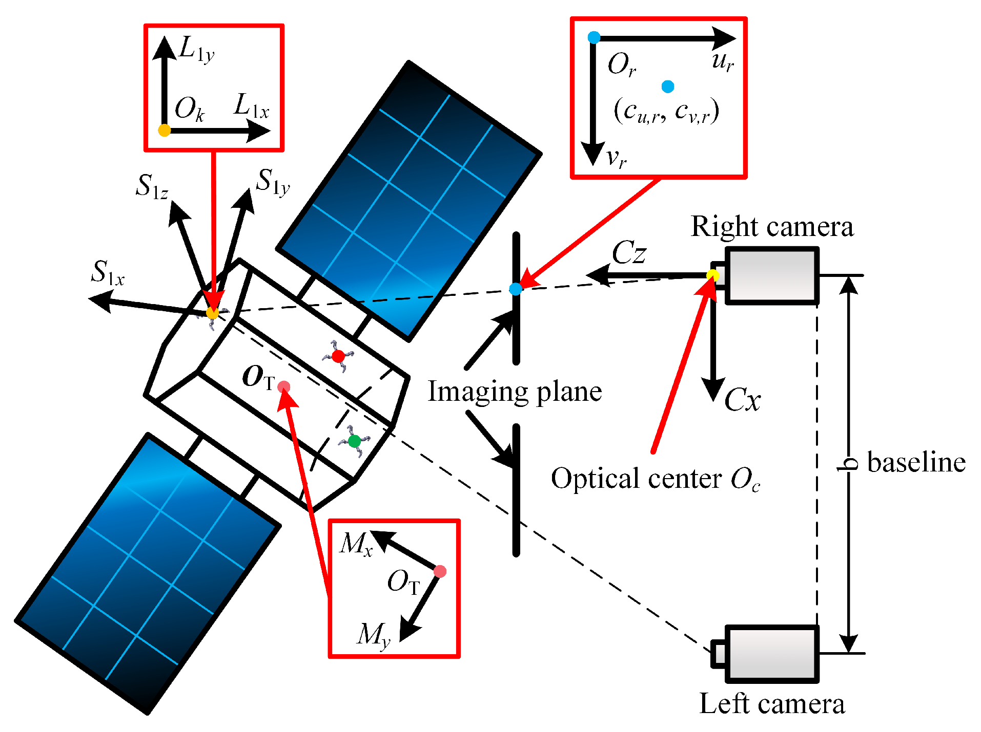
To reduce the processing difficulty of experimental equipment, realize the synchronization of simulations and experiments, we set a large space debris’ simulation model of 2 m × 2 m × 2 m, and attach masses to change the model’s mass distribution (the normalized principal moments of inertia are 2.6, 2, 1). The mass center of the debris is located at (−1, 1, 4) m in frame C. The initial poits are random from (0, 0, 0) m to (−0.9, 0.9, 2.9) m. In simulations and experiments, there are 3 inertial units attached to the space debris, the angle between S k and M is known, and the distances from IMUs to mass center are 1.5 m, 1.6 m, and 1.6 m, respectively. The luminous markers are attached to IMUs’ surface.
Refer to Pesce’s related work [13], we set zero-mean Gaussian to measurement of vision and IMUs. Considering the extreme lighting environment, the visual noise is set as Gaussian distribution with a standard deviation of 2.2 pixels, its value is larger than 1 pixel in reference [13]. Refer to the binocular camera and IMUs used in experiments, the sampling frequency of vision and IMUs are set to 20 Hz and 200 Hz, respectively. Considering the actual measured value and the influence of the space environment, the standard deviation of IMUs’ noise is tripled to factory calibration value. The variance of the angular velocity’s noise is 0.0087 rad/s, the angular acceleration’s noise is 0.01744 rad / s 2 , and the error variance of linear acceleration’s noise is 0.9801 m / s 2 . The initial angular velocity is set to [1, 10, 2] r/min. Iteration is set at per 5 sample points, and the maximum number of iterations is set to 10. The simulation parameters are shown in Table 1 and Table 2.
In order to prove the validity and reliability of the L-M algorithm for the estimation in this paper, we used Monte Carlo analysis to compare the results of the L-M algorithm and the EKF (extended Kalman filter) algorithm on J a , k . One hundred simulations were set, and the results are shown in Table 3.
Shown as Table 3, the L-M algorithm achieved all convergence, while the EKF only converged 87 times. This is due to the fact that the initial value of the 13 non-convergent iterations is far from the true value, and the error of the observation equation is large, which led to the non-convergence of the EKF. While the LM algorithm is less affected by the initial conditions, so full convergence was achieved. In the simulation of convergence, the accuracy of both algorithms could achieve about 0.025. However, the LM algorithm converged faster than EKF due to the good local convergence. Therefore, for the unconstrained optimization in this article, the L-M algorithm with better stability and faster convergence was selected.The simulation results are shown in the figures and tables below.
For the measurement of the moment of inertia, the conversion between the normalized 5-parameter inertia tensor and the normalized 2-parameter principal moment of inertia matrix is obtained by Equation (6). Furthermore, the error of principal moment of inertia is positively related to R M t o S k . To make the figures clearer, this section use the normalized 2-parameter principal moment of inertia to measure the model’s solution effect on the inertia tensor and direction cosine matrix. Two non-uniform normalized principal moments of inertia J a , k , M and J b , k , M are considered. As shown in Figure 4, when the calculating to 2.09 s, the J a , k , M and J b , k , M converged to below 0.03 (dimensionless), which proves that the model has good computational efficiency and a good calculation accuracy. The accuracy meets the subsequent calculation requirements, which will significantly reduce the error of inertial data after denoising. Moreover, because the amount of data required is small, the calculation time is short, which can reduce the impact of random interference.
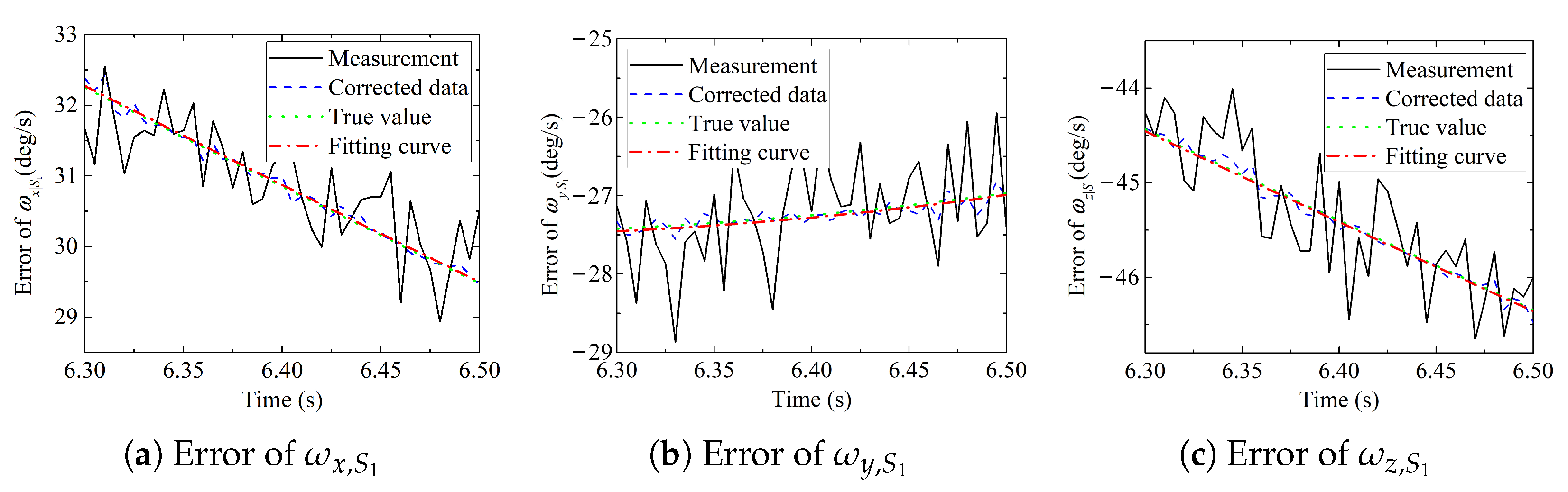
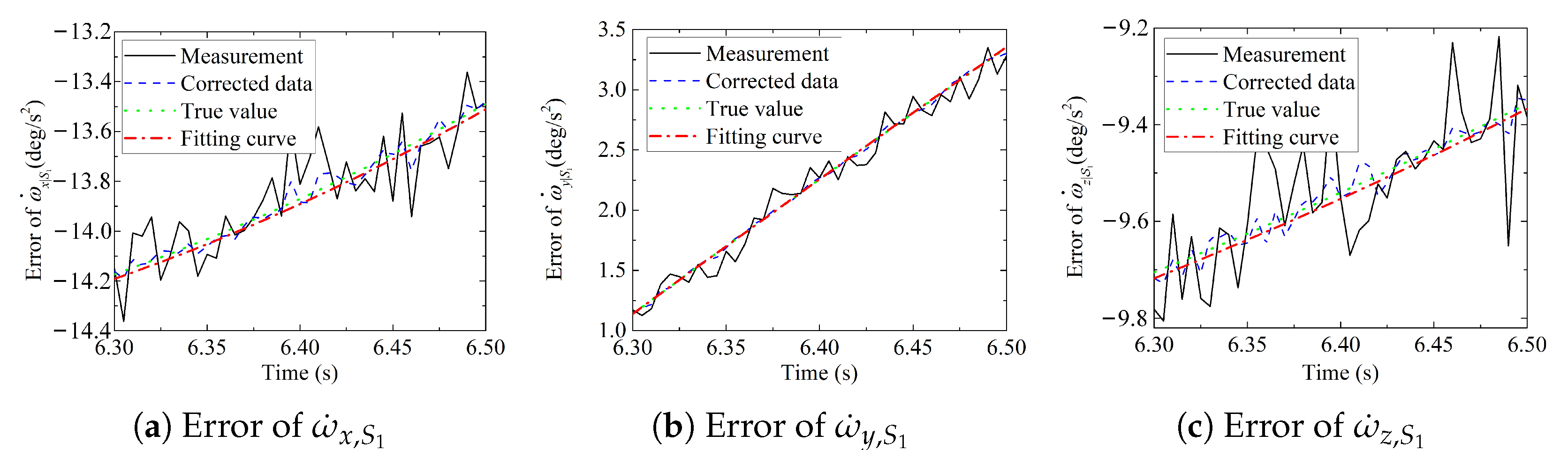
The real-time denoising results are shown in Figure 5, Figure 6 and Figure 7, and Table 4. The triaxial average relative errors of ω were all less than 0.9008%, the triaxial average relative errors of ω ˙ were less than 0.9641%, and the triaxial average relative errors of a were less than 0.9209%, it can be seen that the error was reduced to less than 1% after the denoising of the inertial data, which achieves a better real-time denoising effect and provides good data support for the subsequent calculation.
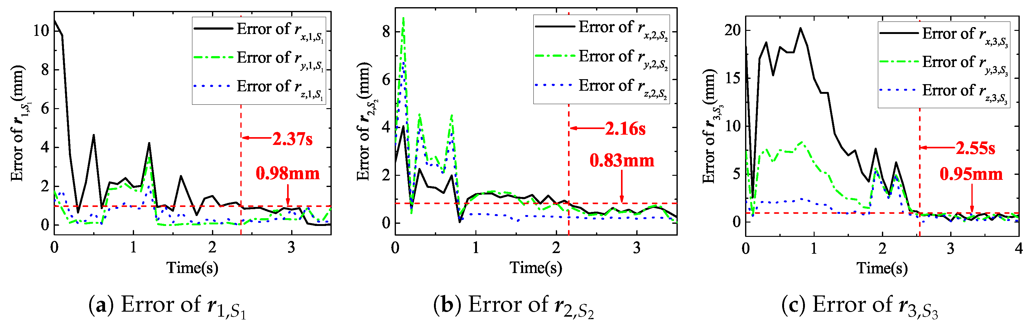
Figure 8 shows the simulation error of the vectors from the mass center O T to the origin of S k . It can be seen that the vectors’ triaxial average error converged below 0.98 mm after 2.55 s. As the process of our algorithm for identifying the mass center is different from existing methods, the comparison for this vector is not given in the paper. However, from the subsequent results of the mass center solution, the accuracy and real-time performance are also in line with the requirements of the de-tumbling and capture operations.
Figure 9 shows the mass-center identification error. When the calculation time reached 6.83 s, the triaxial errors of the mass center converged to less than 0.47 mm. This is an accurate estimation, which can provide a good data benchmark for normalized angular momentum orientation and de-tumbling force positioning.
The Average relative error of R S k t o C ( i ) is shown in Table 5. The m k , l ( k , l = 1, 2, 3) are the elements in R S k t o C ( i ) , and the maximum error was 0.711%, which can provide the good basis for calculating normalized angular momentum.
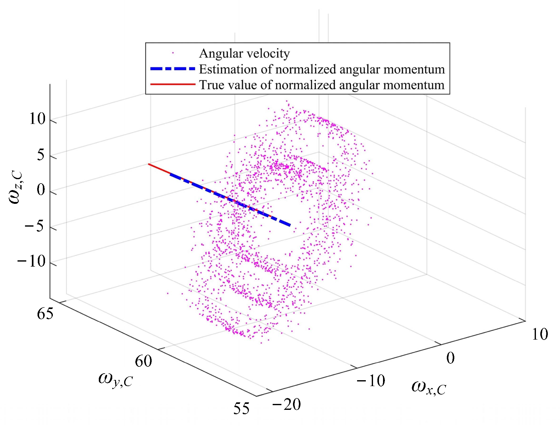
As shown in Figure 10 and Table 6, the normalized angular momentums were estimated, and the relative error of solved L C was less than 0.25%, and the convergence time was less than 7.53 s, which can guide the de-tumbling operation and Improve the efficiency and success rate of de-tumbling.

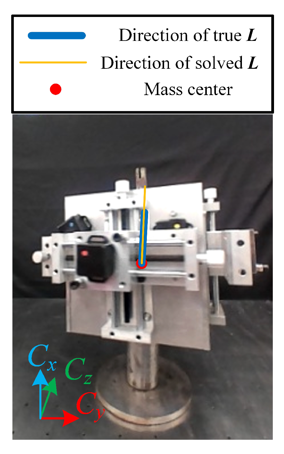
5. Experiments of Dynamic Parameters’ Identification

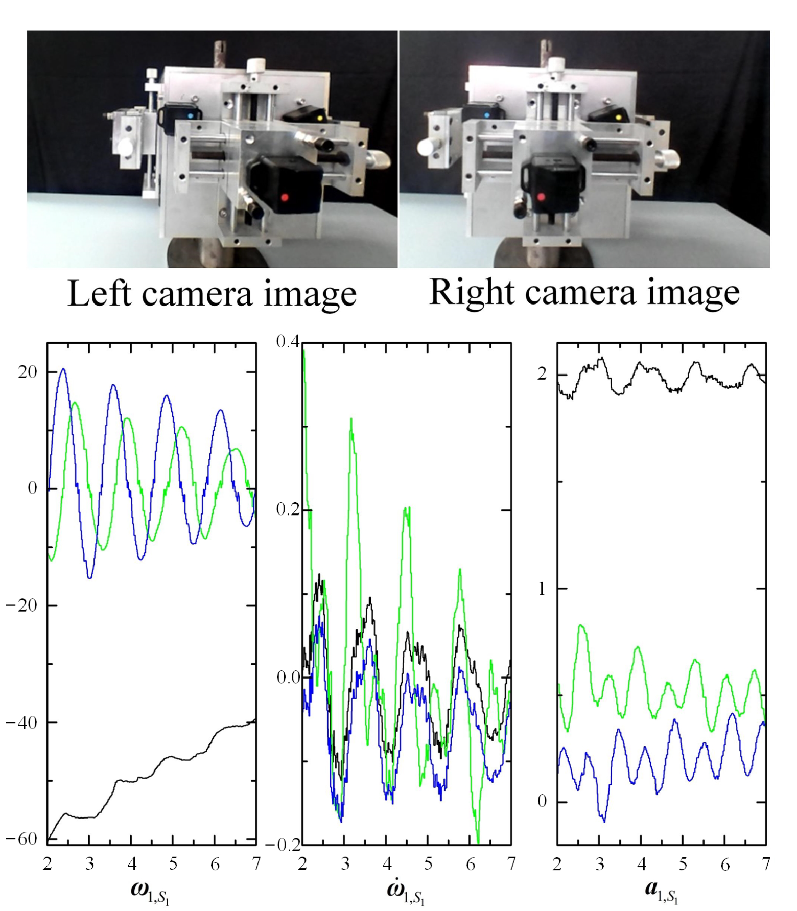
To verify the effectiveness and reliability of our method, experiments in the controlled laboratory scenario are carried out in this section. The designed experiment system is shown in Figure 11, in which the three IMUs are WT-901, with a sampling frequency of 200 Hz and communicate with the host computer through CSMA/CA protocol, and the distance between IMUs and mass center is 0.3 m, 0.32 m, and 0.32 m, respectively. The surface of every IMU is pasted with different color markers to simulate the luminous marker points in the space environment; the binocular vision is MYNTAI-S2110 with a sampling frequency of 20 Hz and a resolution of 720 × 480. The ‘debris’ is a proportionally reduced size model relative to the simulation, with a size of 0.4 m × 0.4 m× 0.4 m, and the center of mass is located at (−0.2 m, 0.2 m, 0.8 m) in frame C. The universal ball is selected as the rotating part to realize the triaxial rotation of the ‘debris’. According to the spacecraft mass adjustment mechanism described in [30], a combined device of slide and metal block is designed as a mechanism for adjusting the mass center. The mass blocks are aluminum alloy block and stainless-steel block which are symmetrically fixed to equipment, and realize different principal moments of inertia in this way, the normalized principal moments of inertia are also 2.6, 2 and 1. The initial angular velocity of experiments is set to correspond to the simulation, and both are [1, 10, 2] r/min. The experimental parameters are shown in Table 7, Table 8 and Table 9.
The experimental data are shown in Figure 12. The periodicity decreasing of angular velocity is caused by gravity torque causing the error of mass adjustment, friction of the universal ball and air resistance. To eliminate the influence of the external moment, the influence of the gravitational moment is fitted by the change of the angle Δ θ ( i ) between the IMU’s axis and the direction of gravity measured by the IMU. The friction and air resistance are, respectively, the constant unknown moment f and s . The distance between the mass center and the rotation center is set to constant unknown quantity l, and the initial angle between the center of mass and the gravity axis is set to θ i n i . The mass m of ‘debris’ is known, and the torque-free Euler equation is changed to the following form:
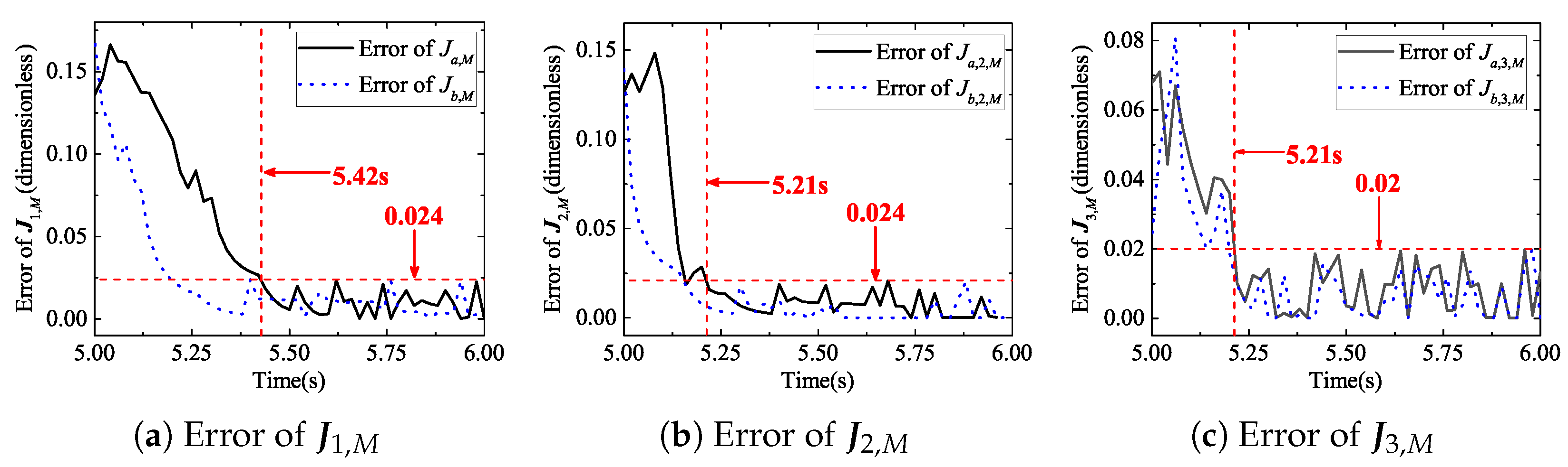
J ω ˙ + ω × J ω = m g l sin θ i n i + Δ θ ( i ) + f + s
The J a , k , M and J b , k , M ’s experimental results are shown as Figure 13. When the calculation reaches 5.42 s, J k , M converges to 0.027 (dimensionless). Compared with the simulation, the convergence time of the algorithm is longer, which is mainly affected by the added solution quantity in Equation (40) and leads to the need for more data points for estimation.
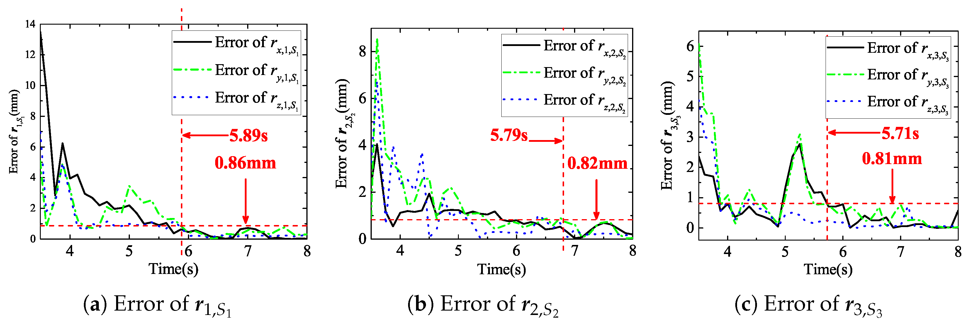
As shown in Figure 14, when the calculation reaches 5.89 s, the triaxial error of the r k , S k decreased to 0.86 mm as reported in Figure 14. Using this error to measure the denoising result, it is known that the average relative error of the measured data of the inertial unit after denoising is less than 1.1%, which proves that this method can achieve a better denoising effect under actual working conditions.
Since the motions of experimental equipment and the Euler–Poinsot motion are the same, they are both fixed-point motion, the identify mass center is replaced by identifying the rotation center. As shown in Figure 15, at 9.21 s, the three-axis error of the mass center location converged below 0.49 mm. Compared with the simulation, the convergence time of the algorithm in the experiment is longer, which is mainly affected by the low resolution of binocular vision.
The experiments’ results of normalized angular moment are shown in Figure 16 and Table 10, Error of L C is less than 0.0081 rad, and the convergence time is less than 10.31 s. Limited by the experimental conditions, the experimental error is slightly larger than the simulation error. However, our method can still provide better guidance for de-tumbling mission.
Table 11 shows the comparison of the simulation and experimental results of our method with the Pesce’s simulation results and the Tweddle’s experimental results (they are all binocular vision method). Because binocular vision is affected by complex spatial lighting conditions, so the convergence time of visial method is more than this method; Tweddle’s method identifies the object as a geometric symmetrical object, so it identifies the geometric center of the fragment feature point as the debris’ mass center, but it has a certain offset when it is used in normal debris, so our recognition error of this method is less than Tweddle’s algorithm. At the same time, this method increases the estimation of the angular momentum’s direction in the de-tumbling frame. The above comparison proves that our method is more in line with the actual needs of de-tumbling and capture mission.

6. Conclusions

In this paper, aiming at identifying dynamic parameters of large space debris such as final stage rockets and failed satellites, a method based on visual and inertial data fusion is proposed, and a binocular camera and IMUs are used to acquire data. The real-time performance of IMU and the positioning advantage of stereo vision is used to improve the identification accuracy of dynamic parameters. Using unconstrained optimization and space debris’ dynamic characteristics, this method reduces the noise of the IMU’s data, and on this basis, the normalized principal moment of inertia, the mass-center location in the ADR coordinate system and the normalized angular momentum of the space debris are better estimated, and a set of active-debris-removal parameters is established. Simulations are carried out with Gaussian white noise. The simulations showed that the normalized principal moment of inertia’s error converges below 0.03 (dimensionless) after 2.09 s. A laboratory experimental system was built. The experiment showed that the normalized principal moment of inertia’s error converged below 0.024 (dimensionless) when the calculation reached 5.42 s. In the simulation, the errors of angular velocity, angular acceleration and linear acceleration were all less than 1%, and the triaxial error of the distance from mass center to IMUs converged below 0.98 mm when the calculation reached 2.55 s. In the experiments, the triaxial errors of the distance from the center of mass to IMU were less than 0.86 mm after 5.89 s, and using this error, we can know the good effect of IMU data’s denoising. For the mass-center location estimations, when the simulation time was more than 6.83 s, the triaxial error of mass-center location converged below 0.47 m, and when the experimental time was more than 9.21 s, the triaxial error of centroid position converged below 0.49 m. In simulations, the transformation matrix from IMUs’ frame to ADR frame was calculated, and the maximum error of the elements in the matrix was 0.711%. The normalized angular moment’s relative error was less than 0.0025 rad after 7.53 s. In the experiments, the normalized angular moment’s relative error was less than 0.0081 rad after 10.31 s, which proves the great calculation effect of the transformation matrix from the IMUs’ frame to ADR frame. The simulations and experiments’ results prove the robustness, high precision and real-time of our method. This method is suitable for space debris de-tumbling and capture missions in LEO, and is also useful for real-time, high accuracy in-orbit missions.
An IMU is used in our method, which is essential to reduce spatial light interference and improve computational efficiency. In addition, the short calculation time proves that the amount of data required by this method is small, which is beneficial to reduce the calculation cost of the on-board computer. To calculate the optimization equation, the L-M algorithm is used. In fact, the L-M algorithm can be further improved to better adapt to this method and increase computational efficiency. In the future, we can use the inertia parameters obtained for 3D reconstruction of space debris, and find the optimal impact location. Moreover, in the next step, using the dynamic parameters estimated in this paper and the impact location, the ADR mission can be carried out.

Author Contributions

Methodology, H.Z.; formal analysis, Y.L.; investigation and writing-original draft preparation, J.Y.; writing—review and editing, J.Y., H.Z., Y.L.; supervision, S.D. All authors have read and agreed to the published version of the manuscript.

Funding

This work was financially supported by the National Natural Science Foundation of China (Number 51575126), the Natural Science Foundation of Hebei Province (Number E2019202132), Hebei Province Higher Education Science and Technology Research Project (Number BJ2019049), Funded by Science and Technology on Space Intelligent Control Laboratory (Number 6142208200101 and 6142208190308), Postgraduate Innovation Funding Project of Hebei Province (Number CXZZSS2020025), Tianjin Key Laboratory of Micro-Low Gravity Environment Simulation Technology Open Subjects (WDZL-2020-01) and Innovation Fund of China Academy of Space Technology (Number CAST-2021-01-11).

Institutional Review Board Statement

Not applicable.

Informed Consent Statement

Not applicable.

Acknowledgments

Thanks to the Hebei University of Technology and Beijing Institute of Spacecraft System Engineering for their financial and equipment support for this project.

Conflicts of Interest

The authors declare no conflict of interest.

References

  1. Sun, C.; Wan, W.; Deng, L. Adaptive space debris capture approach based on origami principle. Int. J. Adv. Robot. Syst. 2019, 16, 1729881419885219. [Google Scholar] [CrossRef] [Green Version]
  2. Endo, Y.; Kojima, H.; Trivailo, P.M. Study on acceptable offsets of ejected nets from debris center for successful capture of debris. Adv. Space Res. 2020, 66, 450–461. [Google Scholar] [CrossRef]
  3. Zhao, P.; Liu, J.; Wu, C. Survey on research and development of on-orbit active debris removal methods. Sci. China Technol. Sci. 2020, 66, 1–23. [Google Scholar] [CrossRef]
  4. Anz-Meador, P.D.; Opiela, J.; Shoots, D.; Liou, J.C. History of On-Orbit Satellite Fragmentations; TM-2018-220037; NASA: Washington, DC, USA, 2018. [Google Scholar]
  5. Celletti, A.; Efthymiopoulos, C.; Gachet, F.; Galeş, C.; Pucacco, G. Dynamical models and the onset of chaos in space debris. Int. J. Non-Linear Mech. 2017, 90, 147–163. [Google Scholar] [CrossRef] [Green Version]
  6. Shan, M.; Guo, J.; Gill, E. Review and comparison of active space debris capturing and removal methods. Prog. Aerosp. Sci. 2016, 80, 18–32. [Google Scholar] [CrossRef]
  7. Tweddle, B.E. Computer Vision-Based Localization and Mapping of an Unknown, Uncooperative and Spinning Target for Spacecraft Proximity Operations; Massachusetts Institute of Technology: Cambridge, MA, USA, 2013. [Google Scholar]
  8. Tweddle, B.E.; Saenz-Otero, A.; Leonard, J.J.; Miller, D.W. Factor Graph Modeling of Rigid-body Dynamics for Localization, Mapping, and Parameter Estimation of a Spinning Object in Space. J. Field Robot. 2015, 32, 897–933. [Google Scholar] [CrossRef]
  9. Flores-Abad, A.; Ma, O.; Pham, K.; Ulrich, S. Factor Graph Modeling of Rigid-body Dynamics for Localization, Mapping, and Parameter Estimation of a Spinning Object in Space. Prog. Aerosp. Sci. 2014, 68, 1–26. [Google Scholar] [CrossRef] [Green Version]
  10. Tweddle, B.E.; Setterfield, T.P.; Saenz-Otero, A.; Miller, D.W. An Open Research Facility for Vision-Based Navigation Onboard the International Space Station. J. Field Robot. 2016, 33, 157–186. [Google Scholar] [CrossRef]
  11. Setterfield, T.P. On-Orbit Inspection of a Rotating Object Using a Moving Observer; Massachusetts Institute of Technology: Cambridge, MA, USA, 2017. [Google Scholar]
  12. Setterfield, T.P.; Miller, D.W.; Saenz-Otero, A.; Frazzoli, E.; Leonard, J.J. Inertial Properties Estimation of a Passive On-orbit Object Using Polhode Analysis. J. Guid. Control. Dyn. 2018, 41, 2214–2231. [Google Scholar] [CrossRef]
  13. Pesce, V.; Lavagna, M.; Bevilacqua, R. Stereovision-based pose and inertia estimation of unknown and uncooperative space objects. Adv. Space Res. 2017, 59, 236–251. [Google Scholar] [CrossRef]
  14. Qiu, S.; Guo, Y.; Xing, J.; Ma, G. Inertia parameter and attitude estimation of space noncooperative tumbling target based on a two-step method. In Proceedings of the IECON 2017-43rd Annual Conference of the IEEE Industrial Electronics Society, Beijing, China, 29 October–1 November 2017; pp. 6555–6560. [Google Scholar]
  15. Bai, X.; Zhou, F.; Xing, M.; Bao, Z. High resolution ISAR imaging of targets with rotating parts. IEEE Trans. Aerosp. Electron. Syst. 2011, 47, 2530–2543. [Google Scholar] [CrossRef]
  16. Opromolla, R.; Fasano, G.; Rufino, G.; Grassi, M. Uncooperative pose estimation with a LIDAR-based system. Acta Astronaut. 2015, 110, 287–297. [Google Scholar] [CrossRef]
  17. Ghio, S.; Martorella, M. Estimation of rotating RSO parameters using radar data and joint time-frequency transforms. In Proceedings of the 7th European Conference on Space Debris, Darmstadt, Germany, 18–21 April 2017; pp. 1–9. [Google Scholar]
  18. Ghio, S.; Martorella, M.; Staglianò, D.; Petri, D.; Lischi, S.; Massini, R. Practical implementation of the spectrogram-inverse Radon transform based algorithm for resident space objects parameter estimation. Sci. Meas. Technol. IET 2019, 13, 1254–1259. [Google Scholar] [CrossRef]
  19. Ghio, S.; Martorella, M.; Staglianò, D.; Petri, D.; Lischi, S.; Massini, R. Experimental Comparison of Radon Domain Approaches for Resident Space Object’s Parameter Estimation. Sensors 2021, 21, 1298. [Google Scholar] [CrossRef] [PubMed]
  20. Meng, Q.; Liang, J.; Ma, O. Identification of all the inertial parameters of a non-cooperative object in orbit. Aerosp. Sci. Technol. 2019, 91, 571–582. [Google Scholar] [CrossRef]
  21. Belokonov, I.V.; Lomaka, I.A. Investigation of the possibility of determining the inertial characteristics and the angular velocity vector of chaotically rotating space debris object using a nanosatellite. In Proceedings of the 2018 25th Saint Petersburg International Conference on Integrated Navigation Systems (ICINS), Saint Petersburg, Russia, 28–30 May 2018; pp. 1–4. [Google Scholar]
  22. Aglietti, G.S.; Taylor, B.; Fellowes, S.; Ainley, S.; Tye, D.; Cox, C.; Zarkesh, A.; Mafficini, A.; Vinkoff, N.; Bashford, K.; et al. RemoveDEBRIS: An in-orbit demonstration of technologies for the removal of space debris. Aeronaut. J. 2020, 124, 1–23. [Google Scholar] [CrossRef]
  23. Forshaw, J.L.; Aglietti, G.S.; Fellowes, S.; Salmon, T.; Retat, I.; Hall, A.; Chabot, T.; Pisseloup, A.; Tye, D.; Bernal, C.; et al. The active space debris removal mission RemoveDebris. Part 1: From concept to launch. Acta Astronaut. 2019, 168, 293–309. [Google Scholar] [CrossRef] [Green Version]
  24. Aglietti, G.S.; Taylor, B.; Fellowes, S.; Salmon, T.; Retat, I.; Hall, A.; Chabot, T.; Pisseloup, A.; Cox, C.; Zarkesh, A.; et al. The active space debris removal mission RemoveDebris. Part 2: In orbit operations. Acta Astronaut. 2019, 168, 310–322. [Google Scholar] [CrossRef] [Green Version]
  25. Underwood, C.; Viquerat, A.; Schenk, M.; Taylor, B.; Massimiani, C.; Duke, R.; Stewart, B.; Fellowes, S.; Bridges, C.; Aglietti, G.; et al. InflateSail De-Orbit Flight Demonstration Results and Follow-On Drag-Sail Applications. In Proceedings of the 69th International Astronautical Congress (IAC), IAC-18-A6.5.2, Bremen, Germany, 1–5 October 2018. [Google Scholar]
  26. Dudziak, R.; Tuttle, S.; Barraclough, S. Harpoon technology development for the active removal of space debris. Adv. Space Res. 2015, 56, 509–527. [Google Scholar] [CrossRef]
  27. Borisov, A.; Mamaev, I.S. Rigid Body Dynamics; Higher Education Press: Beijing, China, 2018; pp. 90–97. [Google Scholar]
  28. Levenberg, K. A method for the solution of certain non-linear problems in least squares. Q. Appl. Math. 1944, 2, 164–168. [Google Scholar] [CrossRef] [Green Version]
  29. Marquardt, D.W. An algorithm for least-squares estimation of nonlinear parameters. J. Soc. Ind. Appl. Math. 1963, 11, 431–441. [Google Scholar] [CrossRef]
  30. Meng, Q.; Liang, J.; Ma, O. Payload and spacecraft technology for GP-B. Adv. Space Res. 2000, 25, 1193–1197. [Google Scholar]
Figure 1. Reference frames and coordinate systems.
Actuators 10 00149 g001
Figure 2. Polhode of space debris.
Actuators 10 00149 g002
Figure 3. Process of mass-center estimation.
Actuators 10 00149 g003
Figure 4. Simulation results: Error of principal moment of inertia.
Actuators 10 00149 g004
Figure 5. Simulation results: Error of angular velocity ( ω S 1 ).
Actuators 10 00149 g005
Figure 6. Simulation results: Error of angular acceleration ( ω ˙ S 1 ).
Actuators 10 00149 g006
Figure 7. Simulation results: Error of angular acceleration ( a 1 , S 1 ).
Actuators 10 00149 g007
Figure 8. Simulation results: Error of r k , S k .
Actuators 10 00149 g008
Figure 9. Simulation results: the error of mass-center location.
Actuators 10 00149 g009
Figure 10. Identification of normalized angular moment.
Actuators 10 00149 g010
Figure 11. Experimental device.
Actuators 10 00149 g011
Figure 12. Experimental data.
Actuators 10 00149 g012
Figure 13. Simulation results: Error of principal moment of inertia.
Actuators 10 00149 g013
Figure 14. Simulation results: Error of r k , S k .
Actuators 10 00149 g014
Figure 15. Experiment results: the error of mass-center location.
Actuators 10 00149 g015
Figure 16. Identification of normalized angular moment.
Actuators 10 00149 g016
Table 1. Simulation parameters of large space debris model.
Size of
Model (m)
J M
(Dimensionless)
O T (m)Distance
from IMU to
O T (m)
The Maximum
Number of
Iterations
Initial Poits
of Iterations (m)
Initial
ω (r/min)
2 × 2 × 21, 2, 2.6
(use attached
mass block)
(−1, 1, 4)1.5, 1.6, 1.6
(three IMUs)
10
(per 5 points)
Random from
(0, 0, 0) to
(−0.9, 0.9, 2.9)
[1, 10, 2]
Table 2. Simulation parameters of sensors.
Angular
Velocity
Noise (rad/s)
Angular
Acceleration
Noise (rad/ s 2 )
Linear
Acceleration
Noise (m/ s 2 )
Visual Noise
(Pixel)
Sampling Frequency
of IMU (Hz)
Sampling Frequency
of Vision (Hz)
0.00870.017440.9801220020
Table 3. Comparison of L-M algorithm and EKF algorithm.
AlgorithmNumber of SimulationsNumber of ConvergencesMean ErrorTime (s)
L-M1001000.0292.09
EKF100870.0254.01
Table 4. Simulations results: error of redundant IMUs data’ denoising.
Type of DataAxisAverage Relative Error (%)
x0.9008
Angular velocityy0.7631
z0.6487
x0.9641
Angular accelerationy0.6619
z0.4576
x0.8216
Angular velocityy0.7254
z0.9209
Table 5. Simulation results: average relative error of R S k t o C ( i ) .
m 11 m 12 m 13 m 21 m 22 m 23 m 31 m 32 m 33
Average relative error (%)0.5610.7110.6890.6600.6940.6050.6820.6230.674
Table 6. Simulation results: average relative error of R S k t o C ( i ) .
AxisDirection of Solved L C (rad)Direction of True L C (rad)Convergence Time (s)
x1.72921.72677.26
y0.15840.15596.95
z1.57051.57097.53
Table 7. Parameters of experimental equipment.
Size of
Model
(m)
J M
(Dimensionless)
O T (m)Distance from
IMU to
Mass Center (m)
Initial Poits of
Iterations (m)
The Maximum
Number of
Iterations
0.4 × 0.4 × 0.41, 2, 2.6
(use attached
mass block)
(−0.2, 0.2, 0.8)0.3, 0.32, 0.32
(three IMUs)
Random from
(0, 0, 0) to
(−0.9, 0.9, 2.9)
10
(per 5 points)
Table 8. Parameters of Binocular vision.
Binocular CameraResolution of CameraInitial Angular Velocity (r/min)Sampling Frequency
(Hz)
MYNTAI-S2110720 × 480[1, 10, 2]20
Table 9. Parameters of IMUs.
IMUsSampling Frequency (Hz)Error of Gyroscope on
Nameplate Marking (rad/s)
Error of Accelerometer
on Nameplate Marking (m/s 2 )
WT-9012000.000870.09801
Table 10. Experiment results: average relative error of R S k t o C ( i ) .
AxisDirection of Solved L C (rad)Direction of True L C (rad)Convergence Time (s)
x0.57580.57119.53
y1.26921.26119.77
z1.43101.435810.31
Table 11. Comparison of the algorithm in this paper with existing binocular vision methods.
TypeError of J M Error of Sensors’ Data (%)Error of O T , C (mm)Error of L C (rad)Time
Simulations0.031.00.470.00257.53
Experiments0.0241.10.490.008110.31
Pesce [13]0.0436.9--34.6
Tweddle [7]0.02086.14.34-15.6
Publisher’s Note: MDPI stays neutral with regard to jurisdictional claims in published maps and institutional affiliations.

