Active Disturbance Rejection Control for Position Tracking of Electro-Hydraulic Servo Systems under Modeling Uncertainty and External Load

Abstract

In this paper, an active disturbance rejection control is designed to improve the position tracking performance of an electro-hydraulic actuation system in the presence of parametric uncertainties, non-parametric uncertainties, and external disturbances as well. The disturbance observers (Dos) are proposed to estimate not only the matched lumped uncertainties but also mismatched disturbance. Without the velocity measurement, the unmeasurable angular velocity is robustly calculated based on the high-order Levant’s exact differentiator. These disturbances and angular velocity are integrated into the control design system based on the backstepping framework which guarantees high-accuracy tracking performance. The system stability analysis is analyzed by using the Lyapunov theory. Simulations based on an electro-hydraulic rotary actuator are conducted to verify the effectiveness of the proposed control method.

1. Introduction

Electro-hydraulic servo systems (EHSSs) have been widely employed for years in a wide range of industrial applications such as load simulators [1], robot manipulators [2,3,4,5,6], vehicle active suspension [7,8], and hydraulic press [9] due to their advantages of high produced force/torque, high stiffness, high power-to-weight ratio, high load efficiency, and fast and smooth response [10]. However, high-accuracy position tracking control of electro-hydraulic systems is still challenging owing to highly nonlinear characteristics [11], parametric uncertainties (i.e., significant changes in effective bulk modulus and viscosity with temperature, etc.), unmodeled uncertainties, and external disturbances.

To deal with the nonlinearities of the electro-hydraulic systems, feedback linearization methods such as full-state feedback linearization [12], input-output feedback linearization [13], and partial input feedback linearization [14] were investigated under the assumption that the exact model information is available. In [15], a modified feedback linearization-based position control with supply pressure uncertainty was introduced to improve the tracking performance; however, the parametric uncertainties have not been fully considered in this work. In addition, the feedback linearization controller [16] was proven to not be robust in modeling uncertainty and sensor noise due to the high-order derivative terms in control inputs. Hence, to overcome the challenge of modeling uncertainty, nonlinear robust control, such as sliding mode control (SMC), is proposed in several studies [17,18,19]. The main advantage of SMC that it is well established, simple, and widely applicable [20] to hydraulic servo systems. It has proven to be robust in modeling inaccuracies satisfied matching conditions. If the chosen switching gains of SMC are bigger than the upper bound on the uncertainties, robust stabilization can be achieved [21]. However, in practice, the upper bound is partly known or even completely unknown, so the switching gains must be sufficiently large to suppress the influence of the uncertainties. The adoption of high-gain feedback control and the sign function in the control law cause chattering problems [22], resulting in insufficient control accuracy, high heat losses in electrical power circuits, and high wear of moving mechanical parts [23]. Therefore, some modifications of the SMC approach [24,25,26,27] were introduced to reduce these chattering effects, but there is a tradeoff between tracking accuracy and chattering. Overall, the parametric uncertainties have not been effectively treated in these works. To cope with the parametric uncertainties, the methodology of adaptive control, which utilizes the adaptive mechanism to update the system parameters in the control design, has been studied for the past decades [28,29]. Based on this adaption technique, the gains of the controller can be significantly reduced. By merging adaptive control and robust control, nonlinear adaptive robust control (ARC) approaches [30,31] have been introduced to obtain better performance. In these studies, only bounded tracking performance can be achieved in the presence of mismatched and/or matched disturbances. To obtain an asymptotic tracking performance, a robust integral of the sign of the error (RISE)-based adaptive control [29] has been investigated where unknown parameters are estimated via adaptive technique and all unmodeled uncertainties are compensated by the RISE feedback. However, in this study, the disturbances are assumed to be bounded up to the second-order derivative, therefore this assumption might be restricted in some real applications. Generally, in the above-mentioned works, although model uncertainties have been carefully considered, the influence of external disturbances, i.e., torque/force while interacting with the environment, have not been fully addressed. Therefore, to enhance the tracking performance these disturbances are needed to be estimated and compensated in the control system design.

To deal with the effects of the external disturbances on the control system, disturbance observers (DOs) have been investigated for years with the assumption that their derivatives are bounded [32]. Typically, disturbance observers are broadened to estimate not only the external disturbances but also the model uncertainties. Disturbance and uncertainty are lumped in a generalized term, which is called lumped uncertainties/disturbances. Active disturbance rejection control (ADRC) approaches have been introduced in recent years with various structures to improve the system performance in the presence of disturbances and unmodeled uncertainties such as high-gain disturbance observer [33,34], sliding perturbation observer [35], uncertainty and disturbance estimator (UDE) [36,37], sliding mode observer (SMO) for state and disturbance estimation [38], extended disturbance observer [9], adaptive high gain observer [39], and high-order disturbance observer (DOB) [40]. Among them, extended state observers (ESOs) have been widely used in many works [10,11,19,41,42,43,44] in recent years because they can estimate not only the unmeasurable system states but also the external disturbances. For example, in [19], an extended state observer (ESO)-based control for a hydraulic rotary actuator originated from [45] was proposed to approximate angular velocity and matched disturbance by using an extended state. In this paper, the mismatched disturbance was only attenuated by using a high-gain ESO. The modification of ESO [19] was introduced in [10] by separating the original system into two subsystems to obtain better performance in which the matched and mismatched disturbances are simultaneously estimated. An integral sliding mode backstepping controller based on ESO for the asymmetric electro-hydrostatic actuator was introduced in [44]. However, from the design of the ESO, one can observe that the disturbance estimation performance depends on not only the physical disturbance in the real system but also the unmeasurable state estimation which currently is estimated by the ESO. In contrast, the state estimation of ESO is essentially based on Luenberger observer, which can be improved by exact differentiators [46,47]. Hence, combining DOs and exact differentiators is potential to produce a better disturbance estimation compared to the ESO.

Inspired by the aforementioned discussion, this paper proposes a novel active disturbance rejection control to improve the tracking performance of a hydraulic servo system. In this paper, a highly accurate and robust Levant’s differentiator [48] is applied to exactly calculate the angular velocity of the actuator. Based on that, two disturbance observers (DOs) with the linear structure are proposed to estimate the matched and mismatched disturbances in the subsystems then the estimated disturbances are fed back into the control law. The DOs-based backstepping controller is proposed to attenuate the influence of the disturbances, unmodeled uncertainties caused by weak modeling, and parameter perturbations as well. The stability of the closed-loop system is proven using Lyapunov theory. Simulations are conducted in comparison with other control approaches to show the superiorities of the proposed control algorithm.

This paper is organized as follows: Section 2 presents the studied hydraulic system model. The entire control system design including state observer, disturbance observers, and backstepping control, and the system stability analysis are introduced in Section 3. Section 4 contains the simulation results. The conclusion is provided in Section 5.

2. System Modeling

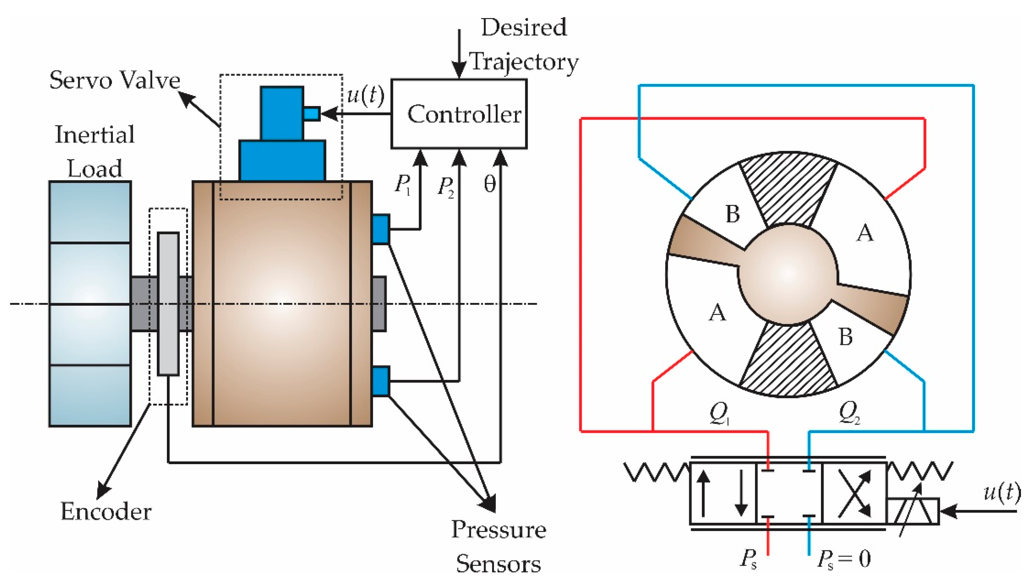
The valve-controlled electro-hydraulic system is illustrated in Figure 1. The hardware configuration of the system is thoroughly depicted on the left-hand side of this figure. In this system, the pressures of two chambers of the hydraulic actuator and the position of the inertial load are measured by two pressure sensors and an encoder, respectively. The information from these sensors is fed back to the controller to generate the control action. The hydraulic circuit of the system is presented on the right-hand side of Figure 1.

To examine the system transparently, the total system can be divided into three subsystems including the mechanical system, servo valve, and hydraulic system. In the mechanical system, we study the motion dynamics of the actuator under the torque of the actuator. Then, the model of the servo valve is thoroughly inspected. Finally, the hydraulic system is also examined in detail. In both cases, the parametric uncertainties, unmodeled uncertainties, and disturbances are carefully investigated.

2.1. Mechanical System Modeling

The motion dynamics of the inertial load is presented as follows

$$J\ddot{\theta }=T_h-F_f\left(\dot{\theta }\right)-F_d\left(\theta ,\dot{\theta },t\right)$$

(1)

where $T_h$ is the torque generated by the hydraulic pressure difference between two chambers A and B of the actuator; $J$ and $\theta$ are the moment of inertia and the angular displacement of the load, respectively; $F_f(\dot{\theta })=B\dot{\theta }$ is the modeled smooth friction dynamics with $B$ is the coefficient of the viscous friction; $F_d(\theta ,\dot{\theta },t)$ represents the disturbances, parameter variations, and unmodeled uncertainties.

The hydraulic torque of the actuator is computed as

$$T_h=P_L{D}_m$$

(2)

where the load pressure $P_L=P_1-P_2$ is the pressure difference between two chambers of the actuator; $P_1$ and $P_2$ are the pressures at the chamber A and chamber B, respectively; $D_m$ represents the radian displacement of the actuator.

Substituting (2) into (1), one obtains

$$J\ddot{\theta }=P_L{D}_m-F_f\left(\dot{\theta }\right)-F_d\left(\theta ,\dot{\theta },t\right)$$

(3)

2.2. Servo-Valve Modeling

The dynamic behavior of a servo-valve includes many parameters. Thereby, some of the parameters may only be known within some ranges, or even completely unknown. However, based on the information about its step responses and/or frequency responses, the servo-valve dynamics was approximated in a simple model for various control objectives. In [49], the servo-valve dynamics model was estimated by a second-order transfer function without loss of accuracy as follows:

$${\ddot{x}}_v+2{\zeta }_v{\omega }_v{\dot{x}}_v+{\omega }_v^2{x}_v+f_v\mathrm{sign}\left({\dot{x}}_v\right)={\omega }_v^2{k}_{v}u$$

(4)

where ${\omega }_v$ is the natural frequency; ${\zeta }_v$ is the damping coefficient; $k_v$ represents the valve coefficient; $x_v$ is the valve spool displacement; $f_v$ takes into account the valve hysteresis and response sensitivity; $u$ is the control input voltage applied to the valve, and $\mathrm{sign}(·)$ is the standard signum function.

In a wide range of valve-controlled hydraulic applications, the valve dynamics are always much more rapid than the dynamics of other components in the system. Moreover, the hysteresis of the servo-valve is also neglected [3]. Therefore, the dynamics of the servo valve can be ignored without performance degradation in the control systems. For the sake of simplicity, the reduced model of the servo-valve can be presented as follows [19]:

$$x_v=k_{v}u$$

(5)

where $k_v$ is the gain of the control voltage $u$ and it can be calculated by using the specification of the servo valve.

2.3. Hydraulic Actuator Modeling

Based on the definition of the effective bulk modulus, the load pressure dynamics can be defined as [19]

$$\frac{V_t}{4{\beta }_e}{\dot{P}}_L=-D_m\dot{\theta }-C_t{P}_L+Q_L+q\left(t\right)$$

(6)

where $V_t$ is the total control volume of the hydraulic motor; ${\beta }_e$ is the effective bulk modulus of the hydraulic oil; $C_t$ is the total coefficient of the overall internal leakage due to the pressure difference between chambers of the actuator; $q(t)$ is the lumped uncertainties caused by complicated internal leakage, unmodelled pressure dynamics, and parameter deviations; $Q_L$ is the load flow.

The load flow $Q_L$ is defined as

$$Q_L=\frac{1}{2}\left(Q_1+Q_2\right)$$

(7)

with $Q_1$ is the supplied flowrate to chamber A, i.e., forward chamber, and $Q_2$ is the returned flowrate from chamber B, i.e., reverse chamber. Moreover, the load flow can be computed as follows:

$$Q_L=C_{d}w{x}_v\sqrt{\frac{1}{\rho }\left(P_s-\mathrm{sign}\left(x_v\right)P_L\right)}$$

(8)

where $C_d$ is the discharge coefficient; $w$ represents the spool valve area gradient; $\rho$ is the density of the oil; and $P_s$ is the supply pressure.

Substituting (5) into (8), the load flow can be transformed into

$$Q_L=k_{t}u\sqrt{\left(P_s-\mathrm{sign}\left(u\right)P_L\right)}$$

(9)

where $k_t=C_d{k}_{v}w\sqrt{1/\rho }$ is the total flow gain with respect to control voltage $u$.

2.4. System Modeling

The total system model is constructed by the mechanical system model (3), the hydraulic system model described by (6) and (9) which already consist of the servo-valve model (5).

Define the state variables as ${\left[x_1,x_2,x_3\right]}^T={\left[\theta ,\dot{\theta },D_m{P}_L/J\right]}^T$. Based on that, the state-space representation of the studied system can be expressed as

$$\{\begin{array}{l}{\dot{x}}_1=x_2\hfill \\ {\dot{x}}_2=x_3+{\phi }_1\left(x_2\right)+d_1\left(x,t\right)\hfill \\ {\dot{x}}_3={\phi }_2\left(x_2,x_3\right)+g\left(x_3,u\right)u+d_2\left(x,t\right)\hfill \end{array}$$

(10)

where

$$\begin{array}{l}{\phi }_1\left(x_2\right)=-\frac{B}{J}{x}_2\\ d_1\left(x,t\right)=-\frac{F_d\left(x_1,x_2,t\right)}{J}\\ {\phi }_2\left(x_2,x_3\right)=-\frac{4D_m^2{\beta }_e}{J{V}_t}{x}_2-\frac{4{\beta }_e}{V_t}{C}_t{x}_3\\ g\left(x_3,u\right)=\frac{4D_m{\beta }_e{k}_t}{J{V}_t}\sqrt{P_s-\frac{J}{D_m}{x}_3\mathrm{sign}\left(u\right)}\\ d_2\left(x,t\right)=\frac{4D_m{\beta }_e}{J{V}_t}q\left(t\right)\end{array}$$

(11)

In the system model, two terms, $d_1(x,t)$, which is the acceleration disturbance, and $d_2(x,t)$, which is the jerk disturbance, are the mismatched and matched lumped disturbances that take into account parametric uncertainties, unmodeled uncertainties, and external disturbances. These terms will be estimated and then fed back to the controller to compensate for their effects. The approximations of these terms are considered in the process of the controller design phase thoroughly in the following section.

3. Controller Design

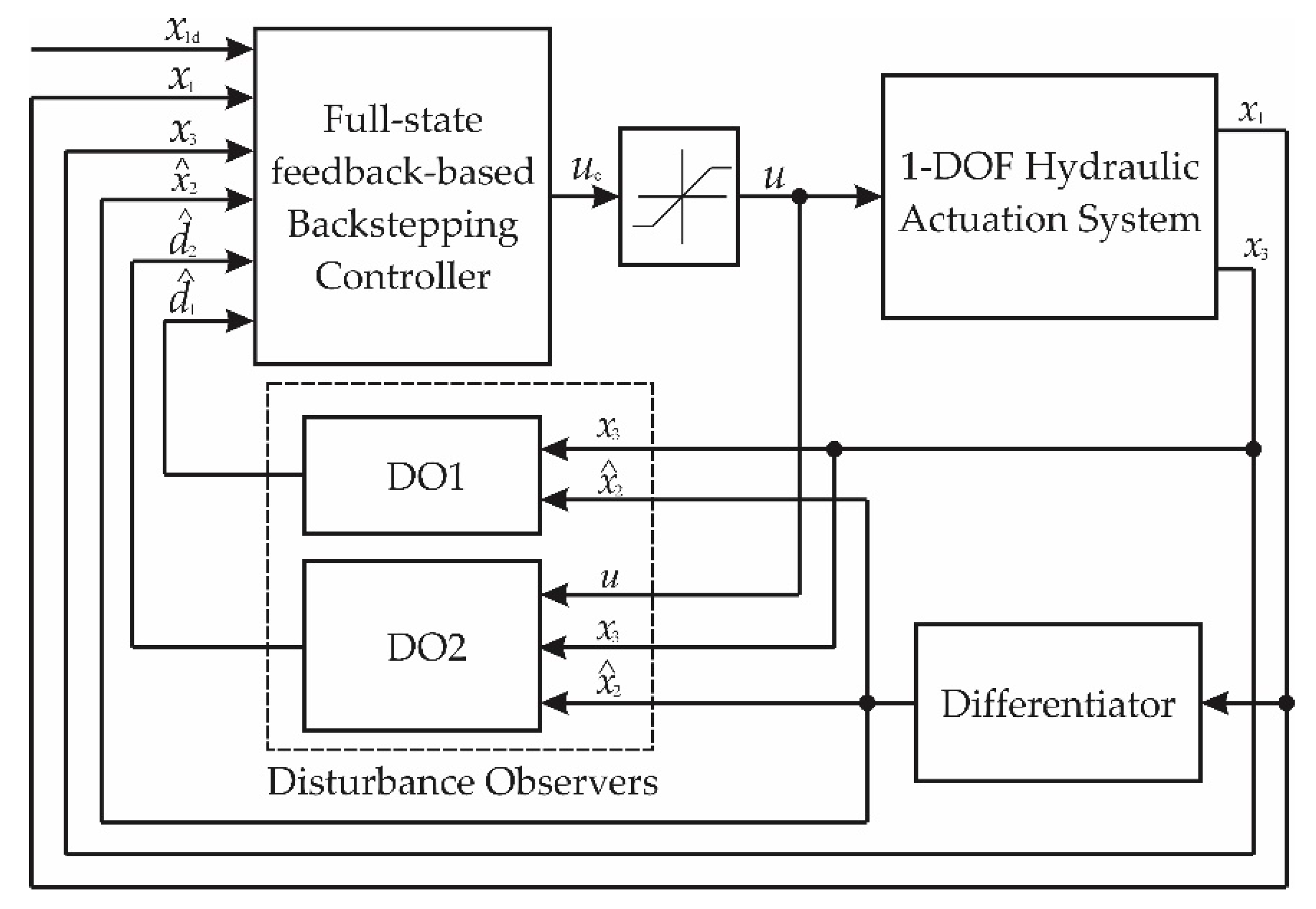
The proposed control scheme is designed to improve the tracking performance and robustness with respect to the uncertainties of the hydraulic system. In this stage, nominal system parameters are used to design the observers and the controller. The modeling errors are lumped to the unmodeled terms $d_1$ and $d_2$ in the second and third equations of (10). The proposed control system is demonstrated in Figure 2.

In this control system, the state observer based on the Levant’s differentiator is designed to accurately approximate the angular velocity of the inertial load. The output of this observer is fed back to the controller and two disturbance observers as well. The disturbance observers are constructed to estimate the lumped uncertainties $d_1$ and $d_2$, then they are integrated in the control design step to compensate for their effects on the closed-loop control system. The controller is synthesized by using the backstepping method, which utilizes the measured states (the angular position and the pressures of chambers of the actuator), estimated state (angular velocity) produced by state observer, and the estimation of unmodeled uncertainties are generated by the disturbance observers. This control algorithm guarantees globally bounded tracking performance in the presence of the modeling error and unmodeled uncertainties.

Before the observer and controller design stage, some assumptions are given as the following:

Assumption 1.

The lumped disturbances are bounded and smooth enough, and their first-order derivatives are bounded by known constants.

$$\begin{array}{l}\left|d_1\right|\le d_1^{\ast };\left|{\dot{d}}_1\right|\le {\dot{d}}_1^{\ast }\\ \left|d_2\right|\le d_2^{\ast };\left|{\dot{d}}_2\right|\le {\dot{d}}_2^{\ast }\end{array}$$

(12)

Assumption 2.

The pressures$P_1$and$P_2$are both bounded by the supply pressure$P_s$. The absolute value of the load pressure is sufficiently smaller than$P_s$to guarantee the function$g(x_3,u)$is far away from zero.

Assumption 3.

The function${\phi }_1(x_2)$is globally Lipschitz with respect to$x_2$;${\phi }_2(x_2,x_3)$is also globally Lipschitz with respect to$x_2$. There exist known constants$c_1,c_2$such that:

$$\{\begin{array}{l}\left|{\phi }_1\left(x_2\right)-{\phi }_1\left({\widehat{x}}_2\right)\right|\le c_1{\tilde{x}}_2\\ \left|{\phi }_2\left(x_2,x_3\right)-{\phi }_2\left({\widehat{x}}_2,x_3\right)\right|\le c_2{\tilde{x}}_2\end{array}$$

(13)

Assumption 4.

The desired position trajectory${\theta }_d\left(t\right)=x_{1d}\left(t\right)$, its first-order and second-order derivatives are bounded.

Lemma 1.

Consider the inequality

$$\dot{x}\left(t\right)\le -\sigma x\left(t\right)+\upsilon$$

(14)

with $\sigma$ and $\upsilon$ are known positive constants.

The solution of equality defined by (14) satisfies the following inequality

$$\underset{t\to \infty }{\lim }\left(x\left(t\right)\right)\le \frac{\upsilon }{\sigma }$$

(15)

Proof of Lemma 1:

See Appendix A. □

3.1. State Observer Design

The state observer is designed to estimate the angular velocity of the inertial load based on the information from the position sensor. In this paper, a second-order Levant’s differentiator [46] is employed to estimate exactly and in a finite time the first-order derivative of the position of the inertial load $x_1\left(t\right)$.

The second-order Levant’s differentiator is mathematically formulated as follows

$$\{\begin{array}{l}{\dot{y}}_1=v_1;v_1=-{\lambda }_1{\left|y_1-x_1\right|}^{2/3}sign\left(y_1-x_1\right)+y_2\\ {\dot{y}}_2=v_2;v_2=-{\lambda }_2{\left|y_2-v_1\right|}^{1/2}sign\left(y_2-v_1\right)+y_3\\ {\dot{y}}_3=-{\lambda }_{3}sign\left(y_3-v_2\right)\end{array}$$

(16)

where ${\lambda }_1,{\lambda }_2,{\lambda }_2$ are the parameters of the differentiator that are positive constants. The trade-off is as follows: the larger the parameters, the faster the convergence and the higher sensitivity to input noises and the sampling step. The estimated angular velocity is defined as

$${\widehat{x}}_2=y_2$$

(17)

The stability of this differentiator has been proven in previous works [48]. In the steady-state condition, the estimation error ${\tilde{x}}_2=x_2-{\widehat{x}}_2$ of the angular velocity and its derivative satisfy the following equations:

$$\begin{array}{l}\left|{\tilde{x}}_2\right|\le \alpha \\ \left|{\dot{\tilde{x}}}_2\right|\le \beta \end{array}$$

(18)

where $\alpha$ is the arbitrary small positive constant depending on the selection of differentiator parameters and $\beta$ is a bounded constant that is defined as

$$\beta =\frac{\left|{\tilde{x}}_{2\max }-{\tilde{x}}_{2\min }\right|}{T}=\frac{2\alpha }{T}$$

(19)

with $T$ being the sampling time.

3.2. Disturbance Observer Design

The disturbance observers are designed to estimate the lumped uncertainties of the mechanical and hydraulic systems. Then, the estimated values are fed back to the control law to compensate for their effects on the control system.

Consider the subsystem that is represented in the second equation of (10) as

$${\dot{x}}_2=x_3+{\phi }_1\left(x_2\right)+d_1$$

(20)

The first disturbance observer is constructed to approximate the mismatched lumped uncertainties in the mechanical system, which is depicted as

$$\{\begin{array}{l}{\widehat{d}}_1=z_1+l_1{\widehat{x}}_2\hfill \\ {\dot{z}}_1=-l_1{\widehat{d}}_1-l_1\left(x_3+{\phi }_1\left({\widehat{x}}_2\right)\right)\hfill \end{array}$$

(21)

where $z_1$ is an intermediary variable of the observer, $l_1$ is the observer gain with $l_1>0$.

Define the estimation error as $e_{d1}=d_1-{\widehat{d}}_1$. The estimation error dynamics is calculated as

$${\dot{e}}_{d1}=-l_1{e}_{d1}-l_1{\tilde{\phi }}_1+l_1{\dot{\tilde{x}}}_2+{\dot{d}}_1$$

(22)

where

$${\tilde{\phi }}_1={\phi }_1\left(x_2\right)-{\phi }_1\left({\widehat{x}}_2\right)$$

(23)

Theorem 1.

Based on Assumptions 1 and 3, the disturbance observer (21) which utilizes the state estimation (17) guarantees that the disturbance estimation error in (22) can be bounded in an arbitrarily small region based on the selection of the DO gain.

Proof of Theorem 1:

See Appendix B. □

Similarly, we consider the second subsystem to be defined as

$${\dot{x}}_3={\phi }_2\left(x_2,x_3\right)+g\left(x_3,u\right)u+d_2\left(x,t\right)$$

(24)

The second disturbance observer is designed to estimate the lumped uncertainties of the subsystem defined as follows

$$\{\begin{array}{l}{\widehat{d}}_2=z_2+l_2{x}_3\hfill \\ {\dot{z}}_2=-l_2{\widehat{d}}_2-l_2\left[g\left(u,x_3\right)u+{\phi }_2\left({\widehat{x}}_2,x_3\right)\right]\hfill \end{array}$$

(25)

where $l_2$ is the disturbance observer gain with $l_2$ is selected such that $l_2>0$.

Define the estimation error $e_{d2}=d_2-{\widehat{d}}_2$. The estimation error dynamics is computed as

$${\dot{e}}_{d2}=-l_2{e}_{d2}-l_2{\tilde{\phi }}_2+{\dot{d}}_2$$

(26)

where

$${\tilde{\phi }}_2={\phi }_2\left(x_2,x_3\right)-{\phi }_1\left({\widehat{x}}_2,x_3\right)$$

(27)

Theorem 2.

The disturbance observer (25) based on Assumptions 1 and 3, which utilizes the state estimation (17), guarantees that the disturbance estimation error in (26) can be bounded in an arbitrarily small region based on the selection of the DO gain.

Proof of Theorem 2:

See Appendix C. □

Remark 1.

The proposed DOBs are able to compensate for not only the external disturbances but also model uncertainties caused by large parameter variations and weak modeling as long as Assumption 1 is satisfied.

3.3. Backstepping Controller Design

The proposed controller is synthesized by using the recursive backstepping method based on the measured states, estimated state, and approximated lumped uncertainties. The design procedure is intuitive because the unmatched uncertainty in the second equation and the matched uncertainty in the third equation of (10) have been completely estimated in the previous sections.

The state errors $e_i\left(i=1,2,3\right)$ are defined as

$$\{\begin{array}{l}{e}_1=x_1-x_{1d}\\ e_2=x_2-x_{2d}\\ e_3=x_3-x_{3d}\end{array}$$

(28)

where $x_{1d}$ is the desired position trajectory, $x_{2d}$ and $x_{3d}$ are the virtual control inputs. Based on the estimated state and observed disturbances, the virtual control inputs are designed to stabilize the subsystems as follows:

$$\{\begin{array}{l}{x}_{2d}=-k_1{e}_1+{\dot{x}}_{1d}\\ x_{3d}=-{\phi }_1\left({\widehat{x}}_2\right)-k_1\left({\widehat{x}}_2-{\dot{x}}_{1d}\right)+{\ddot{x}}_{1d}-k_2\left({\widehat{x}}_2-x_{2d}\right)-{\widehat{d}}_1\end{array}$$

(29)

where $k_1$ and $k_2$ are positive feedback gains. The virtual control function $x_{3d}$ is designed for the virtual control input $x_3$, such that the output tracking performance is ensured.

The actual control input $u$ is designed to stabilize the whole system, which is defined as

$$u=\frac{1}{g\left(x_3,u\right)}\left(-{\phi }_2\left({\widehat{x}}_2,x_3\right)-{\dot{x}}_{3d}-k_3\left(x_3-x_{3d}\right)-{\widehat{d}}_2\right)$$

(30)

The state error dynamics of the augmented system is given by

$$\{\begin{array}{l}{\dot{e}}_1=-k_1{e}_1+e_2\hfill \\ {\dot{e}}_2=-k_2{e}_2+e_3+{\tilde{\phi }}_1+\left(k_1+k_2\right){\tilde{x}}_2+e_{d1}\hfill \\ {\dot{e}}_3=-k_3{e}_3+{\tilde{\phi }}_2+e_{d2}\hfill \end{array}$$

(31)

Theorem 3.

Based on Assumption 1, 2, and 3, the control laws in (29) and (30), which employs the estimated state in (17) and the estimation values of disturbances in (21) and (25) guarantee the ultimately uniformly bounded tracking performance of the system (10) under the presence of uncertain nonlinearities and external disturbances.

Proof of Theorem 3:

See Appendix D. □

4. Simulation Results

4.1. Simulation Setup

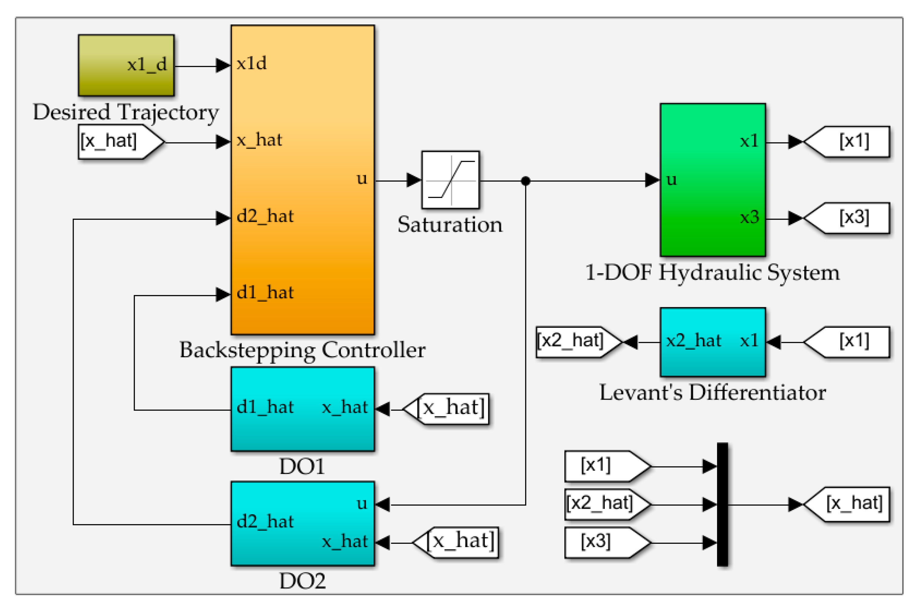
In this section, numerical simulations are conducted to verify the superior effectiveness of the proposed algorithm. The simulations were performed on MATLAB/Simulink 2019b, using Runge-Kuta solver with a fixed step size T = 10⁻³s as shown in Figure 3.

The system parameters of the hydraulic system [19] are listed in the following

Table 1. The hydraulic system parameters.

Parameter	Value	Parameter	Value
$J$($\mathrm{kg}\cdot {\mathrm{m}}^2$)	$0.2$	$B$($\mathrm{N}\cdot \mathrm{m}\cdot \mathrm{s}\cdot {\mathrm{rad}}^{-1}$)	$90$
$D_m$(${\mathrm{m}}^3\cdot {\mathrm{rad}}^{-1}$)	$5.8\times {10}^{-5}$	${\beta }_e$($\mathrm{Pa}$)	$7\times {10}^8$
$C_t$(${\mathrm{m}}^3\cdot {\mathrm{s}}^{-1}\cdot {\mathrm{Pa}}^{-1}$)	$1\times {10}^{-12}$	$k_t$(${\mathrm{m}}^3\cdot {\mathrm{s}}^{-1}\cdot {\mathrm{V}}^{-1}\cdot {\mathrm{Pa}}^{-1/2}$)	$1.1969\times {10}^{-8}$
$P_s$($\mathrm{Pa}$)	${10}^7$	$V_t$(${\mathrm{m}}^3$)	$1.16\times {10}^{-4}$

.

In practice, the output signal of the controller needs to be in a determined range. Generally, the voltage of the input signal $u$ applied to a servo-valve is bounded in a range from $-10V÷10V$, therefore, in this case, we have to use a saturation function as follows:

$$u\left(t\right)=\{\begin{array}{ll}{u}_c\left(t\right)\hfill & \begin{array}{cc}\mathrm{if}& -10\le u_c\left(t\right)\le 10V\end{array}\hfill \\ -10\hfill & \begin{array}{cc}\mathrm{if}& u_c\left(t\right)<-10V\end{array}\hfill \\ 10\hfill & \begin{array}{cc}\mathrm{if}& u_c\left(t\right)>10V\end{array}\hfill \end{array}$$

(32)

where $u_c$ is the output of the controller.

4.2. Controllers for Comparison

To illustrate the superiority of the proposed control law, some controllers are compared.

The proposed disturbance observers (21) and (25) in combination with the exact differentiator (16) are employed in the backstepping controller (30). The parameters of the two disturbance observers and the state observer are $l_1=450,$ $l_2=450$, ${\lambda }_1=5$, ${\lambda }_2=10$, and ${\lambda }_3=10,$ respectively.

ESOBC: This is the extended state observer-based backstepping control in [19]. The extended state observer was introduced as

$$\dot{\widehat{x}}=A_0\widehat{x}+\Phi \left(\widehat{x}\right)+G\left(u,\widehat{x}\right)u+H\left(x_1-{\widehat{x}}_1\right)$$

(33)

in which $H={\left[\begin{array}{cccc}4{\omega }_0& 6{\omega }_0^2& 4{\omega }_0^3& {\omega }_0^4\end{array}\right]}^T$ is the observer gain matrix with ${\omega }_0=450.$

2-ESOBC: This is the two extended state observer-based backstepping control. The two state observers [10,44] were investigated as

$$\begin{array}{l}\{\begin{array}{l}{\dot{\widehat{x}}}_1=x_2+3{\omega }_{e1}\left(x_1-{\widehat{x}}_1\right)\hfill \\ {\dot{\widehat{x}}}_2=x_3+{\phi }_1\left({\widehat{x}}_2\right)+{\widehat{x}}_{e1}+3{\omega }_{e1}^2\left(x_1-{\widehat{x}}_1\right)\hfill \\ {\dot{\widehat{x}}}_{e1}={\omega }_{e1}^3\left(x_1-{\widehat{x}}_1\right)\hfill \end{array}\\ \{\begin{array}{l}{\dot{\widehat{x}}}_3=g\left(x_3,u\right)u+{\phi }_2\left({\widehat{x}}_2,x_3\right)+2{\omega }_{e1}\left(x_3-{\widehat{x}}_3\right)\hfill \\ {\dot{\widehat{x}}}_{e2}={\omega }_{e2}^2\left(x_3-{\widehat{x}}_3\right)\hfill \end{array}\end{array}$$

(34)

where ${\omega }_{e1}$, ${\omega }_{e2}$ are the observer gains with ${\omega }_{e1}=450$ and ${\omega }_{e2}=450$.

UDEBC: This is the unknown disturbance estimation-based backstepping control. The disturbance observer [50] is designed as follows:

$$\{\begin{array}{l}{\widehat{d}}_1=\left({\dot{\widehat{x}}}_2-x_3-{\phi }_1\left({\widehat{x}}_2\right)\right)\times q_1\\ {\widehat{d}}_2=\left({\dot{\widehat{x}}}_3-g\left(x_3,u\right)u-{\phi }_2\left({\widehat{x}}_2,x_3\right)\right)\times q_2\end{array}$$

(35)

where $q_1$ and $q_2$ are low-pass filters which are chosen based on the dynamics of the considered system. The structure of these filters is first-order transfer function as

$$q_i=\frac{1}{T_{i}s+1}\left(i=1,2\right)$$

(36)

with $T_1$ and $T_2$ being manually tuned to achieve the sufficiently accurate estimation of $d_1$ and $d_2$. The larger $T_i$, the better noise filtering but the higher lag on the filtered signal and vice versa. The values of $T_1$ and $T_2$ are chosen as $T_1=T_2=0.01$.

The controller gains are given by $k_1=450,$ $k_2=350$, and $k_3=100$ in all cases.

To measure the effectiveness of each control approach, three performance indexes were employed i.e., the maximum, average, and standard deviation of the tracking errors [19]. These indexes are defined as follows:

(a) Maximal absolute value of tracking errors is used to evaluate the tracking accuracy, which is represented as

$$M_e=\underset{i=1,\dots ,N}{\max }\left\{\left|e_1\left(i\right)\right|\right\}$$

(37)

where $N$ is the number of recorded digital signals.

(b) Average tracking error is defined as

$${\mu }_e=\frac{1}{N}{\displaystyle \sum _{i=1}^N\left|e_1\left(i\right)\right|}$$

(38)

(c) Standard deviation performance index is defined as

$${\sigma }_e=\sqrt{\frac{1}{N}{\displaystyle \sum _1^N{\left[\left|e_1\left(i\right)\right|-{\mu }_e\right]}^2}}$$

(39)

4.3. Numerical Simulation

In this case study, the desired trajectory of the inertial load and the matched, mismatched disturbances are applied to the system as follows:

$$\begin{array}{cc}{x}_{1d}\left(t\right)=45\left(1-\cos \left(\frac{\pi }{2}t\right)\right)\left(1-e^{-t}\right)& \left(\mathrm{degree}\right)\end{array}$$

(40)

$$\begin{array}{cc}{d}_1\left(t\right)=\{\begin{array}{ll}0\hfill & t<20s\hfill \\ 1500\sin \left(\pi \left(t-20\right)\right)\hfill & otherwise\hfill \end{array}& \left(\mathrm{rad}\cdot {\mathrm{s}}^{-2}\right)\end{array}$$

(41)

$$\begin{array}{cc}{d}_2\left(t\right)=\{\begin{array}{ll}0\hfill & t<40s\hfill \\ {10}^6\sin \left(\pi \left(t-40\right)\right)\hfill & otherwise\hfill \end{array}& \left(\mathrm{rad}\cdot {\mathrm{s}}^{-3}\right)\end{array}$$

(42)

where the magnitudes of $d_1(t)$ and $d_2(t)$ are chosen based on the system specifications and the operation conditions of the real systems. These disturbances are intentionally injected into the considered system to verify the effectiveness of two proposed disturbance observers in improving the tracking performance of the proposed control system.

The desired trajectory is designed based on the sinusoidal-like function (40) to guarantee that it is smooth enough. To compare the tracking performance of the aforementioned control approaches, the mismatched (41) and matched disturbance functions (42) are injected into the system from the first 20th second and 40th second, respectively.

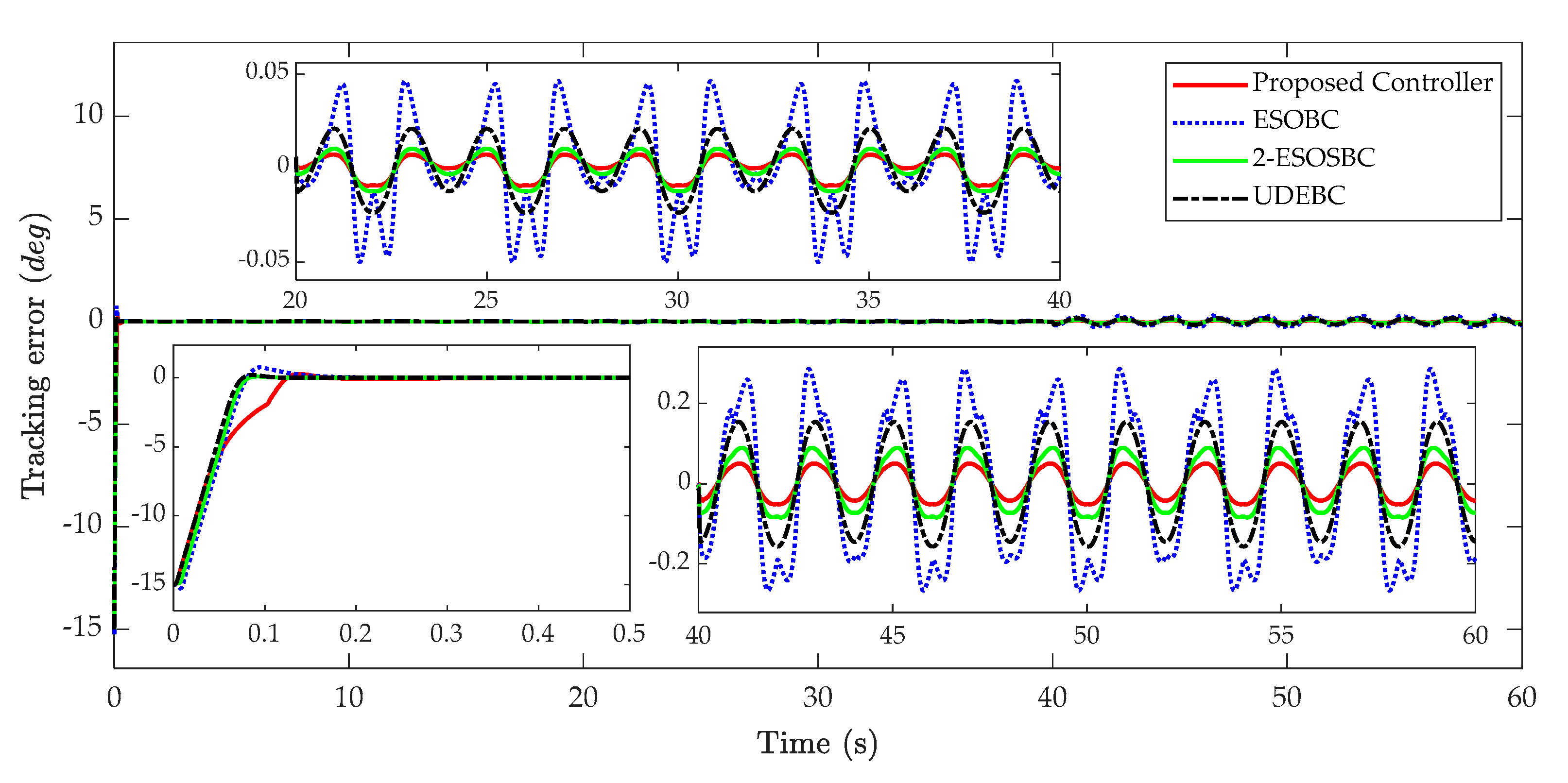
The tracking errors and tracking performances of four considered controllers are shown in Figure 4 and Figure 5, respectively. The maximum, average, and standard deviations of tracking errors in the steady-state phase are illustrated in

Table 2. The maximal absolute values of tracking error in the steady-state phase.

Control Approach	${\mathit{M}}_{\mathit{e}}\left(\mathbf{Deg}\right)$
	No Disturbance	Mismatched Disturbance	Mismatched/Matched Disturbances
Proposed Controller	0.0045	0.0093	0.0521
ESOBC Controller	0.0045	0.0500	0.2860
2-ESOBC Controller	0.0045	0.0123	0.0895
UDEBC Controller	0.0057	0.0236	0.1572

,

Table 3. The average tracking errors in the steady-state phase.

Control Approach	${\mathit{\mu }}_{\mathit{e}}\left(\mathbf{Deg}\right)$
	No Disturbance	Mismatched Disturbance	Mismatched/Matched Disturbances
Proposed Controller	0.0030	0.0048	0.0331
ESOBC Controller	0.0030	0.0219	0.1728
2-ESOBC Controller	0.0030	0.0065	0.0584
UDEBC Controller	0.0038	0.0131	0.0997

and

Table 4. The standard deviation of tracking errors in the steady-state phase.

Control Approach	${\mathit{\sigma }}_{\mathit{e}}\left(\mathbf{Deg}\right)$
	No Disturbance	Mismatched Disturbance	Mismatched/Matched Disturbances
Proposed Controller	0.0014	0.0030	0.0151
ESOBC Controller	0.0014	0.0189	0.1698
2-ESOBC Controller	0.0014	0.0038	0.0254
UDEBC Controller	0.0018	0.0068	0.0469

in detail, correspondingly.

In the absence of mismatched and matched disturbances in the first 20 s, the tracking performance and tracking error plots are roughly similar. The maximal absolute values of tracking errors of the proposed controller, ESOBC, and 2-ESOBC are 0.0045 degrees, whereas that of the UDEDC is slightly bigger with 0.0057 degrees.

In the presence of the mismatched lumped disturbance from the 20th second, the maximal value of tracking errors of the system with the ESOBC is significantly higher than other controllers with 0.05 degrees, because this mismatched term is only suppressed by using high gain feedback while this disturbance is estimated and compensated in other methods, while that of UDEBC is 0.0236 degrees. It can be seen from Table 2 that the tracking errors of the 2-ESOBC and proposed controller are better than the ESOBC and UDEBC, since the angular velocity and matched disturbance are approximated more precisely. In this case, the maximal absolute values of tracking errors of 2-ESOBC and the proposed method are 0.0123 degrees and 0.0093 degrees, respectively. This indicates that the proposed control approach achieves a better tracking performance than other approaches.

In the worst case, i.e., both mismatched and matched disturbances occur in the system from the 40th second, the tracking performances of all controllers deteriorate considerably. However, similar to the previous situation, it also illustrates the effectiveness of the proposed controller compared to the remaining controllers in the presence of both mismatched/matched uncertainties and external disturbances. In this case, the tracking performance of ESOBC and UDEBC is seriously deteriorated due to the effects of heavy disturbance with the maximum absolute values of the tracking errors being 0.2860 and 0.1572 degrees, respectively. Meanwhile, the maximal absolute value of tracking errors of 2-ESOBC is 0.08695 degrees, and the proposed controller has the most outstanding feature with this value is 0.0521 degrees under the effects of both mismatched and matched disturbances.

In addition, to evaluate the tracking performance of the compared methods in terms of smooth tracking performance, the average and standard deviation of tracking errors can be used. From Table 3 and Table 4, it can be observed that the average tracking error and standard deviation indexes of the proposed control algorithm are considerably smaller than other control approaches in the presence of mismatched and matched disturbances. They illustrate that the smoother tracking performance is achieved by the proposed method in comparison with others.

As above analysis, in the steady-state condition, the proposed controller achieves the best tracking performance in terms of steady-state tracking errors compared with other control methods, since the angular velocity of the actuator is estimated more accurately by employing Levant’s differentiator, and the matched/mismatched disturbances are also approximated then fed back to the controller to compensate for the effects of these disturbances on the control system.

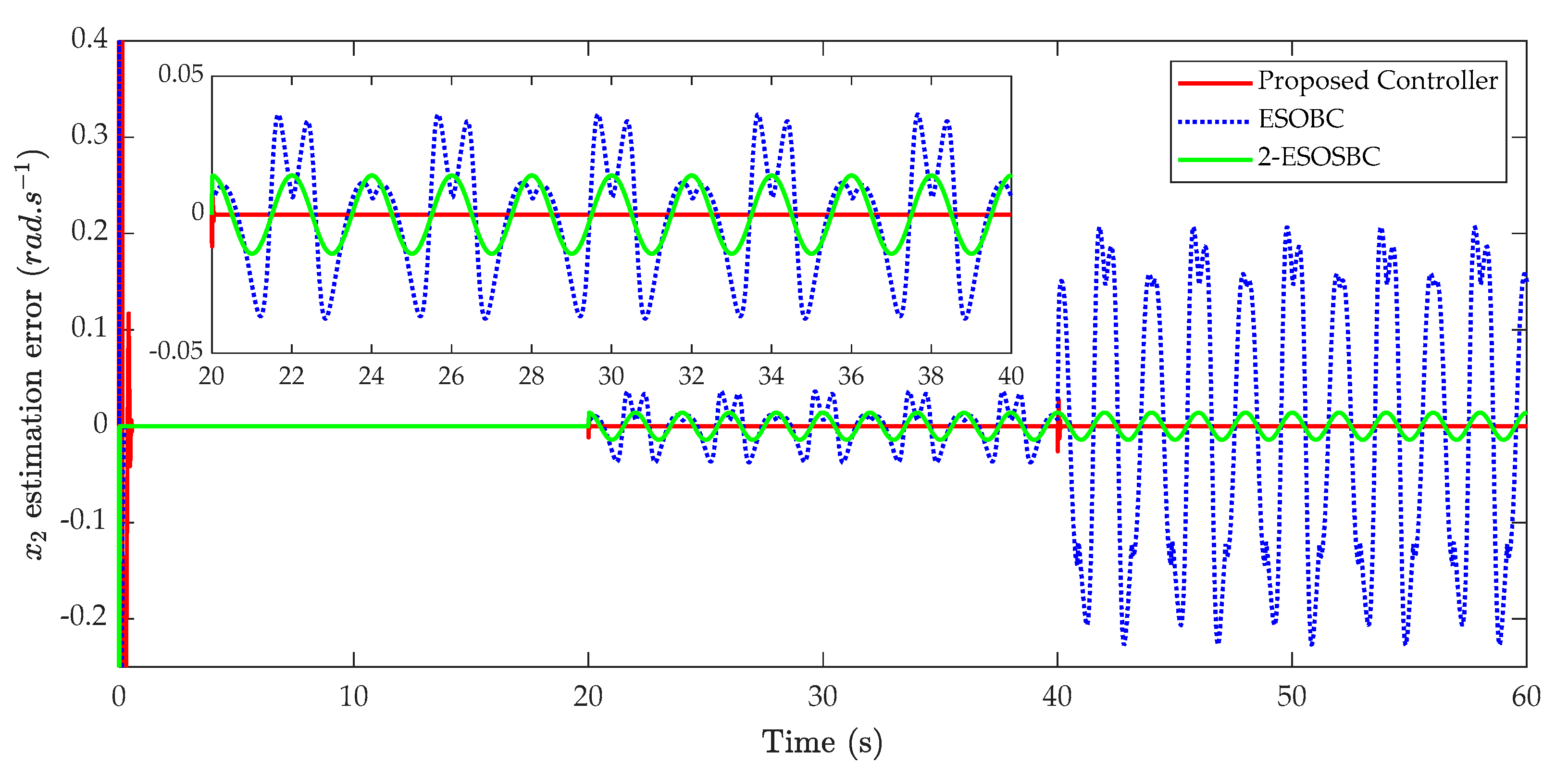
The estimation error of the angular velocity is depicted in Figure 6. It is immediately apparent that the angular velocity of the actuator is approximated by using the Levant’s differentiator much more exactly than using ESO [48]. It also can be seen from this figure, the estimation error of the 2ESOBC is much better than the ESOBC. In the occurrence of mismatched disturbance from the 20th second to 40th second, the velocity estimation errors of ESOBC and 2-ESOBC increase significantly, whereas that of the proposed controller remains unchanged. This error of ESOBC continues to enlarge dramatically under the influence of the matched disturbance in the last 20 s on the control system. Hence, the tracking performance of ESOBC deteriorates markedly under the presence of matched disturbance. An interesting point is observed that compared to the ESOBC, the angular velocity estimation in the 2-ESOBC is better since the pressure information is measured and fed back to the mismatched ESO which estimates the mismatched disturbance and also cancels its effect on the angular velocity estimation. In addition, based on the Levant’s differentiator, the angular velocity estimation in the proposed controller is the best compared to those in the remaining controllers because this estimation is independent of the system model and uncertainties/disturbances. Hence, it contributes to the best tracking performance in the above discussion as well as the best matched and mismatched disturbances estimations in the next section of the proposed controller compared to those of the remaining controllers.

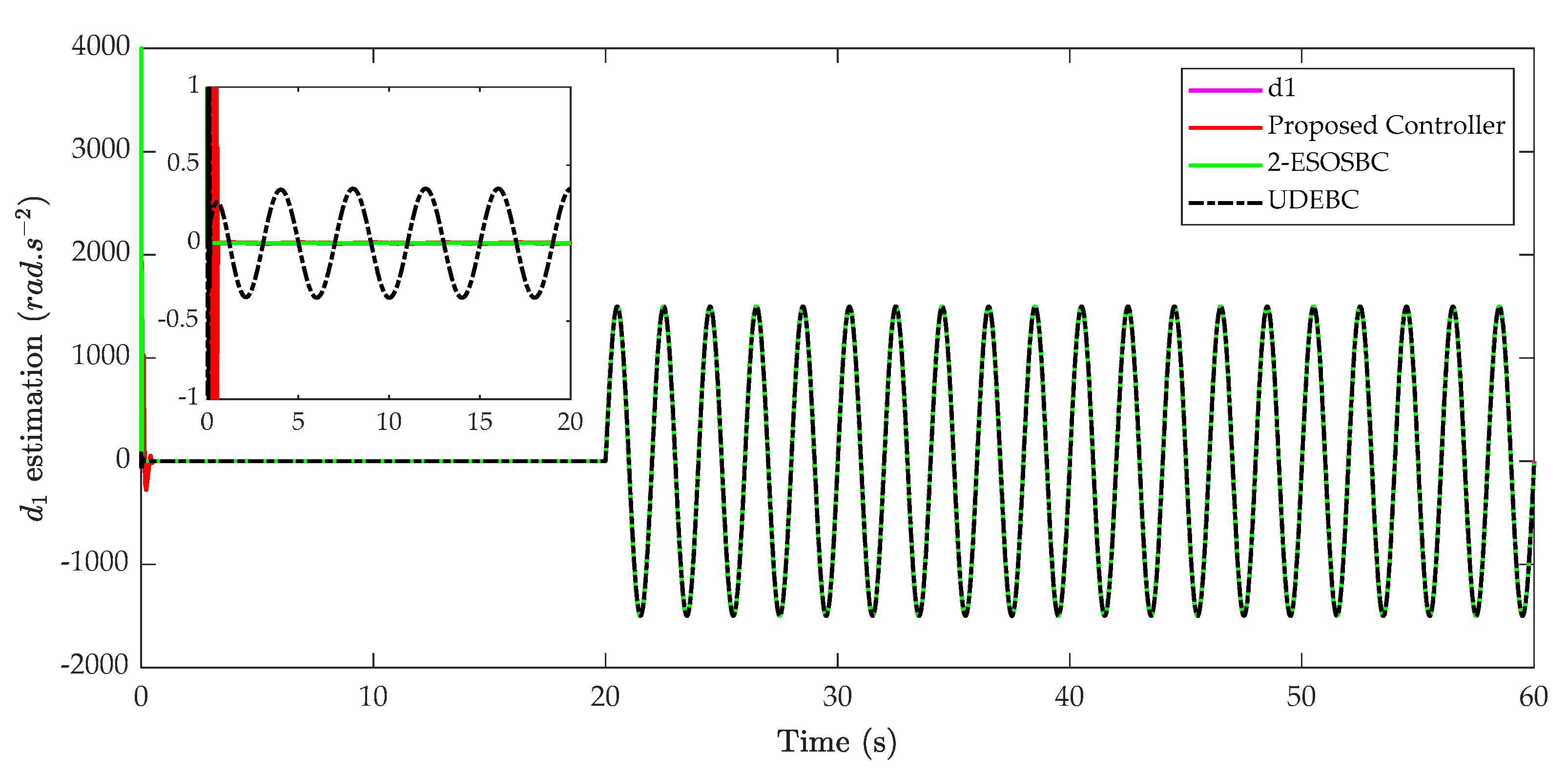
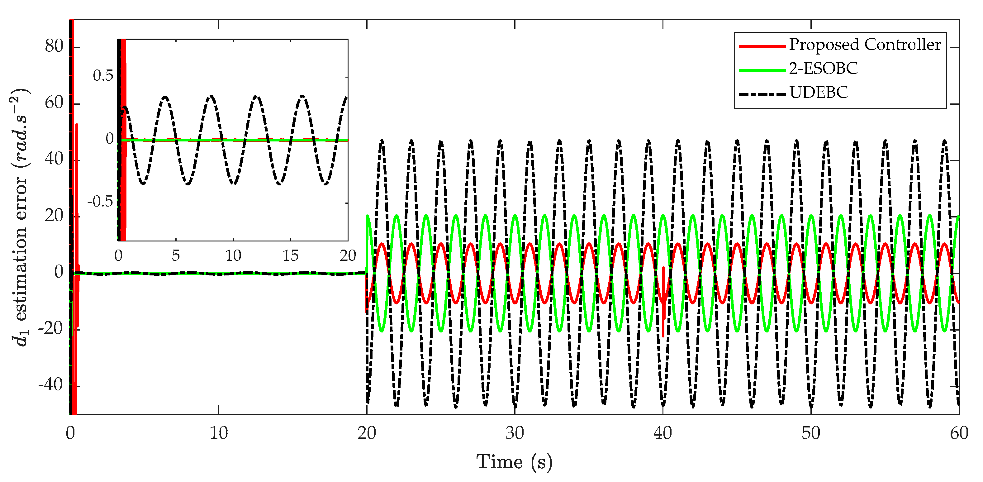
The estimation and estimation errors of mismatched disturbance are illustrated in Figure 7 and Figure 8. As shown in Figure 8, it is clearly seen that although the UDEBC can estimate the mismatched disturbance, the estimation error is considerably bigger than 2-ESOBC and the proposed method. From

Table 5. The maximal absolute value of estimation errors of mismatched and matched disturbances.

Control Approach	Maximal Value of Estimation Error
	Mismatched Disturbance $(\mathbf{rad}\cdot {\mathbf{s}}^{-2})$	Matched Disturbances $(\mathbf{rad}\cdot {\mathbf{s}}^{-3})$
Proposed Controller	16.3231	$1.1843\times {10}^4$
ESOBC Controller		$8.5159\times {10}^5$
2-ESOBC Controller	20.4977	$2.1428\times {10}^4$
UDEBC Controller	47.2756	$3.2072\times {10}^4$

, it can be observed that while the maximal absolute value of the mismatched estimation error of UDEBC is 47.2756 $\mathrm{rad}\cdot {\mathrm{s}}^{-2}$, those of 2-ESOBC and the proposed approach are 20.4977 $\mathrm{rad}\cdot {\mathrm{s}}^{-2}$ and 16.3231 $\mathrm{rad}\cdot {\mathrm{s}}^{-2}$, respectively. The results show that the proposed controller is able to estimate the mismatched disturbance the most accurately in comparison with UDEBC and 2-ESOBC.

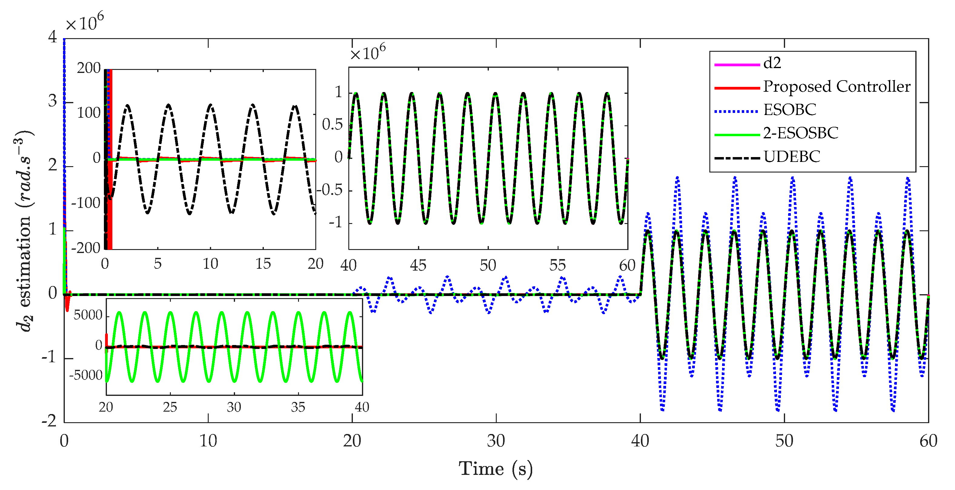
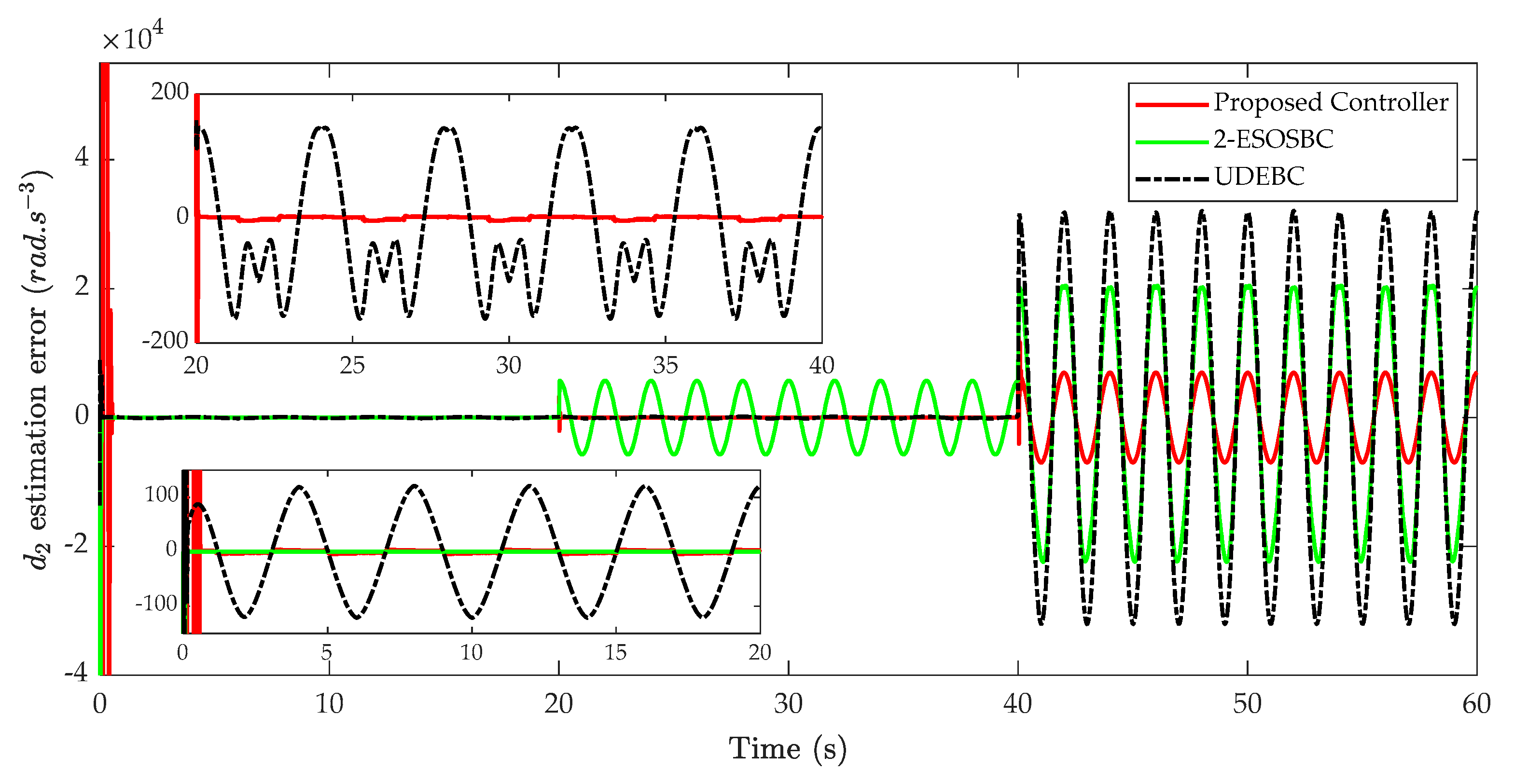
The estimation and estimation errors of matched disturbance are illustrated in Figure 9 and Figure 10. In Figure 10, the proposed disturbance observer is able to estimate more accurately the matched disturbance compared with other methods. It is worth noting that the matched disturbance estimation of the ESOBC and 2-ESOBC are affected by the mismatched disturbance due to the coupling problem between state and disturbance estimation. This leads the estimation errors even in the absence of matched disturbances, and hence, they degrade the tracking performance of the control system. Furthermore, the ESOBC uses high-gain feedback to suppress the matched disturbance, but in the case of heavy disturbance, this method cannot work well.

The maximal absolute values of matched disturbance of the estimation error are illustrated in Table 5. As can be seen from this table, the maximal absolute values of estimation error of ESOBC, UDEBC are 8.5159 × 10⁵ $\mathrm{rad}\cdot {\mathrm{s}}^{-3}$ and 3.2072 × 10⁴ $\mathrm{rad}\cdot {\mathrm{s}}^{-3}$, respectively, whereas these values of 2-ESOBC and the proposed method are 2.1428 × 10⁴ $\mathrm{rad}\cdot {\mathrm{s}}^{-3}$ and 1.1843 × 10⁴ $\mathrm{rad}\cdot {\mathrm{s}}^{-3}$, respectively.

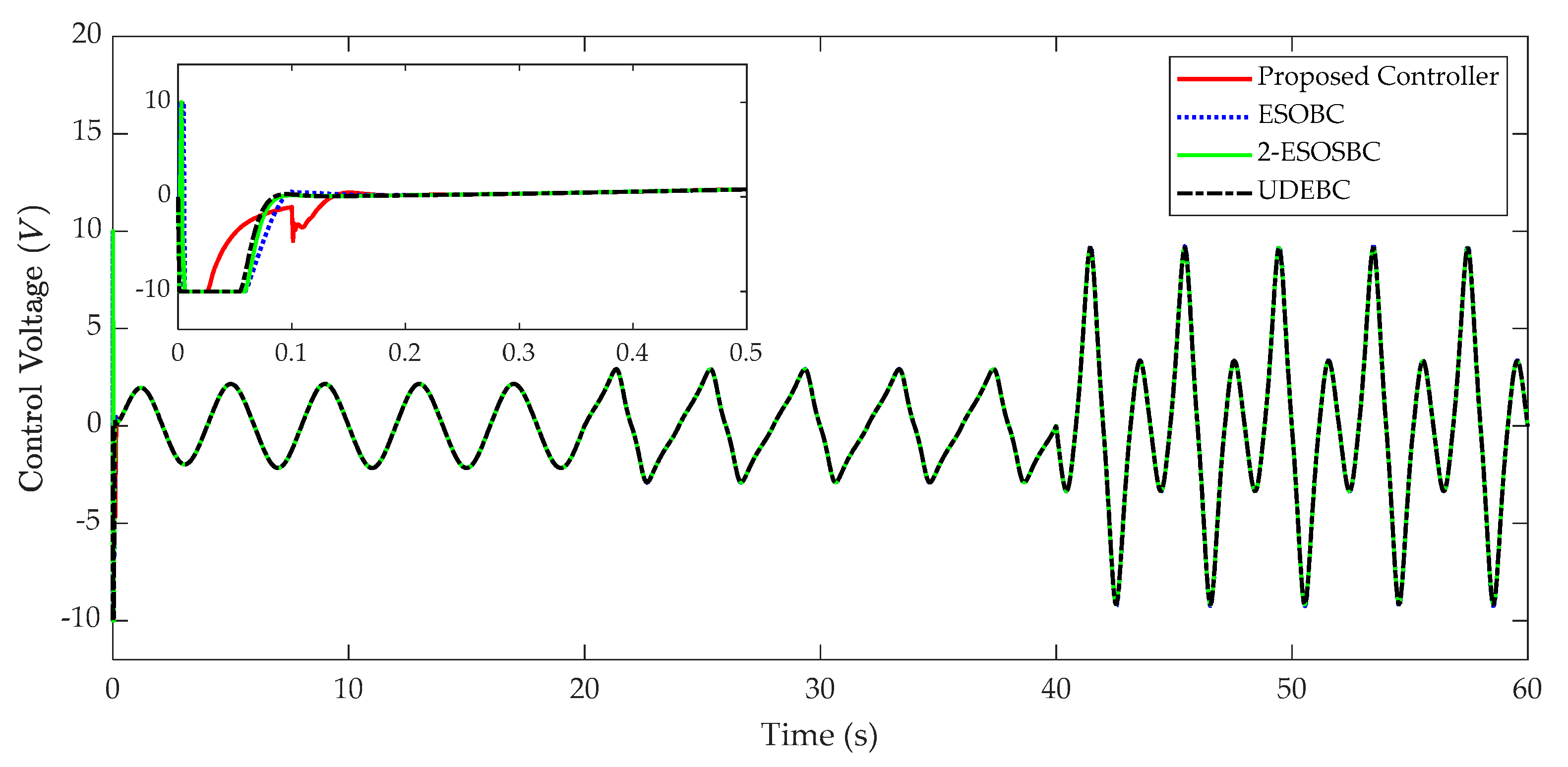
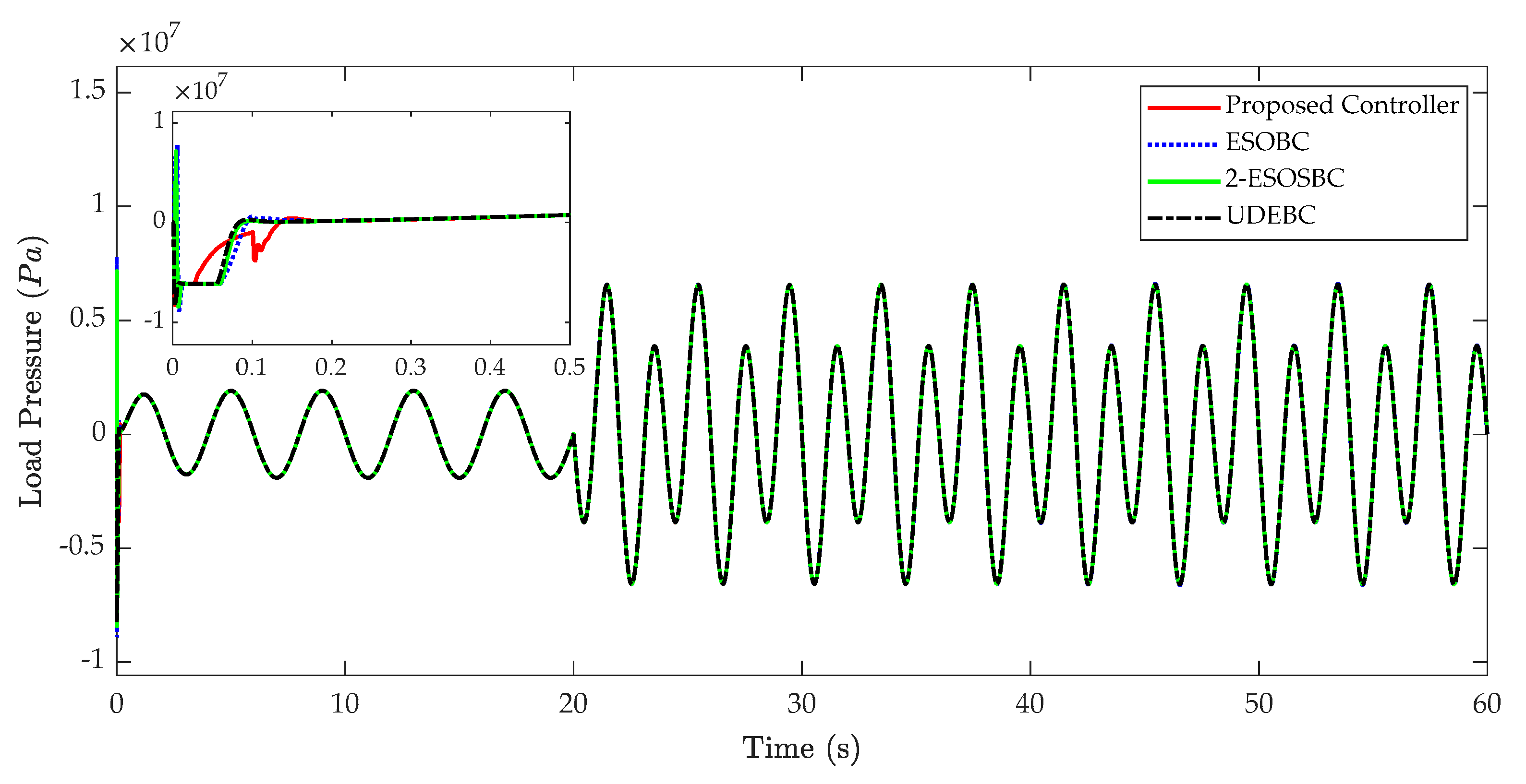
The control action and load pressures are shown in Figure 11 and Figure 12, respectively. Due to the same desired position trajectory and similar tracking performances, all four controllers generate the equivalent profiles of control input. It can be seen that in the presence of matched disturbance in the last 20 s, the value of control input increases significantly to compensate the effect of this uncertainty. The load pressure also changes to guarantee the tracking performance of the control system in the presence of mismatched and/or matched disturbances, and hence, the shapes of load pressures are also quite similar.

5. Conclusions

In this paper, a novel backstepping controller based on Levant’s differentiator-based disturbance observers has been proposed for a hydraulic servo-system. In this work, the angular velocity of the actuator is exactly estimated by employing the exact robust Levant’s differentiator. Lumped matched and mismatched disturbances are simultaneously considered and by using new DOs that approximate not only the uncertain nonlinearities but also the external disturbances. Based on that, the novel nonlinear controller is synthesized using the systematic backstepping method. The closed-loop system stability is completely proven using Lyapunov theory, which shows that the proposed controller guarantees a better tracking performance in the presence of time-varying uncertainties and external disturbances compared with other approaches. Comparative simulation results are attained to demonstrate the effectiveness of the proposed method. Future works include applying advanced nonlinear disturbance observers to improve the tracking performance and experiment validation on the real hydraulic system.