Fractional Control of a Lightweight Single Link Flexible Robot Robust to Strain Gauge Sensor Disturbances and Payload Changes

Abstract

In this paper, a method to control one degree of freedom lightweight flexible manipulators is investigated. These robots have a single low-frequency and high amplitude vibration mode. They hold actuators with high friction, and sensors which are often strain gauges with offset and high-frequency noise. These problems reduce the motion’s performance and the precision of the robot tip positioning. Moreover, since the carried payload changes in the different tasks, that vibration frequency also changes producing underdamped or even unstable time responses of the closed-loop control system. The actuator friction effect is removed by using a robust two degrees of freedom PID control system which feeds back the actuator position. This is called the inner loop. After, an outer loop is closed that removes the link vibrations and is designed based on the combination of the singular perturbation theory and the input-state linearization technique. A new controller is proposed for this outer loop that: (1) removes the strain gauge offset effects, (2) reduces the risk of saturating the actuator due to the high-frequency noise of strain gauges and (3) achieves high robustness to a change in the payload mass. This last feature prompted us to use a fractional-order PD controller. A procedure for tuning this controller is also proposed. Simulated and experimental results are presented that show that its performance overcomes those of PD controllers, which are the controllers usually employed in the input-state linearization of second-order systems.

1. Introduction

Robotic manipulators are used to assist in a wide range of tasks. Most of them are designed in such a way that the vibration of the end-effector is minimized in order to achieve good position accuracy. High tip position accuracy is achieved in industrial robots by endowing them with high structural stiffness, i.e., building them with links that are rigid can become simply rigid links. These robots are therefore heavy and bulky and are inefficient in terms of power consumption or speed of motion with regard to the operating payload [1]. Moreover, collision of this kind of robots cause remarkably destructive effects.

One effective solution by which to achieve high performance requirements such as high-speed operation, lower energy consumption, lighter weight and safer operation owing to reduced inertia, is to use robots which have slender lightweight links. Unfortunately, these building considerations, that lead to the mentioned advantages, reduce the stiffness of the structure of the link and cause serious vibration problems that substantially diminish the accuracy of the robot if they are not properly resolved. Links with low stiffness have also been applied in the medical field, such as for minimally-invasive surgery in which the endoscopic tools are mainly used. The flexibility of these medical devices allows them to follow tortuous paths with little interaction force with organs and with low risk of damaging tissues or causing pain to the patient, being therefore a safer mode [2]. The robots that have links with low stiffness are denoted flexible link robots (FLR). Controlling their behaviour has given rise to numerous problems in the field of dynamic modeling, control and sensory systems that have yet not been completely solved. A detailed list of these problems and the solutions achieved can be found in [3,4]. Some recent solutions to damp the vibrations of $FLR$ are: the control based on Port-Hamiltonian modeling [5], the sliding mode control [6], the adaptive control [7], the reinforcement learning control [8] and the fuzzy neural network control [9]. Moreover, multi-loop schemes have been used to control $FLR$ like in [10,11], in which the inner loop carried out the position control and the outer loop the vibration attenuation.

A $FLR$ robot has an infinite number of vibration modes. However, only a small number of modes is usually considered in the design of the control system. This number depends on the ratio between the links and the payload’ masses. Thus, the lower the ratio, the lighter the links and, furthermore, the heavier the payload, the smaller the number of significant vibration modes. Links made of composite materials (e.g., the graphite-epoxy or fiberglass) are able to carry heavy payloads though being very lightweight. Therefore, the large thin links made of these materials that are used in $FLR$ often have very small link-payload mass ratios and can be regarded as having a single vibration mode. This greatly simplifies the dynamic models of these robots and facilitates the design of their controllers. However, technically, there are several implementation problems of these controllers, which must be considered, and have not been satisfactorily solved yet:

(1)

Nonlinearities and time-varying parameters of the actuators reduce their performance: the discontinuous nonlinear Coulomb friction hinders the precise positioning of the robot tip, and the time-varying parameters as well as the actuator saturation produce overshoot and a slow response.

(2)

Strain gauges are often used as sensors in flexible link robots because they are cheap and measure both vibrations and deflections. However, strain gauges are prone to introduce two kinds of disturbances in the measurement: variations in temperature [4] produce a time-varying offset and electromagnetic interference produces high-frequency noise [12]. The first disturbance produces a steady-state error in the closed-loop position of the links [13]. The second disturbance may saturate the actuators, leading therefore to a bad dynamic behavior. Both disturbances dwindle the accuracy of the robot state observation (which is often needed for control) [14].

(3)

Robot tasks involve carrying variable payloads. Then, the control system has to be robust to these changes and must always preserve the stability, e.g., [15].

The first two problems have already been addressed in the context of active touch sensing using a robotic antenna with a flexible link. First, a control system for a single flexible link with a single degree of freedom ($1-DOF$) in the horizontal plane was developed in [16], which combined feedforward and feedback control. Later, this result was extended in [17] to a nonlinear robotic antenna with a single flexible link and two degrees of freedom ($2-DOF$) by applying the input-state feedback linearization technique [18]. In both papers, a control structure constituted by two nested loops was implemented:

(1)

An inner loop was closed around the actuators which fed back the actuator position. In this manner, a servo-controlled actuator robust to the Coulomb friction nonlinearity and viscous friction variations was achieved.

(2)

An outer loop in charge of removing the link vibrations was achieved feeding back the measurements of some strain gauges placed at the base of the flexible link. This outer loop removed the strain gauge offset, reduced the effects of sensor high-frequency noise and allowed to perform fast trajectories of the tip of the antenna without vibrations.

However, this control system presents two problems:

(1)

Robotic sensing antennae are not aimed to carry payloads. Then robustness to changing payloads was not addressed in the design of these controllers. Variations in the payload of $FLR$ produce changes in their vibration frequencies which may prompt underdamped or unstable responses in the closed-loop control system.

(2)

The outer loop controller is designed using frequency techniques and, in particular, phase margin and gain crossover frequency specifications. We found that these two specifications have to be chosen carefully because they may lead to control systems with two problems: (1) closed-loop poles that are canceled by zeros, which implies that the robot is able to accurately track a trajectory without vibrating but, in turn, it is not able to damp the vibrations caused by external disturbances, even in the case that only small changes are produced in the robot state and (2) unfulfillment of the desired time specifications because direct correspondences between them and frequency specifications only exist in the case of low order simple systems.

In order to cope with the first problem, this article proposes to use a fractional-order controller. These controllers are implemented using fractional order derivatives and can be often regarded as an extension of standard $PID$ controllers [19,20]. The robustness of these controllers to parametric changes has been extensively reported in the last two decades, e.g., [21]. In particular, several works can be found in the scientific literature about the design of fractional-order controllers robust to changes in the frequencies of mechanical vibrations. For example, a vehicle suspension system based on a fractional-order derivative controller ($FD$ controller) was developed in [22], a robust fractional strategy was developed for the speed control of a low-damped rotating multi-mass system in [23] and the control of systems with an arbitrary number of vibration modes whose frequencies can experience large changes was studied in [24]. Regarding manipulators, [25] proposed a fractional order fuzzy logic controller to control a rigid $2-DOF$ arm that experienced payload changes of $\pm 5\%$, and [26] applied a fractional-order sliding mode controller to a $FLR$ of $1-DOF$ that experienced payload changes of $\pm 25\%$. These last two articles developed relatively complex controllers, accepted small payload variations and reported only simulated results.

In order to cope with the second problem, this article proposes a method to design fractional-order controllers based on the closed-loop pole allocation technique. We will show that this technique allows us to design controllers with performances closer to the desired time specifications than the technique based on the frequency response.

Our control system proposal uses the above-mentioned two nested control loops scheme. It aims at solving the above-cited problems so that the performance and robustness of $FLR$ control systems is improved. It is focused on the control of a $FLR$ with a single link and $1-DOF$ that rotates in the horizontal plane. Moreover, it is assumed that the ratio between the link and the payload mass is low enough as to consider only one significant vibration mode. We will show that the commonly used $PD$ and $PID$ controllers cannot satisfy simultaneously the constraints introduced by the input-state feedback linearization technique and the robustness requirements and that, instead, a fractional-order $PD$ controller ($FPD$) can do it. Simulated and experimental results are provided that illustrate the advantages of the proposed controller and its tuning procedure.

The article is organized as follows. Section 2 describes the dynamic model of the $FLR$ to be controlled. Section 3 presents the control scheme, which is based on implementing two nested control loops. Section 4 exposes the new method proposed to tune the parameters of the controllers. Section 5 describes the experimental setup. Section 6 illustrates the simulations and experimental results obtained when implementing the $PD$ and the proposed $FPD$ controllers. Finally, Section 7 gives some conclusions.

2. Robot Dynamics

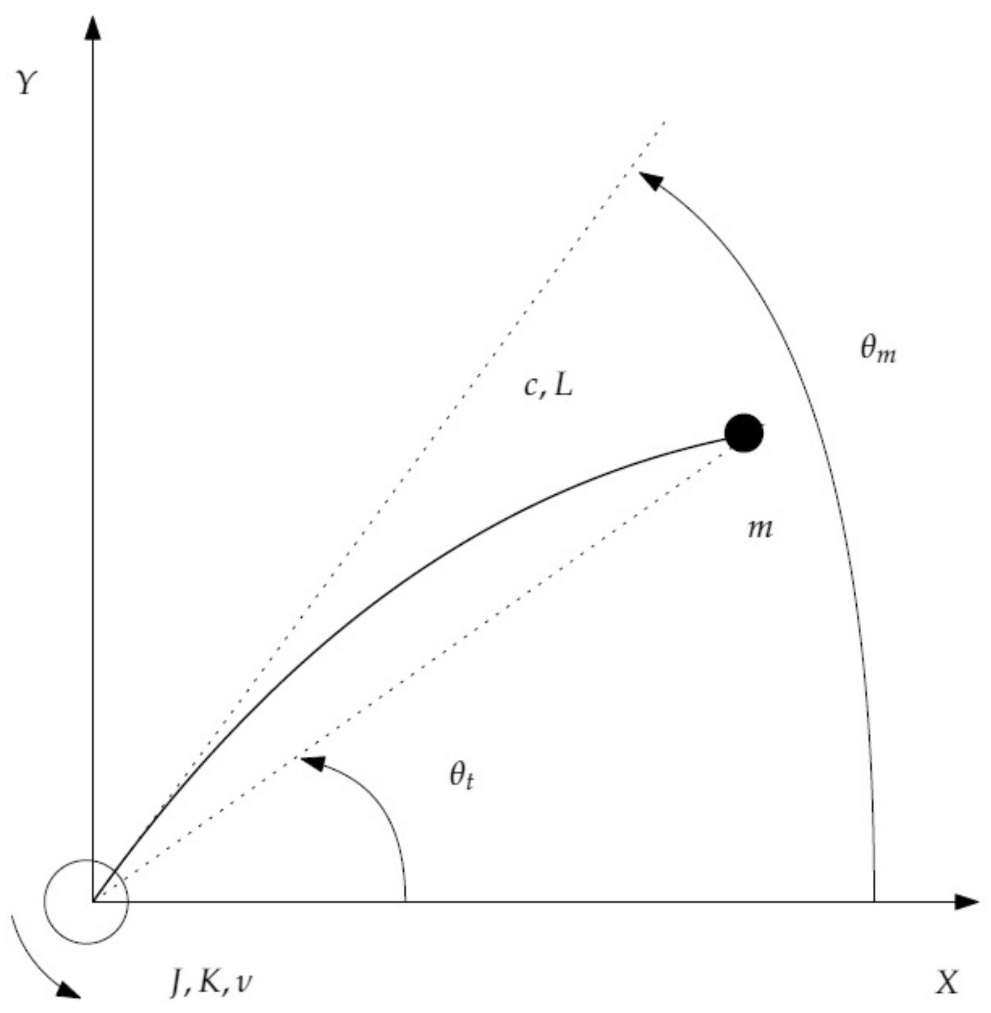
2.1. Flexible Link Dynamics

The dynamics of a single-link flexible manipulator carrying a payload is modeled. The payload is a disk attached to the robot tip through a vertical freely pivoted pin joint. Then the disk can freely rotate around its center of mass in the vertical axis, which implies that a negligible rotational moment is produced at the tip. The link is assumed to be an Euler–Bernoulli beam that has a small distributed mass. Axial deformation is neglected because the disk is floating on an air table that cancels the gravity effect and the friction of the disk with the table surface. Figure 1 shows the scheme of this setup. In this figure, ${\theta }_m$ rad is the joint angle, ${\theta }_t$ rad is the angle of the tip, i.e., the angular position of the payload, m is the payload mass, L is the length of the link, and $c=\frac{3·E·I}{L}$ is the stiffness of the link, where $E·I$ N·m${}^2$ is the flexural rigidity of the link.

Since structural damping usually increases the stability margin of the closed-loop control of an $FLR$, it is not included in the dynamic model developed here. A controller designed assuming a $FLR$ without damping is a conservative design that will remove the link vibrations even better if that damping existed.

Our study is carried out assuming the hypothesis of small deflections, which implies that the dynamics of the robot link can be regarded as linear. Since the mass of the disk is significantly larger than the mass of the beam, this last one can be neglected and we can assume that the vibration of the flexible beam has a single mode (the frequencies of the other modes are very far away from the first one and amplitudes associated with them are very small). Based on these considerations, the model for a $FLR$ proposed in [27] is used:

$$m·L^2·{\ddot{\theta }}_t=\mathrm{\Gamma }$$

(1)

which expresses the balance of torques at the base of the link. In this expression, $\mathrm{\Gamma }$ N·m is the moment transferred by the motor to the base of the link and $\ddot{{\theta }_t}$ rad/sec${}^2$ is the angular acceleration of the tip. This model is completed by the equation of the link deflection:

$$\mathrm{\Gamma }=c·({\theta }_m-{\theta }_t)$$

(2)

Combining (1) and (2) and taking Laplace transforms on the resulting equation, the transfer function between the tip and motor angles is obtained:

$$G\left(s\right)=\frac{{\theta }_t\left(s\right)}{{\theta }_m\left(s\right)}=\frac{{\overline{\omega }}^2}{s^2+{\overline{\omega }}^2}$$

(3)

where $\overline{\omega }$ is the fundamental frequency of our system, which is given by:

$$\overline{\omega }=\sqrt{\frac{c}{m·L^2}}$$

(4)

In these equations, the stiffness c is assumed to be perfectly known as well as L. However, the mass of the disk m may vary and, as consequence of the Equation (4), $\overline{\omega }$ varies too. Hereafter, we represent the nominal payload by $m_0$, the corresponding nominal frequency by ${\overline{\omega }}_0$ and the resulting nominal transfer function (3) by $G_0\left(s\right)$.

2.2. Rigid Dynamics

The rotational joint of the robot is actuated by a $DC$ motor. It is supplied by a servo-amplifier with a current inner loop control. The equation of the dynamics of this system can be obtained by using the Newton’s second law:

$$K·u=J·{\ddot{\theta }}_m+\nu ·{\dot{\theta }}_m+{\mathrm{\Gamma }}_c+\mathrm{\Gamma }$$

(5)

where K N·m/V is the electromechanical constant of the motor servo-amplifier system, J kg·m${}^2$ is the inertia of the motor, $\nu$ N·m·sec is the viscous friction coefficient, u V is the control signal, ${\ddot{\theta }}_m$ rad/sec${}^2$ and ${\dot{\theta }}_m$ rad/sec are, respectively, the angular acceleration and velocity of the motor, and ${\mathrm{\Gamma }}_c$ N·m is the Coulomb friction torque. This last nonlinear friction term is considered as a piecewise constant perturbation that depends only on the sign of the motor angular velocity:

$${\mathrm{\Gamma }}_c={\widehat{\mathrm{\Gamma }}}_c·sign\left({\dot{\theta }}_m\right)=\left\{\begin{array}{c}{\widehat{\mathrm{\Gamma }}}_c({\dot{\theta }}_m>0)\\ -{\widehat{\mathrm{\Gamma }}}_c({\dot{\theta }}_m<0)\end{array}\right\}$$

(6)

where ${\widehat{\mathrm{\Gamma }}}_c$ is the Coulomb friction constant. In the case that ${\dot{\theta }}_m=0$, the Coulomb friction is given by:

$${\mathrm{\Gamma }}_c=min\left(\left|K·u-\mathrm{\Gamma }\right|,{\widehat{\mathrm{\Gamma }}}_c\right)·sign\left(K·u-\mathrm{\Gamma }\right)$$

(7)

We note that Equations (5)–(7) are the equations of the motor referring to the output side of the gear, and that $\mathrm{\Gamma }$ can be regarded as the coupling torque between the motor and the flexible link.

The complete dynamics of the flexible link system actuated by the $DC$ motor can be therefore modeled by Equations (2)–(7). The input to this system is the voltage u applied to the motor and the output is the angular position of the payload ${\theta }_t$.

3. Control Scheme

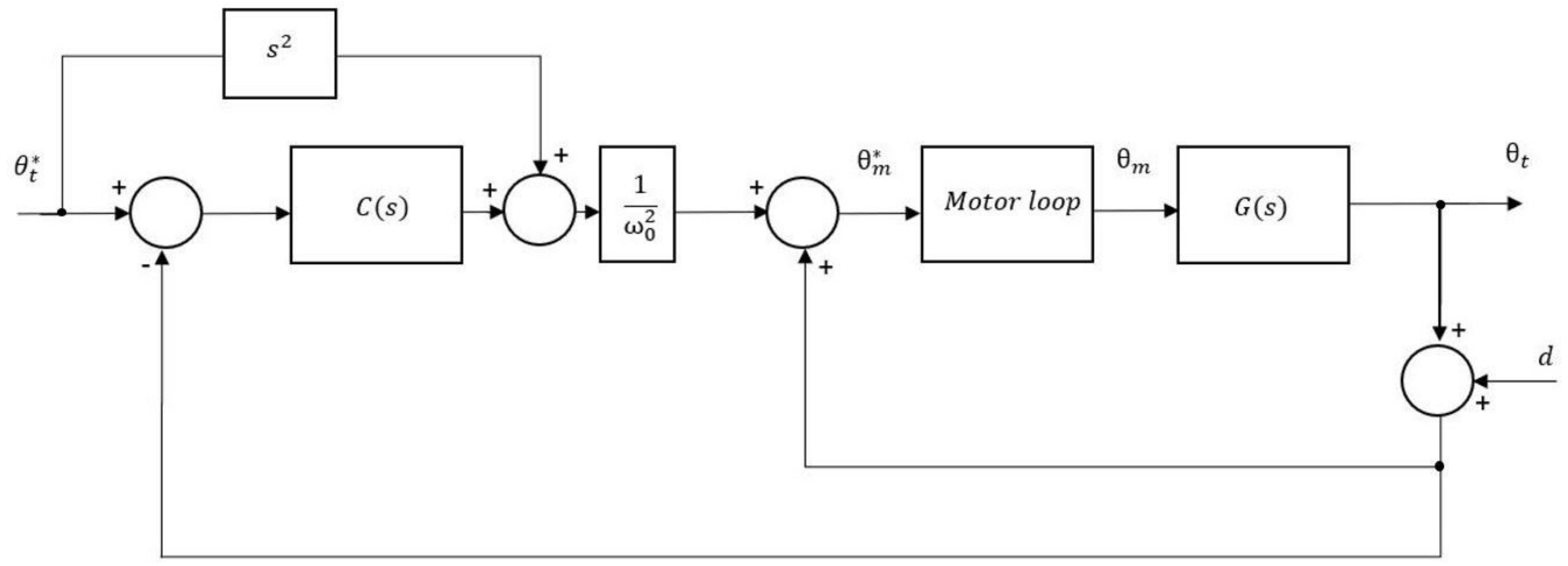
3.1. General Description

The controller of a $FLR$ feeds back the angle of the actuator ${\theta }_m$—which is often obtained using an optical encoder—and a measure of the link deflection, which is often the moment at the base of the link $\mathrm{\Gamma }$—which is measured using strain gauge bridges placed at the base of the flexible link [28].

This work uses the control scheme presented in [16,17], which implements two nested control loops:

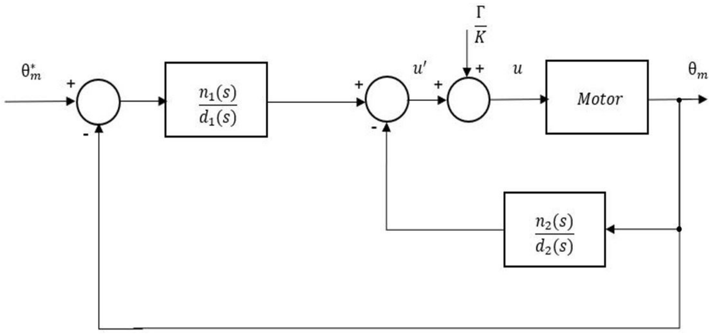
(1)

An inner loop that feeds back the measurement of the angle ${\theta }_m$ of the motor. This loop almost removes the effects of the nonlinear Coulomb friction and the time-varying viscous friction. Moreover, this loop is closed using a controller with high gains so that the dynamics of the resulting servo-controlled motor is much faster than the dynamics of the flexible link.

(2)

An outer loop that is in charge of controlling the position of the payload and moving it preventing the appearance of mechanical vibrations.

In this control scheme, the output of the control law of the outer loop is the reference of the inner loop. This strategy allows us to divide the design of the control system into two separate tasks. The motor is controlled in such a way that the fastest response allowed by its saturation levels is achieved. After that, the outer loop is designed using the singular perturbation theory, e.g., [18], that would allow us to neglect the dynamics of the inner loop if it were fast enough. The controller of the outer loop is tuned to achieve the desired tip positioning performance. The inner and outer loops are subsequently integrated into a singularly perturbed model and the stability of the whole system is studied.

3.2. Inner Loop Model

The control scheme presented in [17] is used here, which implements a two degrees of freedom robust $PID$ controller. The controller includes a feedback of the coupling torque which makes the dynamic of the controlled motor insensitive to the movements of the link. This feedback of the coupling torque clearly simplifies the motor model used to calculate the motor controllers. Next, this controller is outlined. The details of its design can be found in [29].

First, a fictitious control signal $u^{\prime }$ is defined as:

$$u^{\prime }\left(t\right)=u\left(t\right)-\frac{\mathrm{\Gamma }\left(t\right)}{K}$$

(8)

in order to cancel the effect of the link on the motor dynamics. Then Equation (5) becomes $K·u^{\prime }=J·{\ddot{\theta }}_m+\nu ·{\dot{\theta }}_m+{\mathrm{\Gamma }}_c$. Furthermore, if the Coulomb friction is assumed as a step-like disturbance to be compensated by the motor control loop, the dynamic model of the motor becomes linear being $K·u^{\prime }=J·{\ddot{\theta }}_m+\nu ·{\dot{\theta }}_m$, whose transfer function is:

$$\frac{{\theta }_m\left(s\right)}{u^{\prime }\left(s\right)}=G_m\left(s\right)=\frac{K}{s·(J·s+\nu )}$$

(9)

Based on model (9), a $PID$ controller with a low pass filter of the form:

$$\frac{n_1\left(s\right)}{d_1\left(s\right)}=\frac{a_2·s^2+a_1·s+a_0}{s·(s+c)}$$

(10)

is tuned, combined with a compensator:

$$\frac{n_2\left(s\right)}{d_2\left(s\right)}=\frac{b_1·s+b_0}{s+c}$$

(11)

in accordance with Figure 2. The closed-loop poles are allocated at desired locations following the procedure described in [29]. These four poles are placed on the same location z. Moreover, the two zeros of the closed-loop system are also placed on z. Then two of the four poles are cancelled by the two zeros yielding a simplified transfer function of the closed-loop system of the form:

$$\frac{{\theta }_m\left(s\right)}{{\theta }_m^{*}\left(s\right)}=M\left(s\right)=\frac{1}{{(1+ϵ·s)}^2},ϵ=-\frac{1}{z}$$

(12)

This control system ensures a good trajectory tracking, compensates disturbances such as unmodeled components of the friction, and is robust to parameter uncertainties. Such controller provides precise and fast positioning of the motor. Since very fast motor movements are required, $\left|z\right|$ is chosen as high as possible, and the value of $ϵ$ is therefore small.

3.3. Outer Loop Model

The outer control loop removes the link vibrations and its design involves the combination of the singular perturbation theory and the input-state linearization technique. We adapt here the nonlinear controller designed in [17] for a $2-DOF$ flexible sensing antenna to our $1-DOF$ linear $FLR$. In accordance with the singular perturbation theory, we design this controller assuming that $M\left(s\right)=1$, and then we check the stability of the closed-loop system with its complete dynamics including (12).

The transfer function of the system to be controlled is therefore $G\left(s\right)$ which is given by (3). Application of the input-state linearization technique to this linear system yields a control law of the form:

$${\theta }_m^{*}\left(s\right)={\theta }_t^{*}\left(s\right)+\frac{1}{{\overline{\omega }}_0^2}·(s^2·{\theta }_t^{*}\left(s\right)+C\left(s\right)·\left({\theta }_t^{*}\left(s\right)-{\theta }_t\left(s\right)\right))$$

(13)

where ${\theta }_t^{*}\left(s\right)$ is the trajectory desired for the payload, ${\theta }_m^{*}\left(s\right)$ is the control signal generated by the outer loop which, in turn, is the reference of the inner loop, ${\overline{\omega }}_0$ is the value of $\overline{\omega }$ in the case that the robot is carrying the nominal payload $m_0$, and $C\left(s\right)$ is the controller of the outer loop which, according to [18], must be a $PD$ controller of the form:

$$C\left(s\right)=k_p+k_d·s$$

(14)

in the case of controlling a second-order system (as it is the case of (3)). In this control law, the tip position ${\theta }_t$ is estimated from measurements of the motor angle ${\theta }_m$ and the strain gauges $\mathrm{\Gamma }$ equating ${\theta }_t$ in (2): ${\theta }_t\left(t\right)={\theta }_m\left(t\right)-\frac{\mathrm{\Gamma }\left(t\right)}{c}$. Assume that the measurement of the moment at the base of the link provided by the strain gauges has a disturbance $d^{\prime }\left(t\right)$ such that the estimated moment is ${\mathrm{\Gamma }}^e\left(t\right)=\mathrm{\Gamma }\left(t\right)+d^{\prime }\left(t\right)$. Thus, the estimation of ${\theta }_t$ becomes:

$${\theta }_t^e\left(t\right)={\theta }_m\left(t\right)-\frac{{\mathrm{\Gamma }}^e\left(t\right)}{c}={\theta }_m\left(t\right)-\frac{\mathrm{\Gamma }\left(t\right)}{c}+d\left(t\right)$$

(15)

where the disturbance $d\left(t\right)$ in the estimation of the tip position is $d\left(t\right)=-d^{\prime }\left(t\right)/c$. Figure 3 shows the scheme of the proposed control system including the sensor disturbance.

The transfer functions that relate the tip/payload angular position ${\theta }_t\left(t\right)$ and the control signal of the outer loop ${\theta }_m^{*}\left(t\right)$ with the reference ${\theta }_t^{*}\left(t\right)$ and the disturbance $d\left(t\right)$ are obtained after some operations:

$$\left(\begin{array}{c}{\theta }_t\left(s\right)\\ {\theta }_m^{*}\left(s\right)\end{array}\right)=\frac{\left(\begin{array}{cc}M\left(s\right)·G\left(s\right)·\frac{C\left(s\right)+s^2}{{\overline{\omega }}_0^2}& -M\left(s\right)·G\left(s\right)·\frac{C\left(s\right)-{\overline{\omega }}_0^2}{{\overline{\omega }}_0^2}\\ \frac{C\left(s\right)+s^2}{{\overline{\omega }}_0^2}& -\frac{C\left(s\right)-{\overline{\omega }}_0^2}{{\overline{\omega }}_0^2}\end{array}\right)}{1+M\left(s\right)·G\left(s\right)·\frac{C\left(s\right)-{\overline{\omega }}_0^2}{{\overline{\omega }}_0^2}}·\left(\begin{array}{c}{\theta }_t^{*}\left(s\right)\\ d\left(s\right)\end{array}\right)$$

(16)

and substituting (3) into this,

$$\left(\begin{array}{c}{\theta }_t\left(s\right)\\ {\theta }_m^{*}\left(s\right)\end{array}\right)=\underset{Q\left(s\right)}{\underbrace{\frac{\left(\begin{array}{cc}{\left(\frac{\overline{\omega }}{{\overline{\omega }}_0}\right)}^2·M\left(s\right)·\left(C\left(s\right)+s^2\right)& -{\left(\frac{\overline{\omega }}{{\overline{\omega }}_0}\right)}^2·M\left(s\right)·\left(C\left(s\right)-{\overline{\omega }}_0^2\right)\\ \frac{\left(C\left(s\right)+s^2\right)·\left({\overline{\omega }}^2+s^2\right)}{{\overline{\omega }}_0^2}& -\frac{\left(C\left(s\right)-{\overline{\omega }}_0^2\right)·\left({\overline{\omega }}^2+s^2\right)}{{\overline{\omega }}_0^2}\end{array}\right)}{s^2+{\overline{\omega }}^2+{\left(\frac{\overline{\omega }}{{\overline{\omega }}_0}\right)}^2·M\left(s\right)·\left(C\left(s\right)-{\overline{\omega }}_0^2\right)}}}·\left(\begin{array}{c}{\theta }_t^{*}\left(s\right)\\ d\left(s\right)\end{array}\right)$$

(17)

3.4. Achieving Robustness to Strain Gauge Disturbances

Two kind of disturbances may appear in a strain gauge signal: offset and high frequency noise. In this Section, the controllers proposed in [16,17] for reducing their effects are adapted to our $1-DOF$$FLR$.

3.4.1. Offset Elimination

Consider the transfer function of (17) that relates ${\theta }_t\left(s\right)$ and $d\left(s\right)$:

$$\frac{{\theta }_t\left(s\right)}{d\left(s\right)}=Q_{1,2}\left(s\right)=-{\left(\frac{\overline{\omega }}{{\overline{\omega }}_0}\right)}^2·\frac{M\left(s\right)·\left(C\left(s\right)-{\overline{\omega }}_0^2\right)}{s^2+{\overline{\omega }}^2+{\left(\frac{\overline{\omega }}{{\overline{\omega }}_0}\right)}^2·M\left(s\right)·\left(C\left(s\right)-{\overline{\omega }}_0^2\right)}$$

(18)

Since the offset can be modeled as a step disturbance $d\left(s\right)=\widehat{d}/s$, the steady state error $e_{{\theta }_t}$ caused in ${\theta }_t$ by this disturbance can be assessed applying the final value theorem, e.g., [30]:

$$e_{{\theta }_t}=\underset{s\to 0}{lim}s·Q_{1,2}\left(s\right)·d\left(s\right)=-{\left(\frac{\overline{\omega }}{{\overline{\omega }}_0}\right)}^2·\frac{M\left(0\right)·\left(C\left(0\right)-{\overline{\omega }}_0^2\right)}{{\overline{\omega }}^2+{\left(\frac{\overline{\omega }}{{\overline{\omega }}_0}\right)}^2·M\left(0\right)·\left(C\left(0\right)-{\overline{\omega }}_0^2\right)}·\widehat{d}$$

(19)

Taking into account that $M\left(0\right)=1$, this expression yields that $C\left(0\right)$ must be ${\overline{\omega }}_0^2$ in order to make $e_{{\theta }_t}=0$. Then controllers of the form:

$$C\left(s\right)=\widehat{C}\left(s\right)+{\overline{\omega }}_0^2,\widehat{C}\left(0\right)=0$$

(20)

, i.e., with the term $\widehat{C}\left(s\right)$ having a zero in the origin, completely remove the steady state error caused by the offset.

3.4.2. Reduction of the Effect of the High Frequency Noise

The high frequency noise of the sensor produces an amplified noise in the control signal ${\theta }_m^{*}\left(t\right)$ that may produce actuator saturation. This yields a deficient dynamic performance and even instability.

Consider now the transfer function of (17) that relates ${\theta }_m^{*}\left(s\right)$ and $d\left(s\right)$:

$$\frac{{\theta }_m^{*}\left(s\right)}{d\left(s\right)}=Q_{2,2}\left(s\right)=-\frac{1}{{\overline{\omega }}_0^2}·\frac{\left(C\left(s\right)-{\overline{\omega }}_0^2\right)·\left({\overline{\omega }}^2+s^2\right)}{s^2+{\overline{\omega }}^2+{\left(\frac{\overline{\omega }}{{\overline{\omega }}_0}\right)}^2·M\left(s\right)·\left(C\left(s\right)-{\overline{\omega }}_0^2\right)}$$

(21)

Assuming a controller of the form (20) we have that:

$$Q_{2,2}\left(s\right)=-\frac{1}{{\overline{\omega }}_0^2}·\frac{\widehat{C}\left(s\right)·\left({\overline{\omega }}^2+s^2\right)}{s^2+{\overline{\omega }}^2+{\left(\frac{\overline{\omega }}{{\overline{\omega }}_0}\right)}^2·M\left(s\right)·\widehat{C}\left(s\right)}$$

(22)

The high frequency noise of the strain gauge signal can be modeled by a sinusoidal signal of very high frequency. Then the frequency response of $Q_{2,2}$ at $\omega \to \infty$ shows how the effect of this noise on the control signal ${\theta }_m^{*}$ of the outer loop is amplified. Dividing the numerator and denominator of $Q_{2,2}\left(s\right)$ by $s^2$ yields that:

$$\underset{\omega \to \infty }{lim}\left|Q_{2,2}(j·\omega )\right|=\frac{1}{{\overline{\omega }}_0^2}·\underset{\omega \to \infty }{lim}\frac{|\widehat{C}(j·\omega )|·\left|1-\frac{{\overline{\omega }}^2}{{\omega }^2}\right|}{\left|1-\frac{{\overline{\omega }}^2}{{\omega }^2}-{\left(\frac{\overline{\omega }}{{\overline{\omega }}_0}\right)}^2·\frac{M(j·\omega )·\widehat{C}(j·\omega )}{{\omega }^2}\right|}$$

(23)

Let us assume that:

$$\underset{\omega \to \infty }{lim}\frac{|\widehat{C}(j·\omega )|}{{\omega }^4}=\psi <\infty$$

(24)

Then ${lim}_{\omega \to \infty }\left|\frac{M(j·\omega )·\widehat{C}(j·\omega )}{{\omega }^2}\right|=\psi /{ϵ}^2$ and consequently:

$$\underset{\omega \to \infty }{lim}\left|Q_{2,2}(j·\omega )\right|=\frac{1}{{\overline{\omega }}_0^2}·\frac{{lim}_{\omega \to \infty }\left|\widehat{C}(j·\omega )\right|}{\left|1-{\left(\frac{\overline{\omega }}{{\overline{\omega }}_0}\right)}^2·\frac{\psi }{{ϵ}^2}\right|}$$

(25)

This expression shows that the effect of the high frequency noise on the control signal ${\theta }_m^{*}\left(t\right)$ is highly reduced if:

$$\underset{\omega \to \infty }{lim}\left|\widehat{C}(j·\omega )\right|=0$$

(26)

We note that (26) guarantees the verification of condition (24). Condition (26) means that the order of the numerator of $\widehat{C}\left(s\right)$ must be lower than the order of the denominator.

Remark 1.

Since the inner loop includes controllers with high gains, the effect on the motor input $u\left(t\right)$ of a high frequency noise in ${\theta }_m^{*}\left(t\right)$ is highly amplified, being thus prone to saturating the motor. Then condition (26) has to be necessarily verified in order to prevent this effect.

4. Control Robust to Payload Changes

Changes in the payload m produce changes in the vibration frequency $\overline{\omega }$ in accordance with (4). Changes of this frequency produce underdamped or even unstable closed-loop systems. This section develops a controller $C\left(s\right)$ that, embedded in the control scheme described in Section 3, provides a robust behavior to payload changes. This controller must be also robust to strain gauge offset and high frequency noise. Then $C\left(s\right)$ must verify conditions (20) and (26).

4.1. A Fractional-Order Controller

Since the dynamics of the inner loop (12) is much faster than the dynamics of the link (3), the following analysis is carried out applying the singular perturbation theory, e.g., [18]. It is then assumed that $M\left(s\right)=1$ and the characteristic equation of the closed-loop system—which is the denominator of (17)—becomes:

$$s^2+{\overline{\omega }}^2+{\left(\frac{\overline{\omega }}{{\overline{\omega }}_0}\right)}^2·\widehat{C}\left(s\right)=0$$

(27)

It can be expressed as:

$$1+\frac{{\overline{\omega }}^2}{s^2+{\overline{\omega }}^2}·\frac{\widehat{C}\left(s\right)}{{\overline{\omega }}_0^2}=0$$

(28)

Next we recall a result about achieving isophase margin robustness of oscillatory systems [24]: given an oscillator (3) in which $\overline{\omega }$ has a large uncertainty, it can be robustly controlled in the sense of achieving a phase margin invariant to $\overline{\omega }$ changes—it is denoted the isophase margin property—by closing a loop using a fractional-order controller of the form:

$$\widehat{C}\left(s\right)=k_f·s^{\alpha },\alpha \in {\Re }^{+},0<\alpha <2$$

(29)

This controller was designed in [24] using the phase margin and gain crossover frequency specifications.

Controller (29) is improper. Several structures of fractional-order $PID$ controllers have been proposed [31] to make proper these controllers. In particular, the phase-lead fractional-order controller [32] is the proper realization of the $FPD$ controller. In our case, since we need that $\widehat{C}\left(s\right)$ has a zero in the origin in order to preserve the offset effect cancellation and $\alpha$ can be higher than one, we modify controller (29) to:

$$\widehat{C}\left(s\right)=k_f·\frac{s^{\alpha }}{\left(1+\mu ·s\right)}$$

(30)

in order to make it strictly proper.

Frequency specifications do not have an easy interpretation in terms of time specifications. Then this section proposes a new method to tune controllers (29), (30) by applying a closed-loop pole allocation technique. Since the controller structure is preserved in this method, the isophase margin property will be maintained.

The final step of the controller design using the singular perturbation theory requires checking the range of values $ϵ$ of $M\left(s\right)$ that make stable the closed-loop system. Theorem 11.4 from the book [18] is often used to carry out this study. However, this theorem was developed only for integer-order systems. Some researchers have tried to extend the singular perturbation theory to fractional order systems [33] and have applied it to the $PID$ control of nonlinear systems [34]. We recall here the recent extension of the mentioned theorem of [18] to fractional-order nonlinear systems [35], which would allow us to apply the singular perturbation theory to our control system.

4.2. Dynamic Specifications

Let us assume that $0<\alpha <2$ in (29). Then the characteristic Equation (27) has two poles $p_1$ and $p_2$. In order to be able to apply the singular perturbation technique, these two poles must be much closer to the imaginary axis than the double pole z of $M\left(s\right)$. We impose then an ‘a priori’ condition to the relative position between these two pairs of poles:

$$|real\left(p_1\right)|,|real\left(p_2\right)|<|z|/5$$

(31)

in order to be able to apply that technique. In any case, the stability of the complete closed-loop system will have to be verified ‘a posteriori’.

Let us assume that the two desired closed-loop poles $p_1$ and $p_2$ are complex conjugates. They are expressed in polar form as $p_{1,2}=p·e^{\pm j\varphi }$. We use two time specifications to determine these two poles: the settling time $t_s$ and the overshoot $M_p$. In the case of an underdamped second-order system, the previous specifications are related to the position of the poles in the complex plane by the expressions:

$$t_s\approx \frac{\pi }{\sigma }$$

(32)

$$M_p=e^{\frac{-\pi \xi }{\sqrt{1-{\xi }^2}}},\xi =cos\left(\theta \right)$$

(33)

where the meaning of parameters $\sigma$ and $\theta$ is shown in Figure 4. These specifications are desired for the nominal process ${\overline{\omega }}_0$. In this case, $\overline{\omega }={\overline{\omega }}_0$, and the characteristic Equation (27) becomes:

$$s^2+{\overline{\omega }}_0^2+\widehat{C}\left(s\right)=s^2+C\left(s\right)=0$$

(34)

4.3. Tuning the Controller

We need controllers that have at least two parameters to be tuned in order to be able to achieve the two specifications defined above. Substituting $s=p_1$ or $s=p_2$ in Equation (34) yields two simple conditions that allow us to tune the parameters of the controller.

In the following, we carry out the design of four simple controllers with two or more tunable parameters:

(1)

PD controller: $C_{PD}\left(s\right)=k_p+k_d·s$. This controller has two parameters to be tuned. Then the dynamic specifications can be achieved but not the robustness to strain gauges offset nor the robustness to payload changes. In this case, (34) becomes $s^2+k_d·s+k_p=0$, and substituting $s=p_1$ yields:

$$p^2·e^{j·2·\varphi }+k_d·p·e^{j·\varphi }+k_p=0\Rightarrow \left\{\begin{array}{c}{k}_p=p^2\\ k_d=-2·p·cos\left(\varphi \right)\end{array}\right.$$

(35)

(2)

FPD controller: $C_{FPD}\left(s\right)={\overline{\omega }}_0^2+k_f·s^{\alpha }$. This controller has three parameters to be tuned. Then the dynamic specifications can be achieved as well as the robustness to strain gauges offset. Moreover, the structure of this controller yields the iso phase margin property to changes in the payload. In this case, (34) becomes $s^2+k_f·s^{\alpha }+{\overline{\omega }}_0^2=0$, and substituting $s=p_1$ yields:

$$p^2·e^{j·2·\varphi }+k_f·p^{\alpha }·e^{j·\alpha ·\varphi }+{\overline{\omega }}_0^2=0\Rightarrow \left\{\begin{array}{c}\alpha =\frac{\angle -{\overline{\omega }}_0^2-p^2·e^{j·2·\varphi }}{\varphi }\\ k_f=\frac{|{\overline{\omega }}_0^2+p^2·e^{j·2·\varphi }|}{p^{\alpha }}\end{array}\right.$$

(36)

(3)

Proper FPD controller: $C_{P-FPD}\left(s\right)={\overline{\omega }}_0^2+k_f·\frac{s^{\alpha }}{{(1+\mu ·s)}^2}$. This controller has four parameters to be tuned. In this case, the dynamic specifications can be achieved as well as the robustness to strain gauges offset. The structure of this controller yields an isophase margin property to payload changes which is not as good as that of the previous controller. In any case, if the gain crossover frequency ${\omega }_c$ of the system varies in the range ${\omega }_{cl}\le {\omega }_c\le {\omega }_{ch}$ as consequence of changes in the payload, choosing a value:

$$\mu <\frac{1}{5·{\omega }_{ch}}$$

(37)

and the same values of $k_f$ and $\alpha$ as in $C_{FPD}\left(s\right)$ assures that $C_{P-FPD}(j·\omega )\approx C_{FPD}(j·\omega )$ in the mentioned frequency range, and the isophase margin property becomes guaranteed for the range of variation of the payload. Since controller (30) is proper (always $\alpha <2$), $C_{P-FPD}\left(s\right)$ reduces the effect of the high frequency noise in the control signal ${\theta }_m^{*}\left(t\right)$. In this case, (34) becomes $s^2+k_f·\frac{s^{\alpha }}{{(1+\mu ·s)}^2}+{\overline{\omega }}_0^2=0$, and the tuning procedure is carried out in five steps:

(a)

Obtain controller $C_{FPD}\left(s\right)$ from expression (36).

(b)

Calculate the range of gain crossover frequencies $[{\omega }_{cl},{\omega }_{ch}]$ for the previous $C_{FPD}\left(s\right)$.

(c)

Choose a value of $\mu$ using condition (37).

(d)

Obtain controller $C_{P-FPD}\left(s\right)$ using the previous value of $\mu$. In this case, (34) becomes $s^2+k_f·\frac{s^{\alpha }}{{(1+\mu ·s)}^2}+{\omega }_0^2=0$, and substituting $s=p_1$ yields:

$$p^2·e^{j·2·\varphi }+k_f·\frac{p^{\alpha }·e^{j·\alpha ·\varphi }}{{(1+\mu ·p·e^{j·\varphi })}^2}+{\overline{\omega }}_0^2=0\Rightarrow \left\{\begin{array}{c}\alpha =\frac{\angle -\left({\overline{\omega }}_0^2+p^2·e^{j·2·\varphi }\right)·{(1+\mu ·p·e^{j·\varphi })}^2}{\varphi }\\ k_f=\frac{|{\overline{\omega }}_0^2+p^2·e^{j·2·\varphi }|·|1+\mu ·p·e^{j·\varphi }{|}^2}{p^{\alpha }}\end{array}\right.$$

(38)

(e)

Check that the gain crossover frequency range $[{\omega }_{cl},{\omega }_{ch}]$ obtained with $C_{P-FPD}\left(s\right)$ verifies condition (37). If not, a lower value of $\mu$ has to be chosen and the procedure has to be repeated until a satisfactory controller is found.

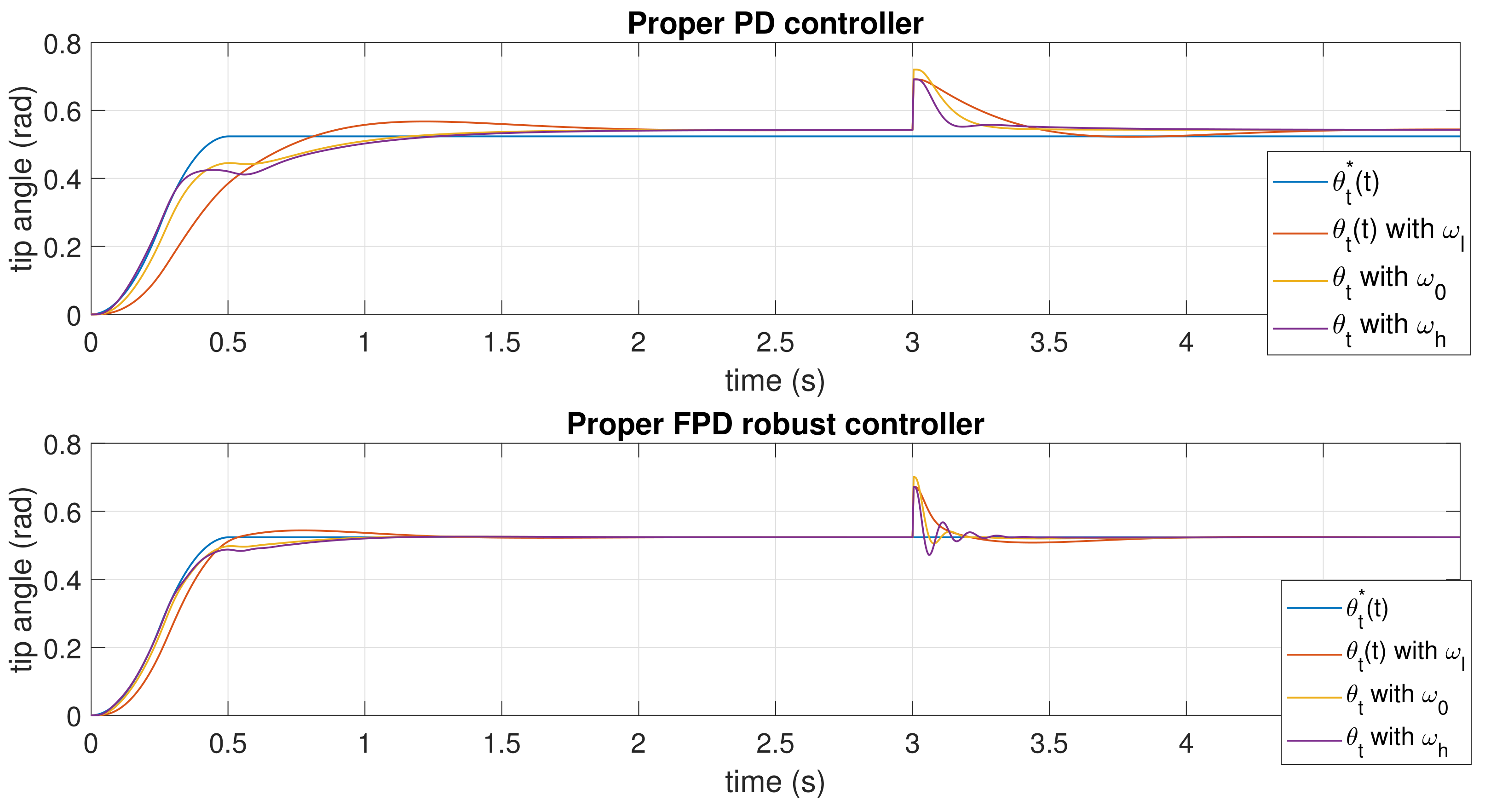
(4)

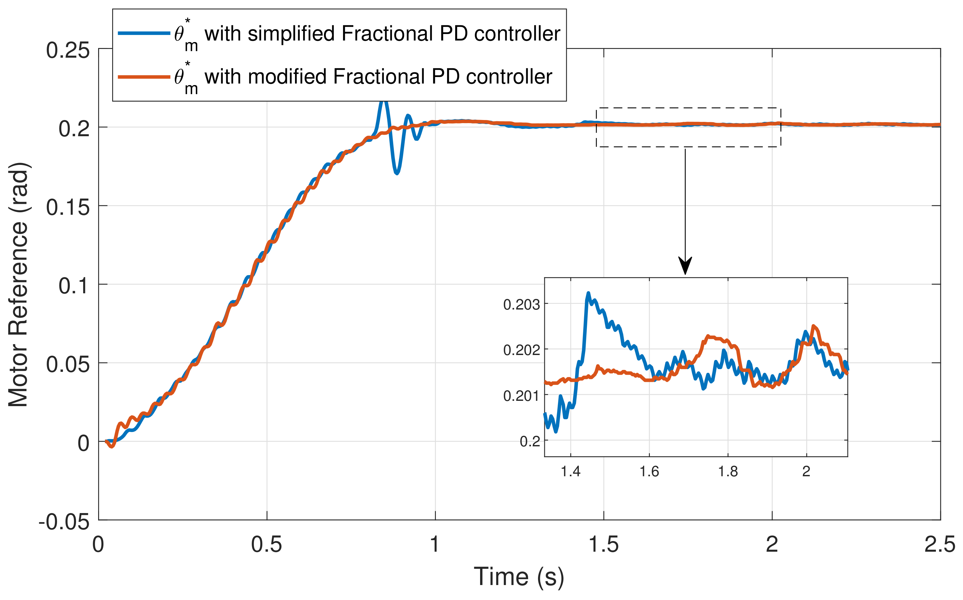
Proper PD controller: $C_{P-PD}\left(s\right)=k_p+k_d·\frac{s}{{(1+\mu ·s)}^2}$. This controller has three parameters to be tuned. It uses the same values $k_p$ and $k_d$ designed for $C_{PD}\left(s\right)$ but the derivative term is modified by adding the same filter as in the $C_{P-FPD}\left(s\right)$ in order to attain a similar attenuation of the high-frequency noise. Since $\mu$ is low, the double pole introduced at $-1/\mu$ has a small influence on the values of the two dominant poles $p_1$ and $p_2$ of the closed-loop system.

Remark 2.

The procedure to design the Proper FPD controller always converges to a satisfactory solution. However, it must be taken care of the obtained μ. In some cases, it may be too low to really reduce the effect of the high-frequency noise of the strain gauges in the control signal. If the value of μ were unsatisfactory, the controller must be redesigned changing a specification (a time specification or relaxing the accuracy required in the verification of the isophase margin robustness).

The final step of the controller design procedure, which is based on the theorem of [18] for singularly perturbed nonlinear systems, can be simplified in our case because we have an $FLR$ whose dynamics is linear. In this case, we can apply the well-known root locus method to assess the location of the poles of the complete system when parameter $\mathsf{\lambda }={\left(\frac{\overline{\omega }}{{\overline{\omega }}_0}\right)}^2$ varies. The denominator of (17) gives the following closed-loop characteristic equation:

$$s^2+{\overline{\omega }}^2+{\left(\frac{\overline{\omega }}{{\overline{\omega }}_0}\right)}^2·M\left(s\right)·\left(C\left(s\right)-{\overline{\omega }}_0^2\right)=0$$

(39)

and rearranging:

$$1+\mathsf{\lambda }\frac{{\overline{\omega }}_0^2+M\left(s\right)·\left(C\left(s\right)-{\overline{\omega }}_0^2\right)}{s^2}=0$$

(40)

which can be used to plot the root locus of both the simplified and the complete systems.

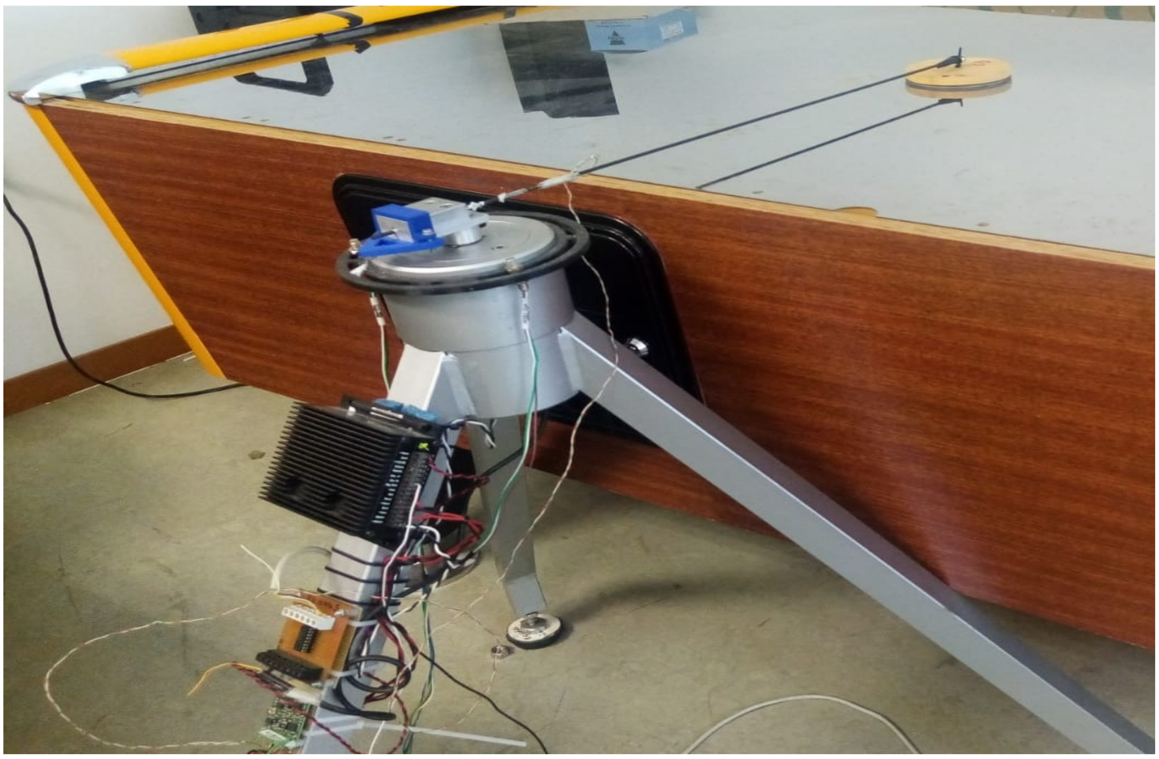
5. Experimental Platform

5.1. Setup Description

Figure 5 is a picture of the experimental platform, which is constituted by a three legged metallic structure that supports a Harmonic Drive mini servo DC motor $RH-8D-6006-E036AL-SP\left(N\right)$ that has a reduction ratio characterized by $n=50$. This frame makes it possible the stably and free rotation of the motor in the horizontal plane around the vertical axis of the platform. The motor parameter values are: inertia $J=6.87\times {10}^{-5}$ kg·m${}^2$, viscous friction $\nu =1.041\times {10}^{-3}$ N·m·sec and electromechanical constant $K=0.21$ N·m/V. The servo-amplifier accepts control inputs from the computer in the range of $[-10,10]$ V. The flexible beam is attached to the motor. The load (disk) floats over the surface of an air table in such a way that the friction with the surface of the table and the gravity effect are canceled. The flexible beam characteristics are: length $L=0.5$ m, diameter $d=3\times {10}^{-3}$ m, flexural rigidity $EI=0.260$ N·m${}^2$ and $c=3·EI/L=1.56$ N·m. The nominal tip load is a wood disk of mass $m_0=0.05$ kg. Then the nominal vibration frequency of the link is characterized as ${\overline{\omega }}_0=10.99$ rad/sec ($f_0=1.75$ Hz). Other two disks of masses $m_l=0.0312$ kg and $m_h=0.1249$ kg are used, whose respective vibration frequencies are ${\overline{\omega }}_l=7.1226$ rad/sec ($f_l=1.132$ Hz) and ${\overline{\omega }}_h=14.2463$ rad/sec ($f_h=2.2674$ Hz). The sensor system consists of an encoder embedded in the motor—which allows us to know the motor angular position with a precision of $7\times {10}^{-5}$ rad—and a pair of strain gauges with gauge factor $2.16$ and resistance $120.2$$\Omega$. The sampling time of the signals processing is 4 msec.

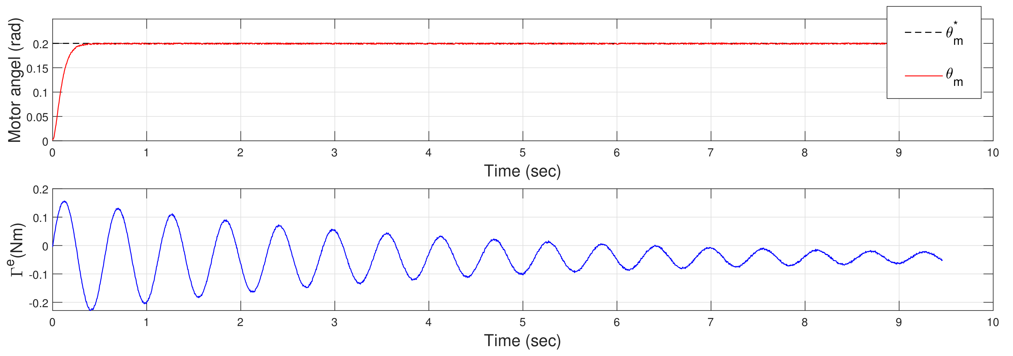
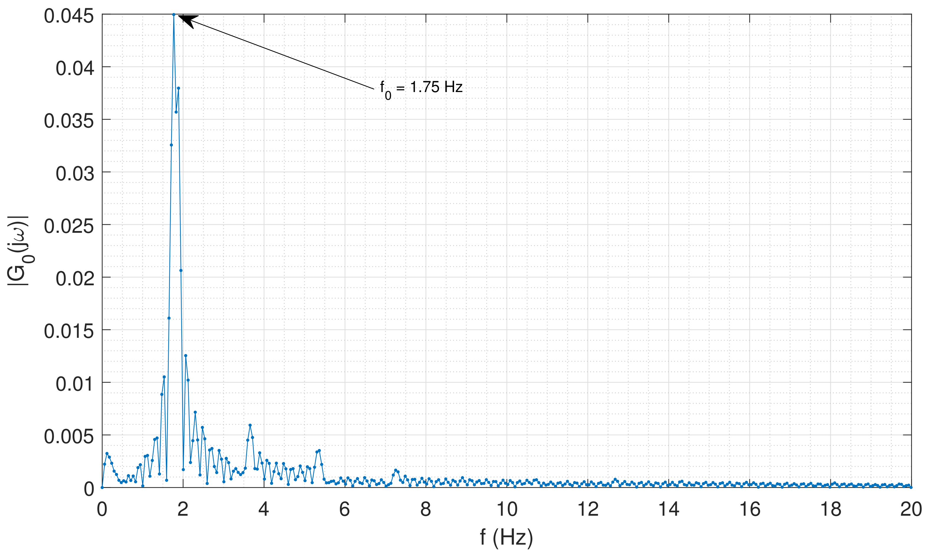
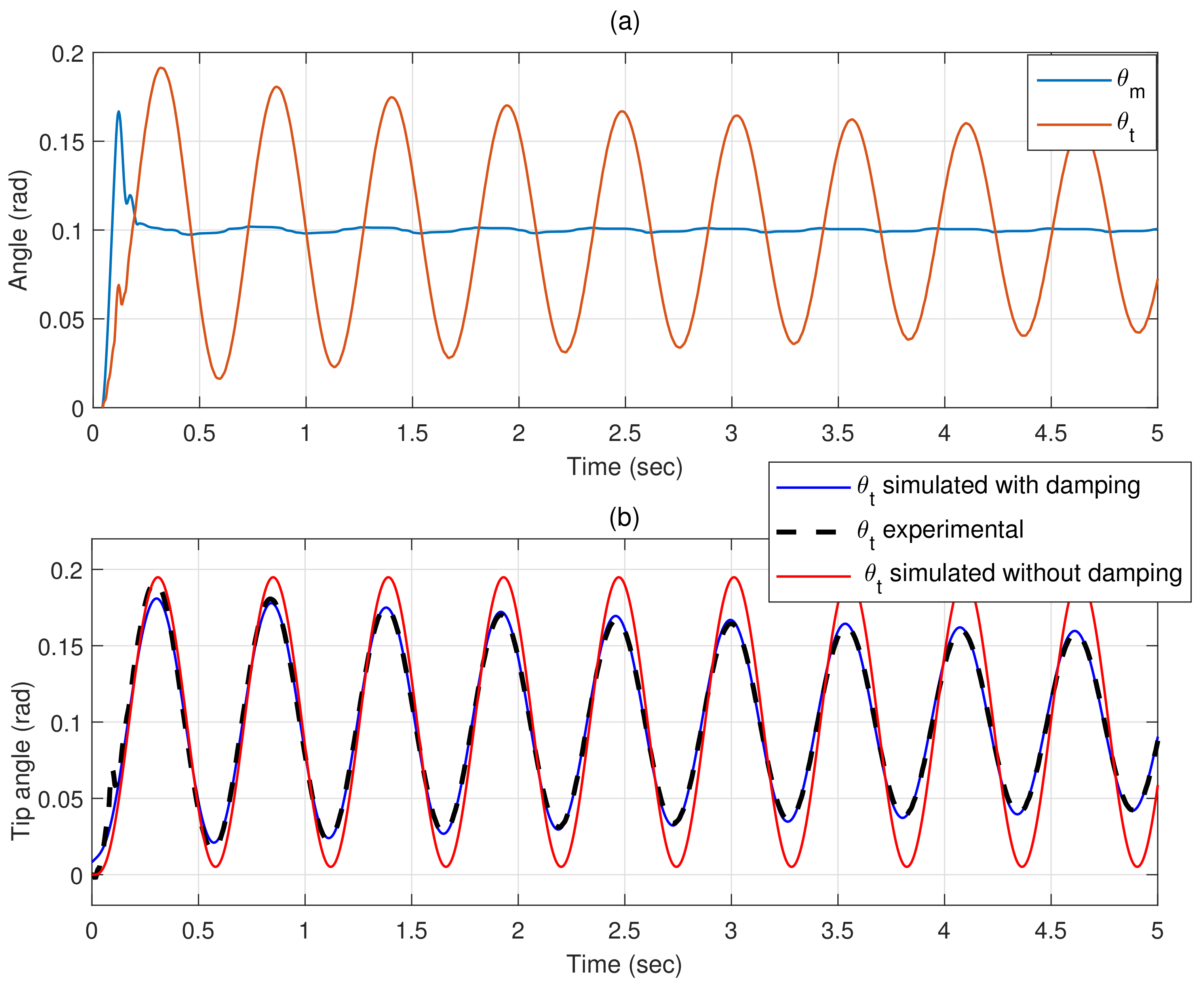
5.2. Setup Dynamics Validation

The dynamics of the flexible robot was characterized by studying its frequency response. It was obtained by applying a chirp signal to the input ${\theta }_m^{*}\left(t\right)$ of the inner loop, having disconnected the outer loop. The angle of the motor ${\theta }_m\left(t\right)$ and the moment at the base of the link $\mathrm{\Gamma }\left(t\right)$ were recorded, and the $FFT$s of these two signals were calculated. The quotient of these $FFT$s gave the frequency response of the link. Figure 6 is a periodogram that shows the magnitude of the frequency response in the case of carrying the nominal disk. This figure shows a single peak. Then there is a single vibration mode. Moreover, that peak is observed at a frequency $f_0=1.75$ Hz (${\overline{\omega }}_0=10.99$ rad/seg), which is exactly the value estimated from the link parameters using (4). All this supports the assumptions that the link is massless, all the mass is concentrated at the tip of the link and the rotation moment produced at the tip is zero.

Figure 7 shows the response to a step command applied at the input of the inner loop. The upper figure shows the reference step ${\theta }_m^{*}\left(t\right)$ and the motor angle response ${\theta }_m\left(t\right)$, and the lower figure shows the measurement of the moment at the base of the link provided by the strain gauges ${\mathrm{\Gamma }}^e\left(t\right)$. The upper figure shows that, in the steady-state after the maneuver, the motor angle is resting in the reference position. Since there is no deflection in the steady-state because the link moves in an horizontal plane (the gravity does not produce any moment), the measurement of the moment at the base of the link should oscillate around zero. However, the signal of the lower figure oscillates noticeably around a negative value showing that the strain gauges signal has a significant offset in the steady-state. This prompts us to design controllers robust to this measurement disturbance.

Finally, Figure 8 shows the response to an abrupt command applied at the input of the inner loop when the robot carries the nominal disk. Figure 8a shows the motor angle response ${\theta }_m\left(t\right)$ measured by the encoder and the tip angle response ${\theta }_t\left(t\right)$ estimated from measurements of the motor encoder and the strain gauges using (15). This Figure 8a shows that the link has a slight damping: in the steady state of the motor, where its angle shows a very small residual vibration, the amplitude of the oscillation of the tip angle is slightly decreasing. Then Figure 8b shows again the experimental tip response ${\theta }_t\left(t\right)$ (black dashed line), the simulated tip response provided by the undamped model (3) with $\overline{\omega }={\overline{\omega }}_0=10.99$ rad/s obtained from the previous frequency response characterization (red line), and the simulated tip response provided by a damped model:

$$G_d\left(s\right)=\frac{{\theta }_t\left(s\right)}{{\theta }_m\left(s\right)}=\frac{{\overline{\omega }}^2}{s^2+2·\zeta ·\overline{\omega }·s+{\overline{\omega }}^2}=\frac{125.44}{s^2+0.1484·s+125.44}$$

(41)

which has been fitted between the tip response ${\theta }_t\left(t\right)$ and the motor response ${\theta }_m\left(t\right)$ using the Identification Toolbox of $MATLAB$ (the blue line). The parameters of (41) yielded by this identification procedure were $\overline{\omega }=11.2$ rad/s and $\zeta =0.006$. We remark that the red and blue plots of Figure 8b are the simulated time responses of models (3) and (41) when the input is the motor angle shown in Figure 8a. The error between the theoretical vibration frequency (which coincides with the value estimated using the frequency response of Figure 6) and the vibration frequency obtained by the identification based on the time responses is $1.91\%$, which allows us to consider that the theoretical value ${\overline{\omega }}_0=10.99$ rad/s adequately reproduces the oscillation (the experimental response and the red line response show approximately the same frequency and phase in Figure 8b). Moreover, the estimated damping coefficient is very small, which allows us to neglect it and use the undamped model (3).

6. Control System Validation

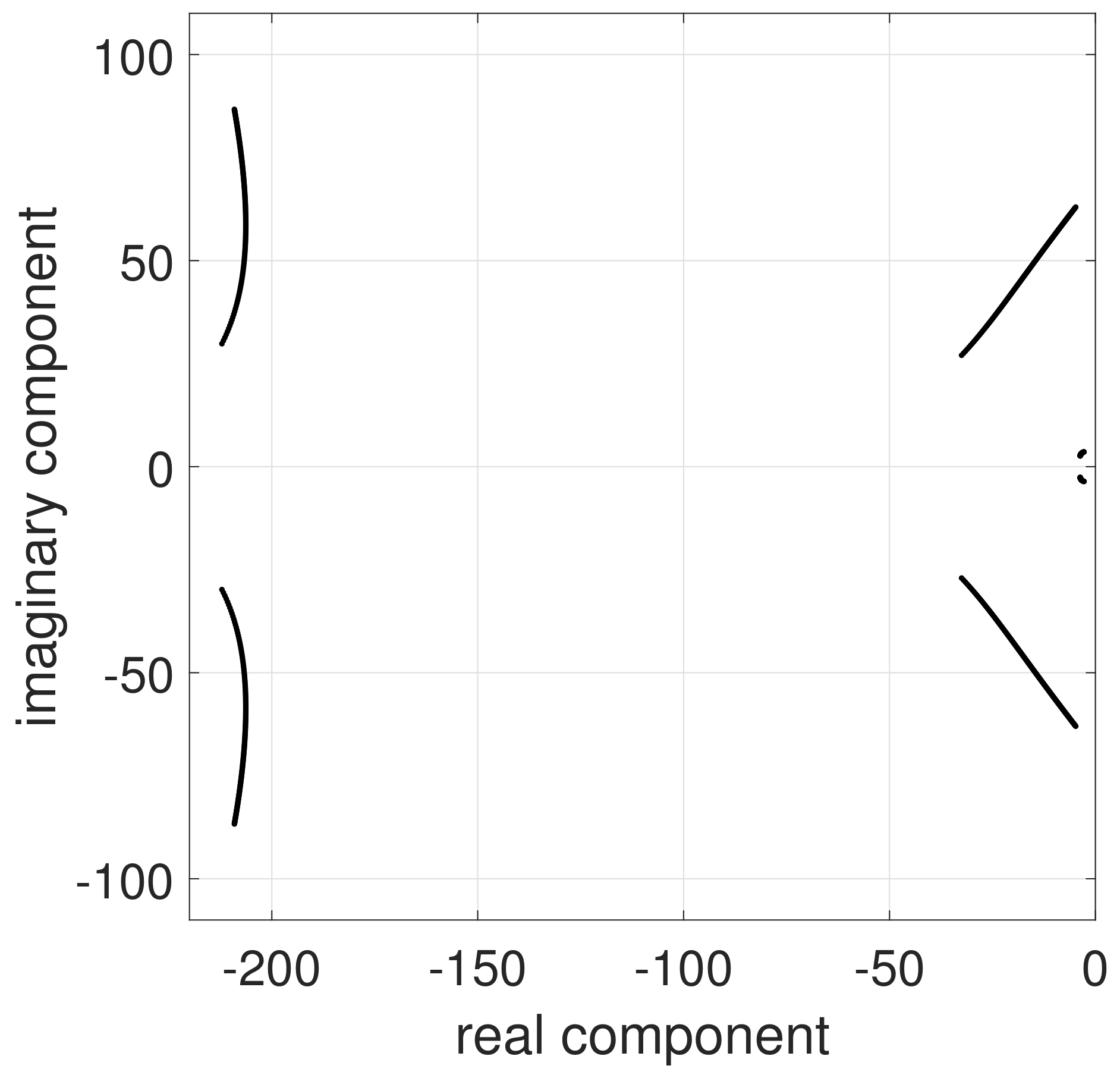
6.1. Design of the Control System

The inner loop is designed using the procedure described in [29] with the motor parameters listed in Section 5.1. The two poles of the inner loop are placed in $z=-80$.

Proper $PD$ and $FPD$ controllers are designed for the outer loop. Two time specifications are used to tune the parameters of these controllers: the settling time $t_s$ which must be lower than 1 sec, and an overshoot $M_p$ which must be lower than $5\%$. In the case of an under-damped second order system such as ours, expressions (32) and (33) can be applied. Then choosing $\theta =\frac{\pi }{4}$ rad and $p=5$ yields that $\varphi =2.356$ rad, $\xi =0.7071$, $\sigma =p·cos\left(\theta \right)=3.5354$, $M_p=4.32\%<5\%$ and $t_s=\frac{\pi }{\sigma }=0.8886<1$. Therefore, the closed-loop poles of the outer loop are placed at $p_{1,2}=5·e^{\pm j·2.356}$. Note also that condition (31) needed to apply the singular perturbation technique is verified: $\left|real\right(p_{1,2}\left)\right|=\sigma =3.5354<<\left|z\right|/5=16$.

Expressions (35) allow us to tune a $PD$ controller:

$$C_{PD}\left(s\right)=25+7.0711·s$$

(42)

and expressions (36) a $FPD$ controller

$$C_{FPD}\left(s\right)=120.9+16.6·s^{1.25}$$

(43)

Figure 9 shows the root loci of (40) in function of $\mathsf{\lambda }$ having made $M\left(s\right)=1$ and using controllers (42) and (43). $\mathsf{\lambda }$ is varied between ${\left(\frac{{\overline{\omega }}_l}{{\overline{\omega }}_0}\right)}^2$ and ${\left(\frac{{\overline{\omega }}_h}{{\overline{\omega }}_0}\right)}^2$. The straight lines that define the locus of constant damping $0.7071$ are also plotted. These root loci show that damping changes with $\mathsf{\lambda }$ significantly less using the $FPD$ than using the $PD$ controller.

In accordance with the procedure proposed in Section 4.3 to design proper $FPD$ controllers, the gain crossover frequencies of the robot using (43) are calculated for the range of variation of the payload. The open-loop system $L\left(s\right)=\frac{{\overline{\omega }}^2}{s^2+{\overline{\omega }}^2}·\frac{\widehat{C}\left(s\right)}{{\overline{\omega }}_0^2}$ has two gain crossover frequencies. It is usually assumed that the gain crossover frequency ${\omega }_c$ of a multiple gain crossover frequency system is the highest one, e.g., [36] (pp. 365–367). Figure 10 shows this ${\omega }_c$ in function of $\overline{\omega }$. Its highest value is ${\omega }_{ch}=82.2243$ rad/sec.

Then condition (37) imposes that $\mu <0.0024$. Since we have a sampling time T of 4 msec, this value of $\mu$ cannot be attained using our computer. Then we choose $\mu =T=4$ msec. Though this value does not verify the design condition, it is close enough to $0.0024$ as to assumer that the changes introduced by this filter in the phase margin plot of the $FPD$ are moderate. Tuning the parameters of the proper $FPD$ by using (38) yields values of $\alpha$ and $k_f$ very close to the ones of (43). Then we maintain these values and the proper $FPD$ controller is:

$$C_{P-FPD}\left(s\right)=120.9+16.6·\frac{s^{1.25}}{{\left(1+0.004·s\right)}^2}$$

(44)

The design process finishes verifying the stability of the complete system, including the inner loop, by calculating the root locus. It is plotted in Figure 11, which shows that the six branches of the root locus remain in the real negative half-plane for all the values of $\mathsf{\lambda }$ certifying the stability of the closed-loop system.

For comparison purposes, we also consider the proper $PD$ controller:

$$C_{P-PD}\left(s\right)=25+7.0711·\frac{s}{{\left(1+0.004·s\right)}^2}$$

(45)

Simulated results using MATLAB are shown in Figure 12 of the time responses of controllers (44) and (45) to a trajectory composed of a constant acceleration stretch and a constant deceleration stretch, in which a disturbance is produced that consists of a sudden change in the tip angle at the instant $t=3$ s. These simulations have been carried out for the minimum, nominal and maximum vibration frequencies, and it has been assumed that the strain gauges sensor introduced an offset in the tip position estimation of $0.03$ rad. These simulations show that: (1) the $FPD$ removes the steady state error caused by the offset while the $PD$ does not, (2) the variation of the responses of the robot to payload changes when tracking a trajectory is significantly smaller using a $FPD$ controller than using a $PD$ and (3) the $FPD$ controller removes the effects of state disturbances in the tip position quicker than the $PD$, though the $FPD$ responses are slightly less damped.

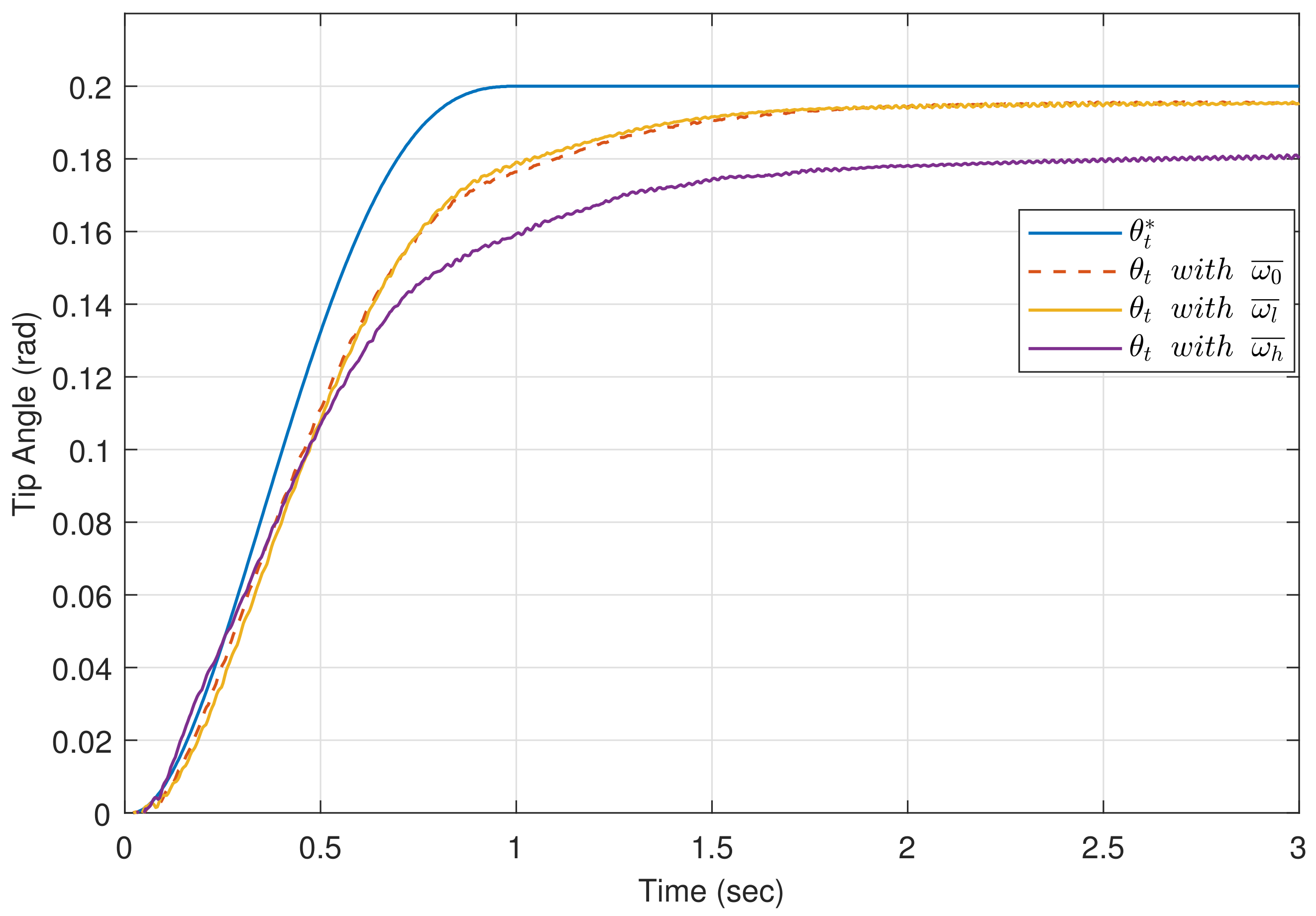
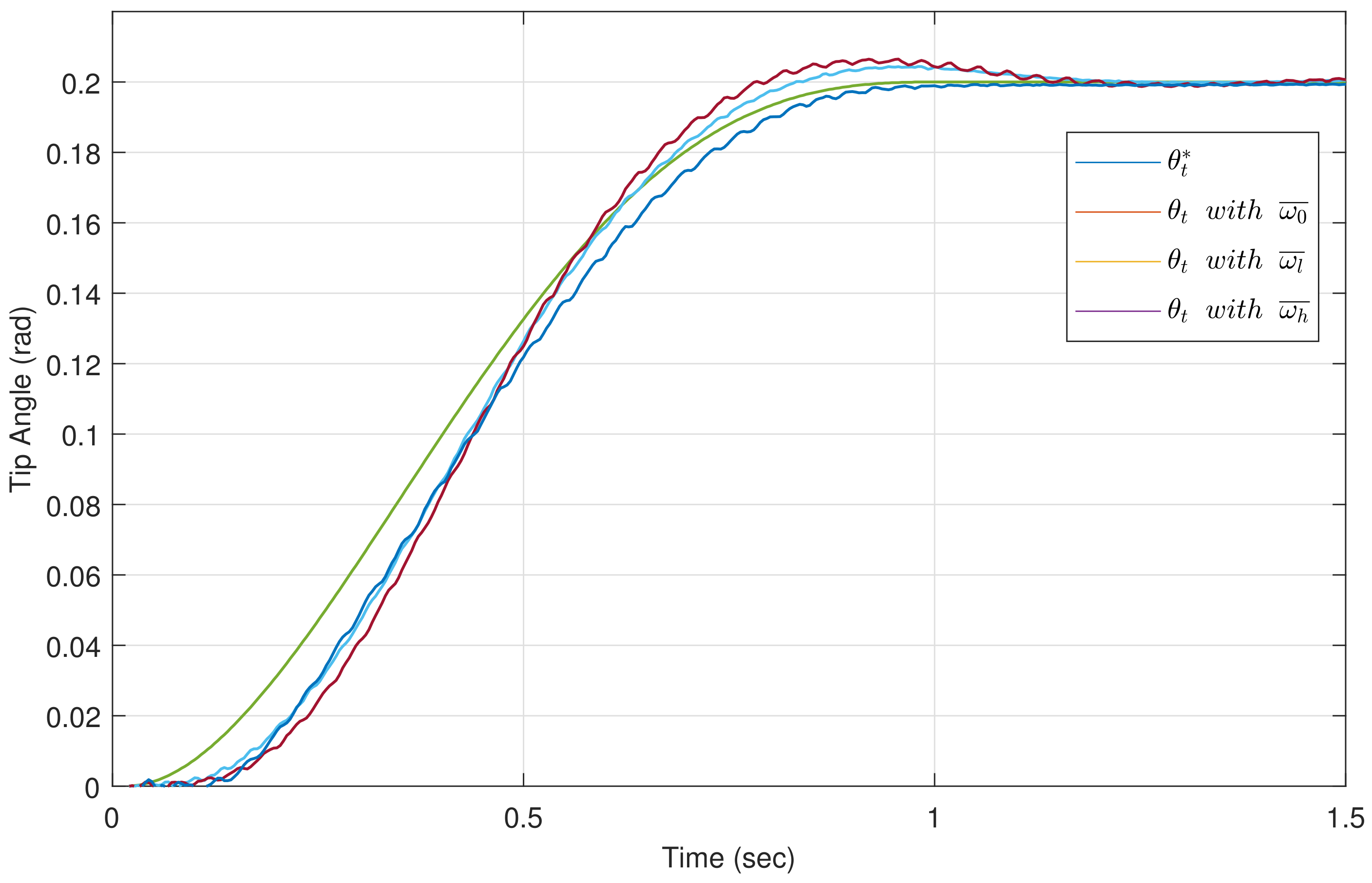
6.2. Experimental Validation of the Controller

In this subsection, the proper $FPD$ and $PD$ controllers are experimented on the setup described in Section 5. The trajectory defined in the previous subsection is used. Figure 13 shows the trajectory tracking performance of the robot using the $PD$ controller (45) in the cases of lowest, nominal and highest payloads (${\overline{\omega }}_h$, ${\overline{\omega }}_0$ and ${\overline{\omega }}_l$, respectively). The noticeable steady state error shows that this controller is unable to achieve the required tip position accuracy because it cannot remove the error caused by the offset of the strain gauge sensor. Besides, this controller shows a robust and damped response when the payload changes.

Figure 14 shows the trajectory tracking performance of the robot using the $FPD$ controller (44) in the cases of lowest, nominal and highest payloads (${\overline{\omega }}_h$, ${\overline{\omega }}_0$ and ${\overline{\omega }}_l$, respectively). The steady state error has been completely removed, which shows the ability of this controller for cancelling the effect of the offset of the strain gauge sensor. This controller shows a trajectory tracking robust to payload changes. However, the movement shows a small oscilation that is damped in the steady state. This signifies that the secondary poles introduced by the inner loop $M\left(s\right)$ in the closed-loop are less damped in the case of using the $FPD$ than in the case of using the $PD$. Figure 11 shows two very lowly damped branches (the absolute values of their imaginary components are between 27 and 63) that are the cause of this oscillation. These branches are not so close to the imaginary axes in the case of the $PD$ controller. Then the solution of this problem will be the object of a further study.

Figure 15 compares the experimental response obtained carrying the nominal disk (the same plot of Figure 14) and the simulated response using the dynamic model (3) with $\overline{\omega }=10.99$ rad/sec combined with (12) with $z=-80$. The offset of the strain gauge in this experiment, and included in the simulation is 0.0062 N·m. The error between these two responses is always lower than the $5\%$ of the total displacement of the tip (which is $0.2$ rad). This error value is small, particularly taking into account that the programmed manoeuvre is very fast (it takes about 1 sec to perform the trajectory), and fast trajectories are prone to amplify the errors between real and simulated responses, i.e., modelling errors. This result and the one shown in Figure 8 support the assumption that the before mentioned model adequately reproduces the robot dynamics.

Figure 16 shows the ability of the $FPD$ controller (44) for removing the state disturbance effects on the tip position in the case of carrying the nominal payload. The experiment consisted in hitting two times the payload at the tip. The figure shows that the tip correction is well damped and fast (it takes about $0.6$ sec returning the tip position back to its desired position). Note that the second hit is made when the transient after the first hit has not finished yet.

Finally, Figure 17 shows the control signals ${\theta }_m^{*}\left(t\right)$ generated by the outer loop in the cases of using the modified (proper) and simplified (improper) $FPD$ controllers (expressions (44) and (43), respectively). A high frequency component is observed in the case of using (43) that does not appear using (44). This illustrates the statement that the proposed proper $FPD$ reduces the high frequency noise introduced by the sensors and other sources in the control signal.

7. Conclusions

This work has developed a robust control system for a $FLR$ with a single massless link that moves in the horizontal plane. It is robust to: (1) nonlinear and time-varying motor friction, (2) offset and high-frequency noise of strain gauge sensors and (3) changes in the carried payload.

The contribution of this paper is having developed for the first time a control system robust to these three disturbances simultaneously. In order to achieve this, a two nested control loops scheme has been proposed in which the inner loop is much faster than the outer loop. This last issue allowed us to design the two control loops sequentially, implementing first a two degrees of freedom robust $PID$ controller in the inner loop and, after, applying the singular perturbation technique combined to the input-state feedback linearization method in order to design the outer loop. In the case of a second order system, this method states that the outer loop has to be closed with a $PD$ controller.

Then, our specific contribution is substituting the outer loop $PD$ by a fractional order $PD$ and developing a new tuning method based on the pole allocation technique. Our tuning method allows us to design a controller with desired time specifications for the nominal system that also achieves an isophase margin feature. This controller improves the $PD$ in two issues: it removes the sensor offset and increases the robustness to payload changes. Simulated and experimental results have been reported which illustrate these improvements. They show that a small oscillation appears during the transient in the case of the $FPD$. It is caused by the secondary branch of the root locus that appears in Figure 10. We remark that the damping of the poles of this branch can be increased by choosing poles z of the inner loop more distant from the imaginary axis (this has been verified by simulations). We could not go further than $z=-80$ in the inner loop because our computer did not allow us to use sampling times lower than 4 msec. Then this oscillation is not caused by our method but by a technological limitation.

We conclude as result of this research that:

• It is possible to remove the offset disturbance of the strain gauges of a $FLR$ without having to use controllers with an integral term—which would reduce the relative stability of the closed-loop system and the robustness to payload variations—nor differentiating the strain gauge signal, which would add noise to the closed-loop control and would compromise the compensation of some steady state tip position errors such as the errors brought about by the steady state deflections of multilink $FLR$s caused by gravity.
• The designed controller is simpler than others and provides robustness to tip payload changes larger than other controllers. For example, our controller allows payload variations from $-40\%$ to $+150\%$ of its nominal value while the robust fractional controllers [25,26] cited in the Introduction allowed only changes of $\pm 5\%$ and $\pm 25\%$, respectively, of their payload nominal values.
• Consequently, high speed motions can be achieved using a controller that can be easily designed and can be implemented in a low performance computer.
• This work prompts the design of new efficient controllers for multilink $FLR$s that will show improved robustness to torque measurement offset and payload changes. These controllers will allow fast movements with enhanced tip position precision, and will be the object of our future research.

We remark that, since our system is linear, the outer loop controller could had been designed directly using the complete dynamics of the robot with the help of a root locus such as the one of Figure 11. However, we preferred to use our procedure based on the singular perturbation technique because it has the advantage that it can be easily extended to control nonlinear systems such as multilink $FLR$, thus being the base for the development of our future controllers.

Finally, we mention that our control method, which is specially suited for $FLR$ of $1-DOF$ with one vibration mode, can be easily applied to robots with flexible joints because they also have a single vibration mode (one mode at each joint), e.g., [37].

References

- Siciliano, B.; Khatib, O. Handbook of Robotics; Springer: Berlin/Heidelberg, Germany, 2008; pp. 287–319. [Google Scholar]
- Blanc, L.; Delchambre, A.; Lambert, P. Flexible medical devices: Review of controllable stiffness solutions. Actuators 2017, 6, 23. [Google Scholar] [CrossRef] [Green Version]
- Dwivedy, S.; Eberhard, P. Dynamic analysis of flexible manipulators, a literature review. Mech. Mach. Theory 2006, 41, 749–777. [Google Scholar] [CrossRef]
- Kiang, C.T.; Spowage, A.; Yoong, C.K. Review of control and sensor system of flexible manipulator. J. Intell. Robot. Syst. 2015, 77, 187–213. [Google Scholar] [CrossRef]
- Zhou, W.; Wu, Y.; Hu, H.; Li, Y.; Wang, Y. Port-Hamiltonian modeling and IDA-PBC control of an IPMC-actuated flexible beam. Actuators 2021, 10, 236. [Google Scholar] [CrossRef]
- Ripamonti, F.; Orsini, L.; Resta, F. A nonlinear sliding surface in sliding mode control to reduce vibrations of a three-link flexible manipulator. J. Vib. Acoust. 2017, 139, 051005. [Google Scholar] [CrossRef]
- Shaheed, M.; Tokhi, O. Adaptive closed-loop control of a single-link flexible manipulator. J. Vib. Control 2013, 19, 2068–2080. [Google Scholar] [CrossRef]
- Ouyang, Y.; He, W.; Li, X. Reinforcement learning control of a single-link flexible robotic manipulator. IET Control Theory Appl. 2017, 11, 1426–1433. [Google Scholar] [CrossRef]
- Sun, C.; Gao, H.; He, W.; Yu, Y. Fuzzy neural network control of a flexible robotic manipulator using assumed mode method. IEEE Trans. Neural Netw. Learn. Syst. 2018, 29, 5214–5227. [Google Scholar] [CrossRef]
- Qiu, Z.; Zhao, Z. Vibration suppression of a pneumatic drive flexible manipulator using adaptive phase adjusting controller. J. Vib. Control 2015, 21, 2959–2980. [Google Scholar] [CrossRef]
- García-Pérez, O.; Silva-Navarro, G.P.S. Flexible-link robots with combined trajectory tracking and vibration control. Appl. Math. Model. 2019, 70, 285–298. [Google Scholar] [CrossRef]
- Dubus, G.; David, O.; Measson, Y. A vision-based method for estimating vibrations of a flexible arm using on-line sinusoidal regression. In Proceedings of the 2010 IEEE International Conference on Robotics and Automation, Anchorage, AK, USA, 3–7 May 2010; pp. 4068–4075. [Google Scholar]
- Dubus, G. On-line estimation of time varying capture delay for vision-based vibration control of flexible manipulators deployed in hostile environments. In Proceedings of the 2010 IEEE/RSJ International Conference on Intelligent Robots and Systems, Taipei, Taiwan, 18–22 October 2010; pp. 3765–3770. [Google Scholar]
- Bascetta, L.; Rocco, P. End-point vibration sensing of planar flexible manipulators through visual servoing. Mechatronics 2006, 16, 221–232. [Google Scholar] [CrossRef]
- Feliu, V.; Castillo, F.J.; Ramos, F.; Somolinos, J.A. Robust tip trajectory tracking of a very lightweight single-link flexible arm in presence of large payload changes. Mechatronics 2012, 22, 594–613. [Google Scholar] [CrossRef]
- Feliu-Talegón, D.; Feliu-Batlle, V. A Fractional-Order Controller for Single-Link Flexible Robots Robust to Sensor Disturbances; IFAC-PapersOnLine; IFAC: New York, NY, USA, 2017; Volume 50, pp. 6043–6048. [Google Scholar]
- Feliu-Talegón, D.; Feliu-Batlle, V. Control of very lightweight 2-DOF single-link flexible robots robust to strain gauge sensor disturbances: A fractional-order approach. IEEE Trans. Control Syst. Technol. 2021, 1–16. [Google Scholar] [CrossRef]
- Khalil, H.K. Nonlinear Systems; Prentice-Hall: Upper Saddle River, NJ, USA, 2002. [Google Scholar]
- Podlubny, I. Fractional Differential Equations; Academic Press: Cambridge, MA, USA, 1999. [Google Scholar]
- Dastjerdi, A.A.; Vinagre, B.M.; Chen, Y.; HosseinNia, S.H. Linear fractional order controllers; A survey in the frequency domain. Annu. Rev. Control. 2019, 47, 51–70. [Google Scholar] [CrossRef]
- Tepljakov, A.; Alagoz, B.B.; Yeroglu, C.; Gonzalez, E.; HosseinNia, S.H.; Petlenkov, E. FOPID Controllers and Their Industrial Applications: A Survey of Recent Results; IFAC-PapersOnLine; IFAC: New York, NY, USA, 2018; Volume 51, pp. 25–30. [Google Scholar]
- Oustaloup, A.; Moreau, X.; Nouillant, M. The CRONE suspension. Control. Eng. Pract. 1996, 4, 1101–1108. [Google Scholar] [CrossRef]
- Sabatier, J.; Poullain, S.; Latteux, P.; Thomas, J.; Oustaloup, A. Robust speed control of a low damped electromechanical system based on CRONE control: Application to a four mass experimental test bench. Nonlinear Dyn. 2004, 38, 383–400. [Google Scholar] [CrossRef]
- Feliu-Batlle, V. Robust isophase margin control of oscillatory systems with large uncertainties in their parameters: A fractional-order control approach. Int. J. Robust Nonlinear Control. 2017, 27, 2145–2164. [Google Scholar] [CrossRef]
- Sharma, R.; Gaur, P.; Mittal, A. Design of two-layered fractional order fuzzy logic controllers applied to robotic manipulator with variable payload. Appl. Soft Comput. 2016, 47, 565–576. [Google Scholar] [CrossRef]
- Nejad, F.; Fayazi, A.; Zadeh, H.; Marj, H.; HosseinNia, S. Precise tip-positioning control of a single-link flexible arm using a fractional-order sliding mode controller. J. Vib. Control. 2020, 26, 1683–1696. [Google Scholar] [CrossRef]
- Feliu, V.; Rattan, K.S.; Brown, H.B. Control of flexible arms with friction in the joints. IEEE Trans. Robot. Autom. 1993, 9, 467–475. [Google Scholar] [CrossRef]
- Feliu, V.; Pereira, E.; Díaz, I.M. Passivity-based control of single-link flexible manipulators using a linear strain feedback. Mech. Mach. Theory 2014, 71, 191–208. [Google Scholar] [CrossRef]
- Feliu-Talegón, D.; Feliu-Batlle, V.; Castillo-Berrio, C. Motion control of a sensing antenna with a nonlinear input shaping technique. Rev. Iberoam. Autom. Inform. Ind. 2016, 13, 162–173. [Google Scholar] [CrossRef] [Green Version]
- Ogata, K. Modern Control Engineering; Prentice-Hall: Upper Saddle River, NJ, USA, 2010. [Google Scholar]
- Shah, P.; Agashe, S. Review of fractional PID controller. Mechatronics 2016, 38, 29–41. [Google Scholar] [CrossRef]
- Monje, C.; Calderón, A.; Vinagre, B.; Feliu, V. The fractional order lead compensator. In Proceedings of the Second IEEE International Conference on Computational Cybernetics, ICCC 2004, Vienna, Austria, 30 August–1 September 2004; pp. 347–352. [Google Scholar]
- Atangana, A. On the singular perturbations for fractional differential equation. Sci. World J. 2014, 2014, 752371. [Google Scholar] [CrossRef]
- Wardi, M.L.; Amairi, M.; Abdelkrim, M.N. Fractional PID controller design for nonlinear systems based on singular perturbation technique. Int. J. Digit. Signals Smart Syst. 2018, 2, 95–120. [Google Scholar]
- Abolvafaei1, M.; Ganjefar, S. Integer-fractional decomposition and stability analysis of fractional-order nonlinear dynamic systems using homotopy singular perturbation method. Math. Control. Signals Syst. 2020, 32, 517–542. [Google Scholar] [CrossRef]
- Erickson, R.W.; Maksimovic, D. Fundamentals of Power Electronics; Kluwer Academic: New York, NY, USA, 1956. [Google Scholar]
- Cheng, X.; Liu, H.; Lu, W. Chattering-suppressed sliding mode control for flexible-joint robot manipulators. Actuators 2021, 10, 288. [Google Scholar] [CrossRef]
Publisher’s Note: MDPI stays neutral with regard to jurisdictional claims in published maps and institutional affiliations. |
© 2021 by the authors. Licensee MDPI, Basel, Switzerland. This article is an open access article distributed under the terms and conditions of the Creative Commons Attribution (CC BY) license (https://creativecommons.org/licenses/by/4.0/).
Share and Cite
Gharab, S.; Benftima, S.; Batlle, V.F. Fractional Control of a Lightweight Single Link Flexible Robot Robust to Strain Gauge Sensor Disturbances and Payload Changes. Actuators 2021, 10, 317. https://doi.org/10.3390/act10120317
Gharab S, Benftima S, Batlle VF. Fractional Control of a Lightweight Single Link Flexible Robot Robust to Strain Gauge Sensor Disturbances and Payload Changes. Actuators. 2021; 10(12):317. https://doi.org/10.3390/act10120317
Chicago/Turabian StyleGharab, Saddam, Selma Benftima, and Vicente Feliu Batlle. 2021. "Fractional Control of a Lightweight Single Link Flexible Robot Robust to Strain Gauge Sensor Disturbances and Payload Changes" Actuators 10, no. 12: 317. https://doi.org/10.3390/act10120317
APA StyleGharab, S., Benftima, S., & Batlle, V. F. (2021). Fractional Control of a Lightweight Single Link Flexible Robot Robust to Strain Gauge Sensor Disturbances and Payload Changes. Actuators, 10(12), 317. https://doi.org/10.3390/act10120317