Article

Chattering-Suppressed Sliding Mode Control for Flexible-Joint Robot Manipulators

1
College of Information Science and Technology, Donghua University, Shanghai 201620, China
2
Engineering Research Center of Digitized Textile and Apparel Technology, Ministry of Education, Shanghai 201620, China
*
Author to whom correspondence should be addressed.
Actuators 2021, 10(11), 288; https://doi.org/10.3390/act10110288
Submission received: 26 September 2021 / Revised: 17 October 2021 / Accepted: 23 October 2021 / Published: 27 October 2021
(This article belongs to the Section Actuators for Robotics)

Abstract

:
In this paper, sliding mode tracking control and its chattering suppression method are investigated for flexible-joint robot manipulators with only state measurements of joint actuators. First, within the framework of singular perturbation theory, the control objective of the system is decoupled into two typical tracking aims of a slow subsystem and a fast subsystem. Then, considering lumped uncertainties (including dynamics uncertainties and external disturbances), a composite chattering-suppressed sliding mode controller is proposed, where a smooth-saturation-function-contained reaching law with adjustable saturation factor is designed to alleviate the inherent chattering phenomenon, and a radial basis function neural network (RBFNN)-based soft computing strategy is applied to avoid the high switching gain that leads to chattering amplification. Simultaneously, an efficient extended Kalman filter (EKF) with respect to a new state variable is presented to enable the closed-loop tracking control with neither position nor velocity measurements of links. In addition, an overall analysis on the asymptotic stability of the whole control system is given. Finally, numerical examples verify the superiority of the dynamic performance of the proposed control approach, which is well qualified to suppress the chattering and can effectively eliminate the undesirable effects of the lumped uncertainties with a smaller switching gain reduced by 80% in comparison to that in the controller without RBFNN. The computational efficiency of the proposed EKF increased by about 26%.

1. Introduction

Robot manipulators with flexible joints are widely used in industrial applications due to their light weight, reduced inertia, high speed and compact structure. Joint flexibility generated from the elastic driving (by harmonic reducers, series elastic actuators or cables, etc.) always leads to vibration problem and is unavoidable in modeling, especially in applications with high-precision demands. The singularly perturbed approach has been extensively studied to model and control flexible-joint robot manipulators since it was first proven to be feasible in [1]. By such a method, the controller can be easily implemented through developing sub-controllers for the two subsystems with precisely known system dynamics, and full-state feedback [2]. Unfortunately, the actual situation is not so ideal.
It is always challenging to design controllers for robotic systems in the presence of uncertainties and/or disturbances, despite the extensive so-called robust control methods, such as robust adaptive control [3], repetitive control [4], back-stepping techniques [5], iterative learning control [6], etc. Among them, sliding mode control [7], with its simplicity in application, insensitivity to parameter variations and disturbances implicit in the input channels and non-model based robustness, remains one of the most effective approaches in handling bounded uncertainties and/or disturbances [8,9]. However, the existence of high-frequency oscillations, like chattering, restrict the application of the traditional variable structure control schemes in practical situations and have a negative impact to all chains of the feedback control loops (sensors, actuators etc.), which creates high demands on smart system integration of mechatronic applications [10,11].
For chattering suppression, refs. [12,13] designed typical sliding mode controllers (SMCs) as a second auxiliary controller that has switching gains to suppress time-delay estimation errors to achieve robust tracking performance and to weaken the negative effects of chattering. A second-order integral SMC was provided to mitigate the chattering by ensuring finite time convergence in [14,15]. As an extension, a continuous sliding mode control design was introduced in [16] to robotic systems with compliant actuators due to its advantages of strong robustness and chattering attenuation.
To a certain extent, the approaches listed above alleviate the chattering from the internal of SMC; whereas, regarding how to determinate the bounds of the unknown lumped uncertainties and avoid high switching gains that may amplify the chattering phenomenon, there are few general or effective solutions [17,18]. It was reported that the design of a controller involving a disturbance observer can balance the chattering and the switching gain. A novel integral sliding-mode-observer-based disturbance estimation scheme was designed in [17] for Euler–Lagrangian systems, and a high-order disturbance observer based sliding mode control method was designed in [18] to suppress both the mismatched and matched disturbances of system through feedforward compensation with disturbance estimation.
As an intelligent optimization mechanism, soft computing technologies include neural networks (NN), fuzzy logic, and probabilistic reasoning (evolutionary computation, chaos theory, etc.), and are preferentially considered to be integrated into the sliding mode control, to weaken the shortcomings of the classical sliding mode control strategy [19]. Such works provide some inspiration to form the proposed solution in this paper for the flexible-joint robot manipulators.
The frequently used full-state feedback controller for flexible-joint robot manipulator requires state measurements (such as angular position or velocity) from the link side, but the corresponding sensors are sometimes absent for reasons including installation difficulty or hardware cost reduction. Similar conditions also occur in the position output feedback control of rigid robot manipulators, i.e., velocity or acceleration measurements by sensors are liable to be contaminated with external noise, and are always abandoned. To handle this issue, various estimation methods in terms of observation or filtering techniques [20] are commonly incorporated to estimate the missing but required states in closed-loop control.
High-gain observers are frequently used in nonlinear feedback control, in particular in output feedback control situations [20], for the reason that they are relatively simple to design, robust to modeling uncertainty and external disturbances, and can easily achieve global or semi-global stability results. However, they are sensitive to measurement noise, and suffer from the peaking phenomenon that could even destabilize a closed-loop system if the observer gain is driven sufficiently high [21]. Sliding mode observers inherit the good robustness of the varied structure control, due to the insensitivity to uncertainties and the capability of reconstructing the uncertainties based on the equivalent injection input concept [22]. However, it is difficult to choose a filter time to suppress the high-frequency noise of the system where the undesirable chattering will degrade the estimation performance.
As a nonlinear case of Kalman filter, extended Kalman filter (EKF), is typically adopted to achieve noise rejection in the measurement process and to enhance estimation accuracy through linearizing nonlinear systems (including robotic systems) [23]. In comparison to the high-gain observer and sliding mode observer, EKF has neither peaking nor chattering phenomenon, and the ability to tolerate noise is embodied in the principle design of the EKF. However, the conventional use of EKF to observe the link states brings time-consuming computing of Jacobian matrix and worsens the implementation feasibility of EKF. Such issues are also discussed in this work.
NNs have excellent ability of nonlinear fitting and complex mapping, furthermore, their learning rules are simple and easy to implement on the digital controller [24]. Radial basis function neural network (RBFNN), as a favorable forward-feedback NN, can approximate any continuous nonlinear function with arbitrary precision, and also features rapid convergence, good adaptation and strong self-learning [25,26]; thus, it is utilized in this paper as an external factor through feedforward compensation and a class of saturation functions is applied as an internal factor in the reaching law of SMC to help suppress the chattering phenomenon caused by SMC.
To the best of our knowledge, few works have attempted to integrate the NN-based soft computing technology and sliding mode theory to design composite controllers for singularly perturbed systems. Furthermore, this is the first time in such situations to address the chattering suppression problem in SMC from a combined respective via the internal and the external of SMC. The main contributions of our work are summarized as follows.
(1)
A smooth saturation function that can obtain a sufficiently fast response characteristics near the origin to guarantee robustness through an adjustable saturation factor, is applied internally to replace the commonly used non-smooth switching function in the design of smooth-saturation-function-contained reaching law to alleviate the inherent chattering phenomenon of the sliding mode control. Simultaneously, NN-based soft computing is designed externally to run online to avoid chattering amplification caused by high value of switching gain required to cover the upper bound of the dynamics uncertainties and external disturbances. Thus, these two factors enable a chattering suppression strategy to work from both inside and outside the SMC and to help achieve superior dynamic performance of the proposed controller.
(2)
Different from the conventional treatment, by applying the concept of integral manifold within the frame of singular perturbation theory, the fast subsystem of the robot dynamics is reshaped into a typical tracking system to ensure the fast variable converges to zero over time but without considering it in the system model, thus, providing more flexibility on controller design.
(3)
An efficient EKF with a new state variable that simplifies computing the Jacobian matrix is applied to achieve closed-loop tracking control without angular position or velocity measurements of links.
(4)
Strict stability analyses on the proposed closed-loop control system in terms of two singularly perturbed subsystems and the whole system with estimation error as well as EKF are given.
In the remainder of this paper, Section 2 deals with the dynamics modeling of flexible-joint robot manipulator in framework of singular perturbation theory. In Section 3, a singularly perturbed SMC is proposed. RBFNN-based soft computing to assist the SMC with handling the dynamics uncertainties and external disturbances of the system is designed in Section 4, while Section 5 presents an EKF with new state variable to observe the states of links. Section 6 provides an overall stability analysis of the whole system, and validation examples are given in Section 7. Finally, our conclusions are given in Section 8.

2. Dynamics Model

The dynamics of an n-link flexible-joint robot manipulator can be written as [1]
M ( q ) q ¨ + C ( q , q ˙ ) q ˙ + G ( q ) + Z ( q , θ ) = 0
J θ ¨ Z ( q , θ ) = u
Z ( q , θ ) = K ( q θ )
where q , q ˙ , q ¨ R n and θ , θ ˙ , θ ¨ R n denote the angular position, velocity, and acceleration of the links and motors, respectively. M ( q ) R n × n is the positive definite inertia matrix, C ( q , q ˙ ) R n × n is the centripetal-Coriolis matrix, G ( q ) R n is the gravitational of the link dynamics, Z ( q , θ ) R n is the elastic torque at flexible joints, and K , J R n × n are positive definite constant diagonal matrices representing joint stiffness and motor inertia, respectively. u R n is the control input of motor torque. In brief, we use M , C , G and Z , to represent M ( q ) , C ( q , q ˙ ) , G ( q ) and Z ( q , θ ) , respectively, in the text that follows.
To simplify the expressions, without loss of generality, order K = k I ( I R n × n is an identity matrix), and the perturbation coefficient μ can be set as μ = 1 / k , substitute (2) and (3) into (1); then, we obtain the whole system in original singularly perturbed form with reference to the standard expression [27]
q ¨ = M 1 ( C q ˙ + G + Z )
μ Z ¨ = ( M 1 + J 1 ) Z M 1 ( C q ˙ + G ) J 1 u
To facilitate the decoupling, the concept of an integral manifold [27] is utilized to derive the slow subsystem and the fast subsystem.
We define the elastic torque Z as an integral manifold
Z = h ( q , q ˙ , θ , θ ˙ , μ , u )
where h ( q , q ˙ , θ , θ ˙ , μ , u ) (written as h for short) is assumed to be a sufficiently smooth (continuously differentiable with sufficient times) function that depends on q , θ , q ˙ , θ ˙ R n and μ .
The corresponding Taylor series expansions of h in (6) in powers of μ are given as
h = h 0 ( q , q ˙ , θ , θ ˙ , u ) + μ h 1 ( q , q ˙ , θ , θ ˙ , u ) + + μ n h n ( q , q ˙ , θ , θ ˙ , u ) +
where h i ( q , q ˙ , θ , θ ˙ , u ) is the expansion with respect to μ and can be calculated iteratively.
Let u _ s and u _ f be the control inputs for the slow subsystem and the fast subsystem, respectively, and the composite controller is given as follows:
u = u _ s + u _ f .

2.1. Slow Subsystem

Define the slow variable as h ( q , q ˙ , θ , θ ˙ , μ , u _ s ) (written as h _ s for short) in slow-scaled time t, when the joint stiffness coefficient k , i.e., μ 0 , we find q θ , h turns into h _ s , that is
h = h 0 ( q , q ˙ , θ , θ ˙ , u ) = h _ s
and u reduces to u _ s ; then, from (4) and (5), we find
q ¨ = M 1 ( C q ˙ + G + h _ s )
h _ s = ( M 1 + J 1 ) 1 [ M 1 ( C q ˙ + G ) + J 1 u _ s ]
Substituting (11) into (10), the slow subsystem can be obtained as
( M + J ) q ¨ + C q ˙ + G = u _ s
Remark 1.
The slow subsystem (12) can be recognized as the rigid part (which is essentially equivalent to the model of rigid robot manipulators) of the flexible-joint robot manipulator, and thus the existing control approaches based on the dynamics of rigid robot manipulators can be applied directly to the slow subsystem.
Remark 2.
The perturbation coefficient μ is related to the spring coefficient K . The rule for selecting μ relies on the K and the K should be sufficiently large so that the fast variables can be fast enough in fast-scaled time μ 1 t . However, in practical applications, K cannot be close to infinity, and the order of its magnitude is often 10 4 or so, i.e., the value of μ is on the order of 10 4 . Though μ is small, it is not so close to zero that a fast sub-controller for the fast subsystem is required to constrain the error caused by ignoring higher-order terms of the expansion of h in (7).

2.2. Fast Subsystem

Considering the high-order terms (which are generated by the joint flexibility and are neglected in slow subsystem) of the Taylor series expansions with respect to μ in slow subsystem in (7), we define the fast variable η as
η = Z h _ s
Recalling (5), when h turns into h _ s and u turns into u _ s , we find
μ h ¨ _ s = ( M 1 + J 1 ) h _ s M 1 ( C q ˙ + G ) J 1 u _ s
From (5), (13) and (14), we find the fast subsystem
μ η ¨ = ( M 1 + J 1 ) η J 1 u _ f
Considering (9) and (13), (15) can be rewritten as a reshaped fast subsystem
μ h ¨ 0 = ( M 1 + J 1 ) h 0 J 1 u _ f
where u _ f = u _ f J μ Z ¨ J ( M 1 + J 1 ) Z .
Remark 3.
Recalling the most commonly used expression of fast subsystem (15) proposed by Spong [1], it is necessary to calculate η and η ¨ or apply optimal control techniques [28] to work out the u _ f . In contrast, the reshaped fast subsystem (16) in this paper is actually a fast subsystem with a new control aim (different from that in [1,28,29]), to enable Z to tend to h 0 , that is to make the fast variable η converges to zero over time but without considering it in the system model, which makes the fast controller design flexible.
Therefore, it is expected in the following part to design the control laws of u _ s and u _ f for the slow subsystem (12) and the reshaped fast subsystem (16), respectively, to make q track q d (which is the desired link position) and Z track h 0 .

3. Singularly Perturbed Sliding Mode Controller

In this section, to deal with the dynamics model uncertainties and external torque disturbances for flexible-joint robot manipulators, sliding mode control strategy is adopted in the controller design for both the slow and the fast subsystems, where a class of smooth and saturation function is applied in each of the corresponding reaching law to alleviate the inherent chattering phenomenon of the sliding mode control.

3.1. Control Objective

The control objective is to design a controller that guarantees the actual link position q ( t ) R n converges asymptotically to the desired q d ( t ) R n , where we assume that, q d ( t ) is twice differentiable, q d ( t ) , and its first two derivatives are bounded for all t 0 . For any desired q d ( t ) that does not satisfy such assumption, it can be processed with the high smooth trajectory planning method proposed in [30].
In brief, the control objective can be expressed as
e ( 0 ) R n , lim t e ( t ) = 0
where the tracking error of the link position e ( t ) is defined as
e ( t ) = q d ( t ) q ( t )

3.2. Controller of Slow Subsystem

For the slow subsystem, we define a sliding surface s _ s as
s _ s = A _ s e + e ˙
where A _ s is a positive definite constant diagonal matrix, e ˙ is the derivative of e with respect to time.
Substitute (18) and (19) into (12), we find
s ˙ _ s = A _ s ( q ˙ d q ˙ ) + q ¨ d + ( M + J ) 1 ( C q ˙ + G u _ s )
As indicated in [31], the switching control law in sliding mode is not instantaneous, and the sliding surface is usually not rigorously known; this often results in a high control activity, known as chattering, which is undesirable in most systems as it can excite high-frequency dynamics that could bring the possibilities of system instability.
To reduce the chattering phenomenon from the internal of SMC, a reaching law motivated by [31] is designed as
s ˙ _ s = ϵ _ s s a t ( s _ s ) B _ s s _ s
where B _ s and ϵ _ s are positive definite constant diagonal matrices, s a t ( · ) is a monotone increasing smooth saturation function with adjustable saturation factor, passing through the origin of coordinate, continuously differentiable. More details can be found in [32]. Importantly, the smooth saturation function s a t ( · ) applied retains the fast response characteristics of the most commonly used switching function s i g n ( · ) nearby the origin to ensure sufficient robust performance, as long as the zero-crossing slope is sufficiently large. Theoretically, it can be infinitely close to the switching function s i g n ( · ) by adjusting the saturation factor but avoids discontinuous transition during switching, which is the main cause of chattering.
Through (20) and (21), the control law for the slow subsystem is presented as
u _ s = ( M + J ) [ ϵ _ s s a t ( s _ s ) + B _ s s _ s + A _ s ( q ˙ d q ˙ ) + q ¨ d ] + C q ˙ + G

3.3. Controller of Fast Subsystem

Define a sliding surface for the fast subsystem as
s _ f = A _ f η + η ˙
where A _ f is a positive definite constant diagonal matrix, η is previously defined by (13).
Substitute (23) into (16), we find
s ˙ _ f = A _ f η ˙ + Z ¨ + K [ ( M 1 + J 1 ) h 0 + J 1 u _ f ]
Similarly to (21), the reaching law for the fast subsystem controller is designed as
s ˙ _ f = ϵ _ f s a t ( s _ f ) B _ f s _ f
where B _ f and ϵ _ f are positive definite constant diagonal matrices.
Substitute (25) into (24), then the control law is derived as
u _ f = J μ [ ϵ _ f s a t ( s _ f ) + B _ f s _ f + A _ f η ˙ + Z ¨ ] J ( M 1 + J 1 ) h 0
Considering the definition of u _ f in (16), and combining with (13), (23) and (26), the control input u _ f of the fast subsystem is then obtained as
u _ f = ϵ s a t ( s _ f ) + K p η + K d η ˙
where ϵ = J μ ϵ _ f , K p = J μ B _ f A _ f J ( M 1 + J 1 ) , K d = J μ ( A _ f + B _ f ) .
Remark 4.
Formula (27) can be recognized as a proportional-derivative (PD) control law relating to the error term η , with a sliding mode term ϵ s a t ( s _ f ) , then the performance of the fast system can be optimized by the parameters tuning rules for PD controllers. It is not necessary to involve Z ¨ or η ¨ as [1], which improves the computation efficiency and engineering practicality. The sliding mode term increases the robustness of the boundary layer and makes the fast subsystem more stable.
Remark 5.
The control aim of the fast subsystem is to enable the elastic torque of the joint Z to track the h 0 , which can be taken as further fine tuning to the torque control input of the slow subsystem u _ s . Note that, although according to (27), K p is a time-varying gain that varies as the inertia matrix M changes, M is bounded by property 1 in [20] and the corresponding bounded value of K p is not so sensitive to the control performance. Hence, K p can be selected properly as a constant diagonal matrix to simplify the control law.

4. RBFNN-Based Soft Computing Strategy

Considering the uncertainties of the dynamics model and disturbances of the torque control input, the expressions (12) and (15) for flexible-joint robot manipulators can be rewritten as
( M + J ) q ¨ + C q ˙ + G + Δ ( M + J ) q ¨ + Δ C q ˙ + Δ G = u _ s + d 1
μ η ¨ = ( M 1 + J 1 ) η J 1 u _ f Δ ( M 1 + J 1 ) η Δ J 1 u _ f + d 2
where Δ ( M + J ) , Δ C , Δ G , Δ ( M 1 + J 1 ) and Δ J 1 denote the uncertainties of each term of the model, d 1 and d 2 are the disturbance terms of the control inputs to slow subsystem and fast subsystem, respectively.
From (28) and (29), we find
q ¨ = ( M + J ) 1 ( u _ s C q ˙ G ) δ _ s
η ¨ = K [ ( M 1 + J 1 ) η J 1 u _ f ] + δ _ f
where δ _ s = ( M + J ) 1 [ Δ ( M + J ) q ¨ + Δ C q ˙ + Δ G d 1 ] , and δ _ f = K [ Δ ( M 1 + J 1 ) η + Δ J 1 u _ f d 2 ] are the uncertainties and disturbances of the slow subsystem and the fast subsystem, respectively.
Remark 6.
The robustness of sliding mode is closely related to its switching gain. When the model parameters are uncertain due to inaccuracy of parameter identification, and the switching gain needs to be adjusted in response. The gains (especially ϵ _ s ) of the proposed SMC should be adjusted to be large enough to cover the bounds (which are susceptible to changes in model parameters) of the system uncertainties and external disturbances (in (30) and (31)) and to reject the resulted undesirable effects. Although the chattering phenomenon is reduced greatly by the reaching law involving smooth saturation function, such high coefficients in the switching control (by (21) and (25)) will still enlarge the influence of chattering. Meanwhile, the bounds of the system uncertainties and/or external disturbances are always unknown and difficult to determine. Hence, RBFNN-based soft computing strategy is applied subsequently to provide feedforward compensation to alleviate the pressure of SMC to process lumped uncertainties and to help enhance the overall performance of SMC, which will be verified in Section 7.
RBF-based soft computing is designed for each subsystem individually, and is running online. According to [25], we define the input layer of the RBFNN as error term E = [ E 1 T , E 2 T , , E n T ] T , where E i ( i = 1 , 2 , , n ) is the error vector of either the slow subsystem E i _ s or the fast subsystem E i _ f of the i-th joint:
E i = E i _ s = [ e i e i ˙ ] T , for slow subsystem E i _ f = [ η i η i ˙ ] T , for fast subsystem
and the hidden layer as the radial basis function Φ = [ ϕ 1 T , ϕ 2 T , , ϕ n T ] T , where ϕ i ( i = 1 , 2 , , n ) is the radial basis function (Gaussian kernal) of either the slow subsystem ϕ i _ s or the fast subsystem ϕ i _ f of the i-th joint, the j-th activation function ϕ i j ( ϕ i j _ s or ϕ i j _ f ) of ϕ i ( ϕ i _ s or ϕ i _ s ) is given as
ϕ i j = exp ( | | E i T i j | | 2 2 U i 2 )
where j = 1 , 2 , , m , m is the node number of the hidden layer. T i and U i are the center matrix and base width of the i-th joint, respectively. T i j is the center vector corresponding to the j-th weight value of the i-th joint.
Suppose the fitting error is small enough, and the i-th joint error δ i ( δ i _ s or δ i _ f ) of the (slow or fast) subsystem can be expanded into δ i = W i T ϕ i , where W i ( W i _ s or W i _ f ) is the ideal connecting weight value between the hidden layer and the output layer. Thus, the actual i-th joint output layer δ ^ i of the NN can be designed as
δ ^ i = W ^ i T ϕ i
where W ^ i ( W ^ i _ s or W ^ i _ f ) is the approximate value of the ideal connecting weight matrix W i .
The adaptive control law is designed as
W ^ ˙ i = γ i s i ϕ i
where γ i ( γ i _ s or γ i _ f ) is a constant and s i ( s i _ s or s i _ f ) is the sliding surface of the i-th joint.
Remark 7.
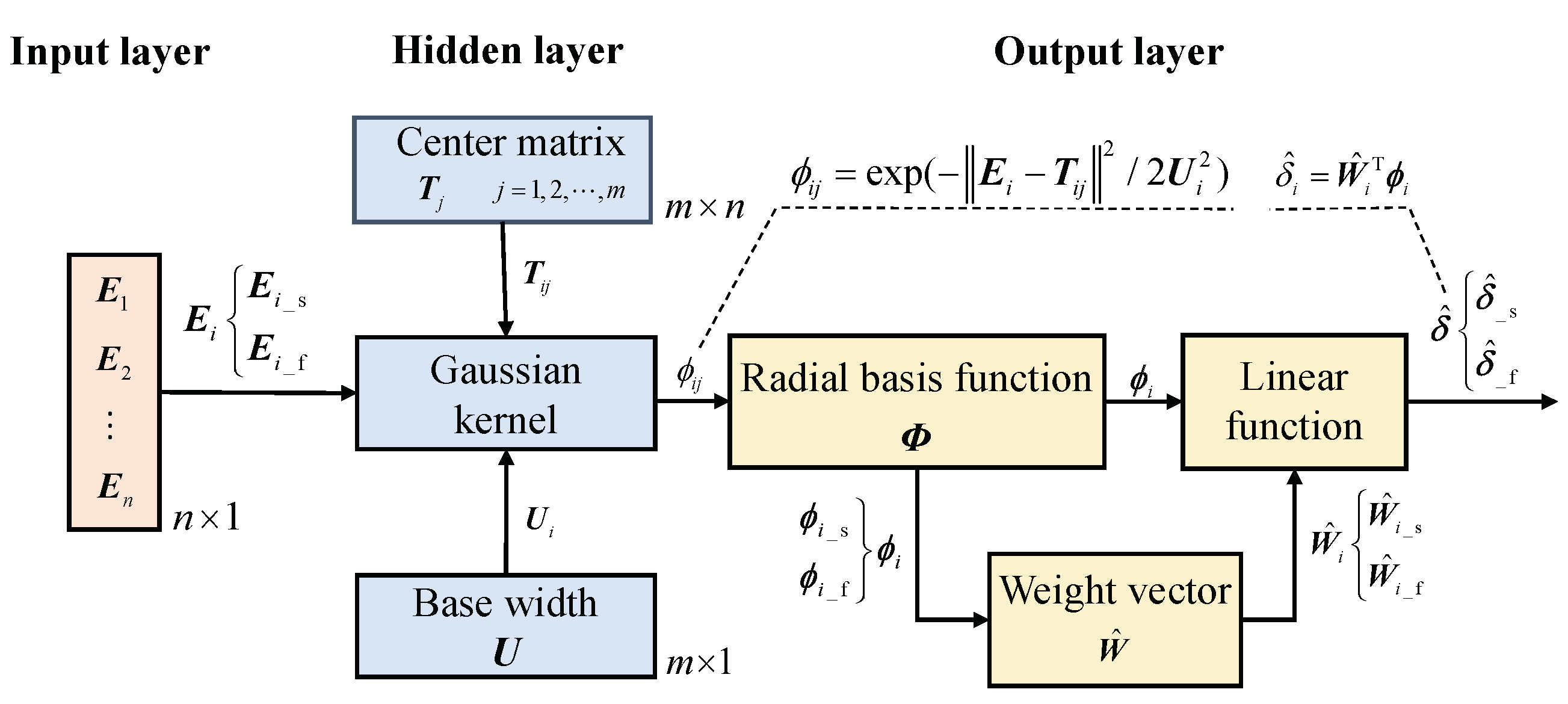
Unlike the traditional NNs [33,34,35] that have to rely on time-consuming off-line training to optimize the model, the RBFNN-based compensator designed in this paper is in online self-adjusting working mode with simple structure and small computing burden. It is a three-layer forward network. The mapping from input to output is nonlinear, while the mapping from hidden layer to output layer is linear. Importantly, the RBFNN is a local approximation NN that can greatly speed up the learning and is suitable for real-time control requirements. Its operational structure is sketched by Figure 1, where the E i ( i = 1 , 2 , , n ) in the input layer is the error term defined by (32), the Gaussian kernel by (33) is chosen in the hidden layer for the RBF, and the δ ^ i in the output layer is the approximation of the error of i-th joint caused by dynamics model uncertainties and joint torque disturbances and is updated by (34) with the adaptive control law (35).
Finally, the control law (22) and (27) can be rewritten as
u _ s = ( M + J ) [ ϵ _ s s a t ( s _ s ) + B _ s s _ s + A _ s ( q ˙ d q ˙ ) + q ¨ d ] + C q ˙ + G + ( M + J ) δ ^ _ s
u _ f = ϵ s a t ( s _ f ) + K p η + K d η ˙ + J μ δ ^ _ f
where δ ^ _ s = [ δ ^ 1 _ s , δ ^ 2 _ s , , δ ^ n _ s ] T is the output layer of the RBFNN for the slow subsystem, and ( M + J ) δ ^ _ s is the compensation term of its control input, while for the fast subsystem, δ ^ _ f = [ δ ^ 1 _ f , δ ^ 2 _ f , , δ ^ n _ f ] T is the output layer of its RBFNN and J μ δ ^ _ f is the compensation term of its control input.
Remark 8.
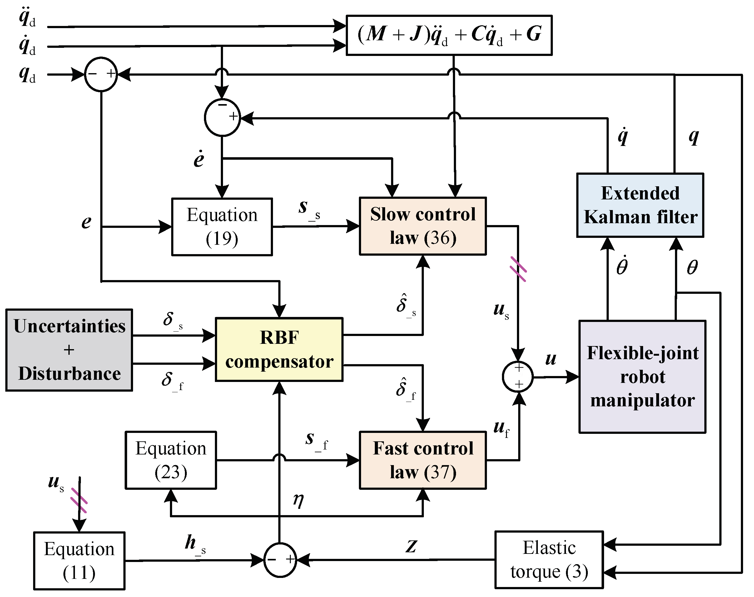
As presented by (8), (36), and (37), inheriting the idea of decomposing the whole dynamics of an n-degree-of-freedom flexible-joint robot manipulator by (1) and (2) into two subsystems in the framework of singular perturbation theory, u _ s acts on the slow subsystem (rigid part), while u _ f acts on the fast subsystem (flexible part) to depress the influence caused by the joint flexibility. Both sub-controllers are designed with the sliding mode control strategy, where the q and q ˙ involved are obtained from the EKF proposed in Section 5, making the closed-loop control without measuring link states. Moreover, an RBFNN-based error compensator is included in the proposed SMC. The block diagram of the proposed control approach is shown in Figure 2.

5. Extended Kalman Filter

Considering the control law presented by (36) and (37), at least four feedback variables q , q ˙ , θ and θ ˙ are required to accomplish the closed-loop tracking control. Actually, the corresponding sensors to measure the states of the links are usually missing. In this section, an efficient EKF based on a new state variable is proposed to estimate the position and velocity of the links.

5.1. EKF with Conventional State Variable

First, let us recall the design process of an EKF based on a conventional state variable, in terms of flexible-joint robot manipulator [23].
The most commonly used state variable x is defined as
x = [ q T q ˙ T θ T θ ˙ T ] T = [ x 1 T x 2 T x 3 T x 4 T ] T
The time derivative function f ( x ) of the state variable x is obtained as
f ( x ) = x ˙ = q ˙ M 1 [ C q ˙ + G + K ( q θ ) ] θ ˙ J 1 [ u + K ( q θ ) ]
and the partial derivative of the state function with respect to the states can be written as:
f ( x ) x = F ( t ) = 0 I 0 0 F 1 F 2 F 3 0 0 0 0 I F 4 0 F 5 0
where
F 1 = M 1 [ M q q ¨ + C q q ˙ + G q + K ] , F 2 = M 1 ( C q ˙ + C ) , F 3 = M 1 K , F 4 = F 5 = J 1 K .
Define observation vector as h ( x ) = [ θ T θ ˙ T ] T = [ x 3 T x 4 T ] T , the partial differential equation of the observation vector with respect to the states is
h ( x ) x = H ( t ) = 0 0 I 0 0 0 0 I
Considering (39)–(41), the EKF based on a conventional state variable defined by (38) is expressed as
x ^ ˙ = f ( x ^ , u ) + L ( t ) [ y ( t ) h ( x ^ ) ]
P ˙ ( t ) = F ( t ) P ( t ) + P ( t ) F T ( t ) + Q ( t ) L ( t ) H ( t ) P ( t )
L ( t ) = P ( t ) H T ( t ) R 1 ( t )
where x ^ is the estimation of x , u is defined by (8), y ( t ) = h ( x ) is the output, L ( t ) is a time-varying matrix and denotes the Kalman filtering gain, P ( t ) is a positive definite symmetric matrix and denotes the covariance under state x , Q ( t ) and R ( t ) are positive definite symmetric matrices and denote the covariances of the process noise and observation noise, respectively.

5.2. EKF with New State Variable

As presented, it is complicate to calculate the Jacobian matrix F ( t ) expressed by (40), where large amounts of time-consuming calculations of partial derivatives with respect to q and q ˙ are needed.
To simplify the EKF algorithm, a new state variable definition is given in this paper as
x = [ Z T Z ˙ T θ T θ ˙ T ] T = [ x 1 T x 2 T x 3 T x 4 T ] T
where q and q ˙ are implicitly contained in Z and Z ˙ , respectively.
Now, the time derivative function f ( x ) of the state variable x can be expressed as
f ( x ) = x ˙ = Z ˙ K [ ( M 1 + J 1 ) Z + M 1 ( C q ˙ + G ) + J 1 u ] θ ˙ J 1 ( u + Z )
and the partial derivative of the state function with respect to the new states is obtained as
f ( x ) x = F ( t ) = 0 I 0 0 K ( M 1 + J 1 ) 0 0 0 0 0 0 I J 1 0 0 0
After Z and Z ˙ are observed by the proposed EKF with new state variable, we finally find the estimations of q and q ˙ through (3), respectively.
Remark 9.
It can be found that, in the EKF with conventional state variable [23], q and q ˙ are involved explicitly in the state variable x , which results in complicated calculations of the corresponding partial derivatives, as well as computing M ˙ 1 , C ˙ and G ˙ . While in the proposed EKF with new state variable, instead of q and q ˙ , Z and Z ˙ are adopted as the states, then the corresponding partial derivatives of M 1 , C and G are all zero, which improves the computing efficiency greatly.

6. Stability Analysis

The overall stability of the closed-loop system in terms of two singularly perturbed subsystems and also whole system with the proposed EKF and RBFNN-based soft computing involved sliding mode control approach is analyzed by the following steps.
Step 1: The stability analysis of the slow subsystem.
Theorem 1.
Consider the dynamics of the slow subsystem described by (30) with the proposed sub-controller (36), it results in asymptotic convergence of the state and output tracking errors in the sense that | | e | | , | | e ˙ | | 0 , as t .
Proof. 
Considering the approximation error of the connecting weight value caused by RBF based soft computing in slow subsystem, a Lyapunov function candidate V 1 is defined as
V 1 = 1 2 s _ s T s _ s + i = 1 n 1 2 γ i _ s W ˜ i _ s T W ˜ i _ s
where the approximation error of connecting weight in slow subsystem is defined as W ˜ i _ s = W ^ i _ s W i _ s . Clearly, V 1 is positive definite.
Take the derivative of V 1 with respect to time t, and substitute (30) and (36) into it, we find
V ˙ 1 = s _ s T [ ϵ _ s s a t ( s _ s ) + B _ s s _ s ] + i = 1 n W ˜ i _ s T ( 1 γ i _ s W ^ ˙ i _ s s i _ s ϕ i _ s )
Substitute (35) into (49)
V ˙ 1 = s _ s T [ ϵ _ s s a t ( s _ s ) + B _ s s _ s ]
By recalling the definitions of sliding surface (19) and the reaching law (21) for slow subsystems, as well as the monotonicity of saturation function s a t ( · ) , we find that V ˙ 1 is negative definite, and the slow subsystem is asymptotic stable in the sense that | | e | | , | | e ˙ | | 0 as t , due to the positive definiteness of V 1 and the negative definiteness of V ˙ 1 . □
Step 2: The stability analysis of the fast subsystem.
Theorem 2.
Consider the dynamics of the fast subsystem described by (31) with the proposed sub-controller (37): if
2 λ m i n ( B _ f ) λ m i n ( A _ f ) 1 4 σ m a x 2 ( A _ f ) > 0
is satisfied, where λ m i n ( · ) and σ m a x ( · ) are the minimum eigenvalue and the maximum singular value of matrix, respectively, then it results in asymptotic convergence of the state and output tracking errors in the sense that | | η | | , | | η ˙ | | 0 , as t .
Proof. 
Considering the approximation error of the connecting weight value caused by RBF based soft computing in fast subsystem, a Lyapunov function candidate V 2 is defined as
V 2 = μ 1 [ s _ f T s _ f + i = 1 n 1 γ i _ f W ˜ i _ f T W ˜ i _ f + 1 2 ( A _ f η ) T ( A _ f η ) ]
where the approximation error of connecting weight in fast subsystem is defined W ˜ i _ f = W ^ i _ f W i _ f . Clearly, V 2 is positive definite.
Substitute (23) and (31) into (52), then take the derivative of V 2 with respect to the fast-scaled time μ 1 t , we find -4.6cm0cm
V ˙ 2 = 2 s _ f T { A _ f η ˙ K [ ( M 1 + J 1 ) η + J 1 u _ f ] + δ _ f } + i = 1 n 2 γ i _ f W ˜ i _ f T W i _ f ^ ˙ + s _ f T A _ f η ˙ η ˙ T A _ f η ˙
Substitute (37) and (35) into (53) in sequence, and we have
V ˙ 2 2 s _ f T ϵ _ f s a t ( s _ f ) [ s _ f T η ˙ T ] D 1 [ s _ f T η ˙ T ] T
where
D 1 = 2 λ m i n ( B _ f ) 1 2 σ m a x ( A _ f ) 1 2 σ m a x ( A _ f ) λ m i n ( A _ f ) .
To ensure V ˙ 2 is negative definite, together with considering the monotonicity of saturation function s a t ( · ) , D 1 should be positive definite, i.e., inequality (51) is to be satisfied by proper selection of positive definite constant diagonal matrices A _ f and B _ f . Thus the asymptotic stability of the fast subsystem is achieved if constraint condition (51) is satisfied. □
Step 3: The stability analysis of the whole system.
Note that, the slow subsystem (30) involved in Step 1 is an approximate model based on (12), which is derived by assuming the joint stiffness coefficient k , it is not qualified to present the complete dynamics by (10). Thus, in the stability analysis of the whole system, we need an updated expression of (30) from (10) with considering uncertainties of dynamics model and disturbance of the torque control input:
q ¯ ¨ = M 1 ( h _ s + η + C q ˙ + G ) + δ ¯ _ s
where δ ¯ _ s = M 1 ( Δ M q ¨ + Δ C q ˙ + Δ G d 1 ) .
Substitute (11) and (36) into (55), we find
q ¯ ¨ = ϵ _ s s a t ( s _ s ) + B _ s s _ s + A _ s ( q ˙ d q ˙ ) + q ¨ d + δ ^ _ s M 1 η + δ ¯ _ s
Theorem 3.
Consider the dynamics of the whole system described by (55) and (31) with the proposed sub-controller (8), (36) and (37), if the following inequalities
λ m i n ( B _ s ) λ m i n ( B _ f ) λ m i n 2 ( A _ f ) σ m a x 2 ( M 1 ) > 0
λ m i n 2 ( B _ f ) 1 4 σ m a x 2 ( A _ f ) > 0
3 4 λ m i n ( B _ f ) λ m i n 3 ( A _ f ) σ m a x 2 ( B _ f ) σ m a x 2 ( A _ f ) > 0
are satisfied, then it results in asymptotic convergence of the whole system and the control objective (17) is achieved.
Proof. 
Consider a Lyapunov function candidate V as
V = a V 1 + b V 2
where a and b are both positive constant. Similar to [29], we also select a = b = 1 . It is easy to find that V is positive definite.
Substitute (56), (23), (31), (37) into V ˙ in sequence, we have
V ˙ = V ˙ 1 + V ˙ 2 s _ s T ϵ s a t ( s _ s ) 2 s _ f T ϵ s a t ( s _ f ) [ s _ s T η T ] D 2 [ s _ s T η T ] T [ s _ f T η ˙ T ] D 3 [ s _ f T η ˙ T ] T [ η T η ˙ T ] D 4 [ η T η ˙ T ] T
where
D 2 = λ m i n ( B _ s ) 1 2 σ m a x ( M 1 ) 1 2 σ m a x ( M 1 ) 1 4 λ m i n ( B _ f ) λ m i n 2 ( A _ f ) , D 3 = λ m i n ( B _ f ) 1 2 σ m a x ( A _ f ) 1 2 σ m a x ( A _ f ) λ m i n ( B _ f ) , D 4 = 3 4 λ m i n ( B _ f ) λ m i n 2 ( A _ f ) σ m a x ( B _ f ) σ m a x ( A _ f ) σ m a x ( B _ f ) σ m a x ( A _ f ) λ m i n ( A _ f ) .
It can be found that, V ˙ will be negative definite if D 2 , D 3 and D 4 are all positive definite, i.e., the inequalities (57)–(59) are to be satisfied by proper selection of positive definite constant diagonal matrices A _ f , B _ s and B _ f .
Thus, the whole system yields asymptotic stability through the positive definitiveness of V and the negative definitiveness of V ˙ , and the control goal (17) is achieved. □
Step 4: The stability analysis of the EKF with new state variable.
For the proposed EKF, we first expand f ( x ) and h ( x ) by
f ( x ) f ( x ^ ) = F ( t ) ( x x ^ ) + φ
h ( x ) h ( x ^ ) = H ( t ) ( x x ^ ) + χ
where φ and χ are the terms of the second and higher orders in ( x x ^ ).
We define the observation error as
ζ = x x ^
and then, from (39), (42), (62) and (63), we find
ζ ˙ = [ F ( t ) L ( t ) H ( t ) ] ζ + φ L ( t ) χ
The proof of exponential stability of the proposed EKF is equivalent to certifying that the differential Equation (65) for the observation error is exponentially stable at 0 [36]. To facilitate the expressions, F , H , L , P and Q are used to represent F ( t ) , H ( t ) , L ( t ) , P ( t ) and Q ( t ) , respectively.
Theorem 4.
Consider the nonlinear system of flexible-joint robot manipulator by (55), (31) and the proposed EKF by (42)–(45), without loss of generality, let the following assumptions: | φ | | k φ | | ζ | | 2 , | | χ | | k χ | | ζ | | 2 , | | H | | h ¯ , p ̲ I P p ¯ I , q ̲ I Q and r ̲ I R hold, where k φ , k χ , h ¯ , p ̲ , p ¯ , q ̲ and r ̲ are all positive constants, I is the identity matrix with the same dimensions as P , Q and R , then there are positive constants ε, α and β such that the proposed EKF is exponentially stable, i.e.,
| | ζ ( t ) | | α | | ζ ( 0 ) | | e β t
holds for every t 0 and for every solution ζ ( · ) of (65) with ζ ( 0 ) B ε ( B ε = υ R 4 n : | | υ | | ε ) .
Proof. 
Define Y as
Y = P 1 ( t )
Consider a Lyapunov function candidate as
V 3 = ζ T Y ζ
where Y is positive definite due to that P ( t ) is positive definite; therefore, the positive definiteness of V 3 is guaranteed.
After taking the time derivative of V 3 , considering P T = P , Y ˙ = Y P ˙ Y , (43), (44) and (65), we obtain
V ˙ 3 = ζ T [ Y Q Y + H T ( R 1 ) T H ] ζ + ( φ L χ ) T Y ζ + ζ T Y ( φ L χ )
Note that the term H T ( R 1 ) T H in (69) is positive definite, then we have
V ˙ 3 [ q ̲ p ¯ 2 + ( 2 k φ p ̲ + 2 h ¯ k χ r ̲ ) | | ζ | | ] | | ζ | | 2
Hence, for all | | ζ | | ε with ε = m i n ( ε , r ̲ p ̲ q ̲ 4 p ¯ 2 ( r ̲ k φ + p ̲ h ¯ k χ ) ) , where ε is defined in (66), we have
V ˙ 3 ( t ) q ̲ 2 p ¯ 2 | | ζ ( t ) | | 2 q ̲ p ̲ 2 p ¯ 2 V 3 ( t )
and the solution of (71) is
V 3 ( t ) V 3 ( 0 ) e q ̲ p ̲ 2 p ¯ 2 t
From (68) and (72), it leads to
| | ζ ( t ) | | p ¯ p ̲ | | ζ ( 0 ) | | e q ̲ p ̲ 4 p ¯ 2 t ,
i.e., the inequality (66) is achieved with α = p ¯ p ̲ and β = q ̲ p ̲ 4 p ¯ 2 , and thus the exponential stability of the EKF with new state variable is guaranteed. □
Finally, the asymptotic stability of the whole system with the proposed EKF is achieved if (51), (57)–(59), and the assumptions in Theorem 4 hold.

7. Validation Example

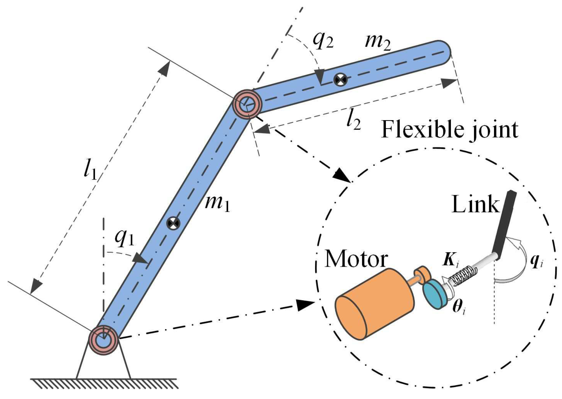
The proposed scheme is verified on a two-link flexible-joint robot manipulator shown in Figure 3. Its parameters are given as
M = 9.77 + 2.02 cos q 2 1.26 + 1.01 cos q 2 1.26 + 1.01 cos q 2 1.12 , C = 1.01 q ˙ 2 sin q 2 1.01 ( q ˙ 2 + q ˙ 1 ) sin q 2 1.01 q ˙ 1 sin q 2 0 , G = 79.38 sin q 1 + 11.074 sin ( q 1 + q 2 ) 11.074 sin ( q 2 + q 1 ) , K = d i a g ( 10000 , 10000 ) , J = d i a g ( 0.1 , 0.1 ) ,
and the model uncertainties Δ M , Δ C and Δ G set as 20% of M , C and G , respectively, as well as the joint torque disturbances d 1 and d 2 set as d i a g ( 15 , 15 ) N · m to the slow subsystem and d i a g ( 5 , 5 ) N · m to the fast subsystem during 5.5 s to 6.5 s.
Considering the stability constraints of the control system by (30) and (31), the parameters in the proposed control scheme are finally set as A _ s = d i a g ( 7 , 7 ) , B _ s = d i a g ( 10 , 10 ) , ϵ _ s = d i a g ( 10 , 10 ) , A _ f = d i a g ( 400 , 400 ) , B _ f = d i a g ( 250 , 250 ) , K p = d i a g ( 1 , 1 ) , K d = d i a g ( 0.065 , 0.065 ) , ϵ = d i a g ( 0.0001 , 0.0001 ) , γ 1 _ s = γ 2 _ s =2000, γ 1 _ f = γ 2 _ f = 1 , T 1 _ s = T 2 _ s = T 1 _ f = T 2 _ f = [ 1 , 0.5 , 0 , 0.5 , 1 ; 1 , 0.5 , 0 , 0.5 , 1 ] , U 1 _ s = U 2 _ s = U 1 _ f = U 2 _ f = 3 , and the saturation function s a t ( · ) is selected to be arc tangent a t a n ( · ) . The desired trajectories of two links are given by
q l d = 1 5 π sin ( 5 π t + π 6 ) sin ( 5 π t + π 7 ) ( rad )

7.1. Verification of the Proposed Sliding Mode Control Strategy

To verify the proposed scheme in presence of dynamics uncertainties and joint torque disturbances under full-state feedback, comparisons between the proposed controller without EKF (named as SMC+RBF) and the proposed controller without EKF or RBF (named as SMC) are made, where two additional sets, i.e., d i a g ( 40 , 40 ) and d i a g ( 50 , 50 ) of ϵ _ s are added for controller SMC.
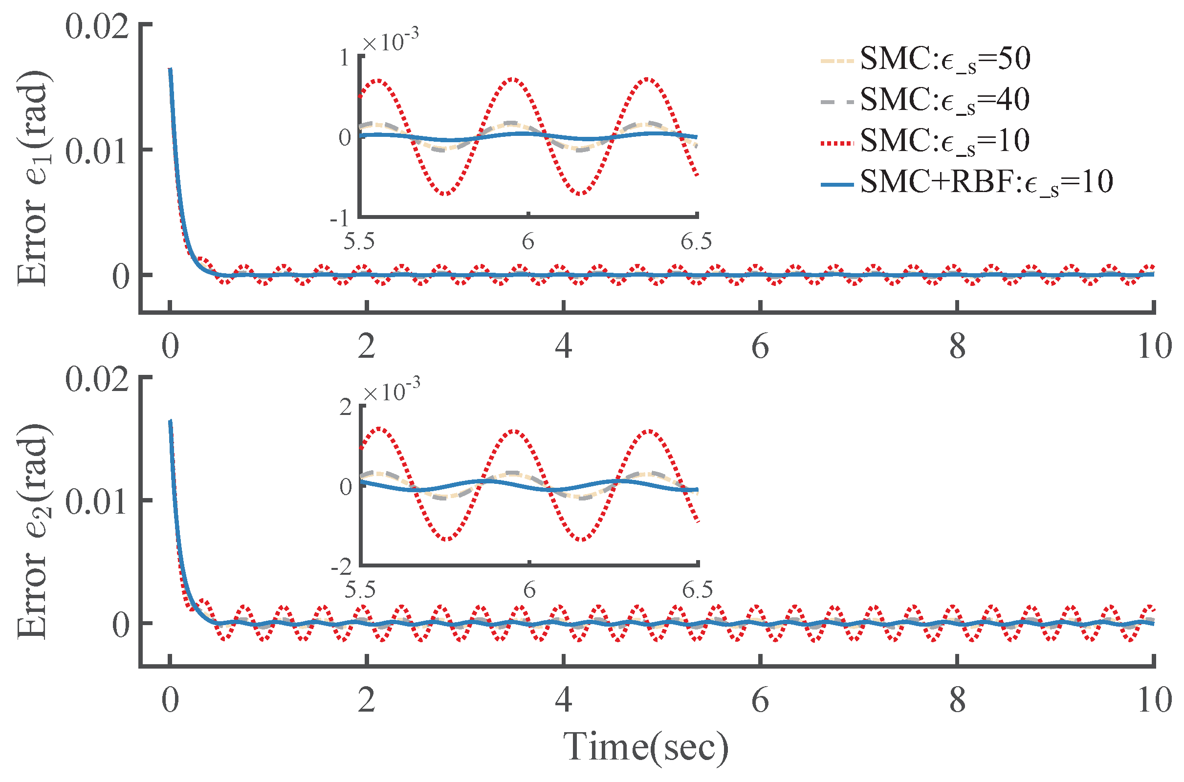
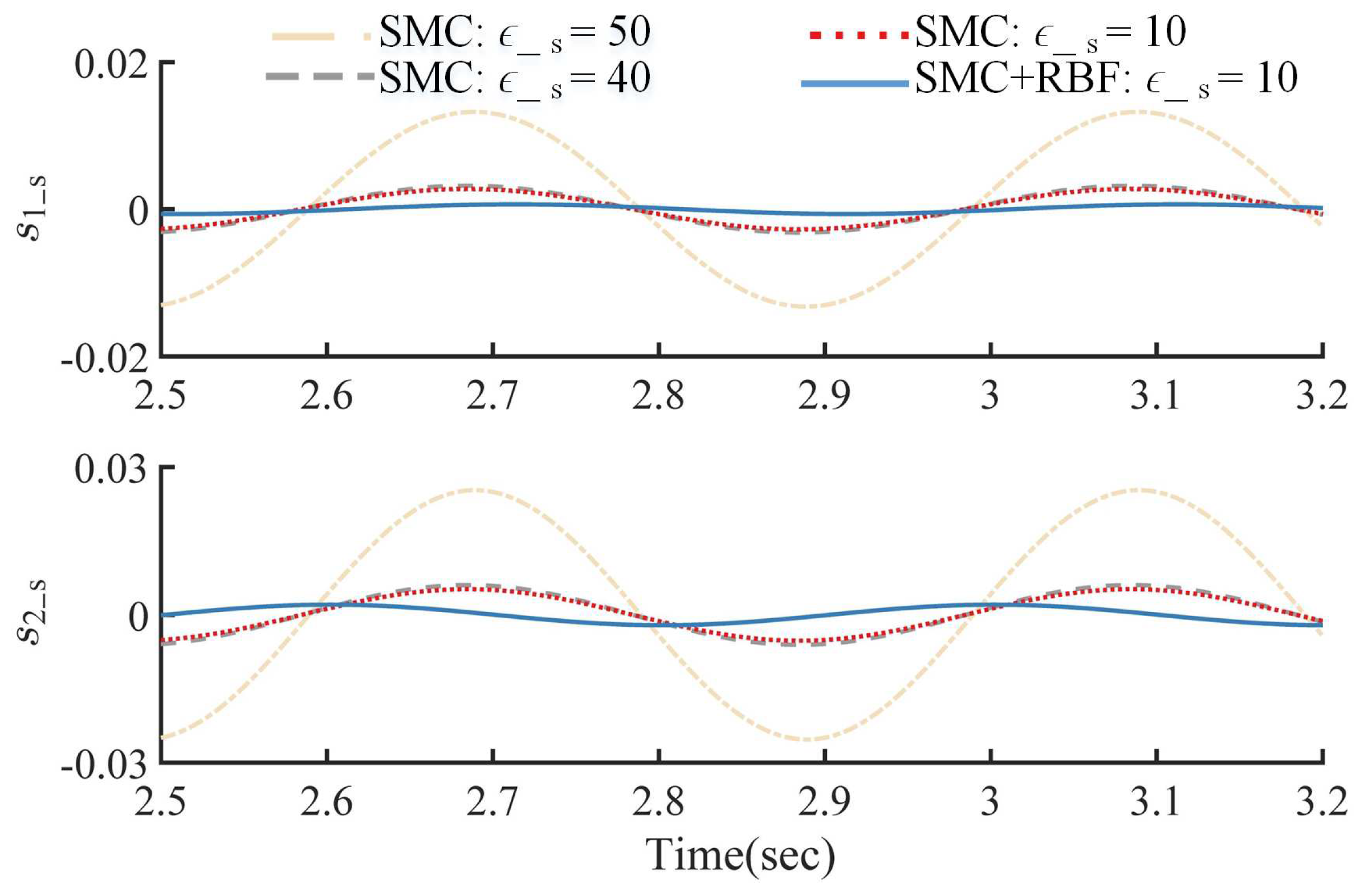
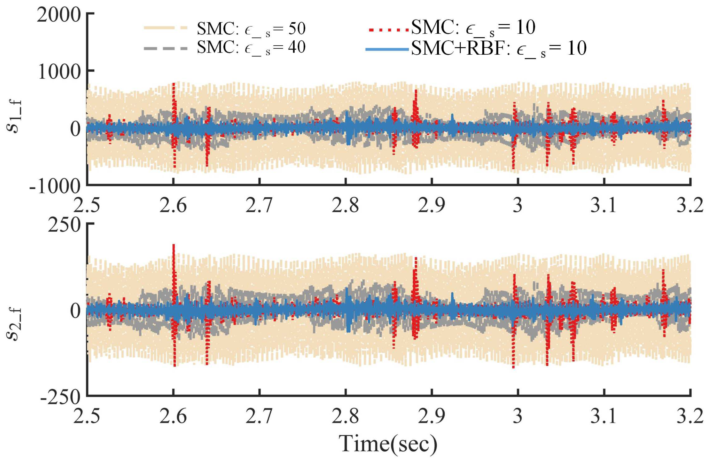
As shown in Figure 4, Figure 5, Figure 6 and Figure 7, in controller SMC, when ϵ _ s becomes larger, the influence of uncertainty and disturbance on the system is smaller and the trajectory tracking accuracy of the SMC becomes higher. However, the chattering phenomenon previously suppressed by the proposed switching control becomes worse. Especially when the parameter is changed from 40 to 50, the trajectory tracking effect is not significantly improved, but the chattering phenomenon is extremely deteriorated.
With RBFNN-based soft computing to avoid such problem, the controller SMC+RBF shows superior tracking performance with smaller value of ϵ _ s (which is reduced by 80%). It is worth mentioning that the RBF-based soft computing can assist the proposed SMC to better eliminate adverse effects caused by lumped uncertainties and achieve better control performance through generating torque compensation of feedforward type as shown in Figure 7, without increasing the value of ϵ _ s or determining the bounds of the system uncertainties and external disturbances.

7.2. Verification of the Proposed EKF

To test the proposed EKF, comparisons to the EKF with conventional state variable [23] were made, where the process noise and observation noise to every state variable of each link were assumed to be independent and constant, i.e., Q = I , R = I , where I is the identity matrix. The initial P is set as P ( 0 ) = I . In addition, the random noise within amplitude of 0.001 rad is assumed to be mixed in the position observations of each link by the proposed EKF with new state variables. The trajectories of two links to be observed are given as
q d = 1 10 π sin ( 10 π t ) sin ( 10 π t ) ( rad )
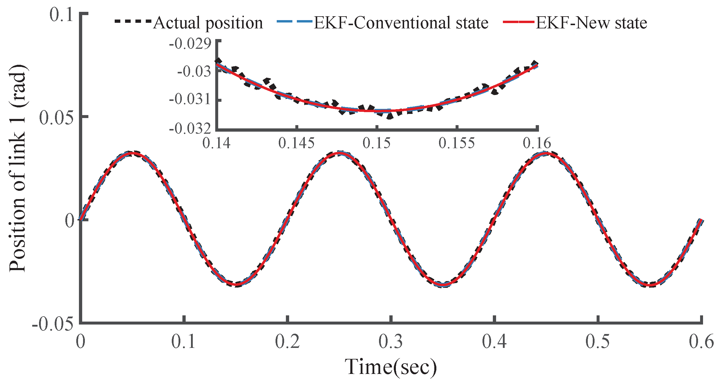
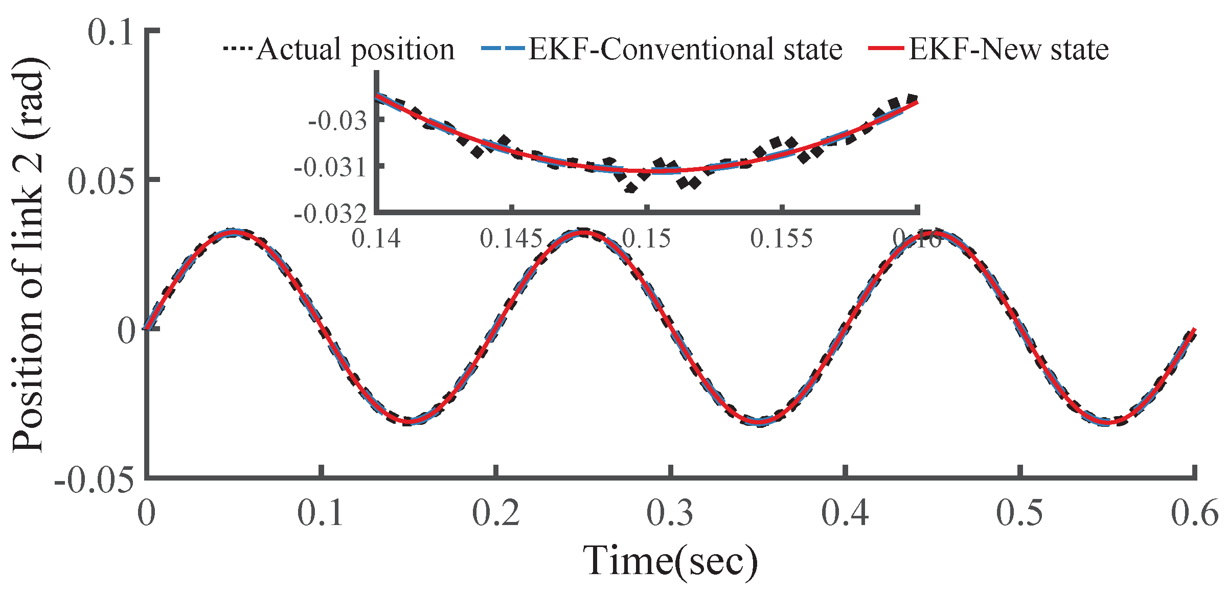
Figure 8 and Figure 9 (where the two EKFs are named as EKF-Conventional state and EKF-New state for short) show the estimation results of the two EKFs for each link position. In Table 1, the RMS value is defined as root mean square of the estimation (tracking) error on a trip of time T ( T = 0.6 s). The Computation period is the average time cost by EKF computing for the two links in every sampling period (closed-loop cycle), on a laptop platform equipped with Intel(R) Core(TM) i3 CPU M 380 @ 2.53 GHz, 4GB RAM, 32-bit Windows OS.
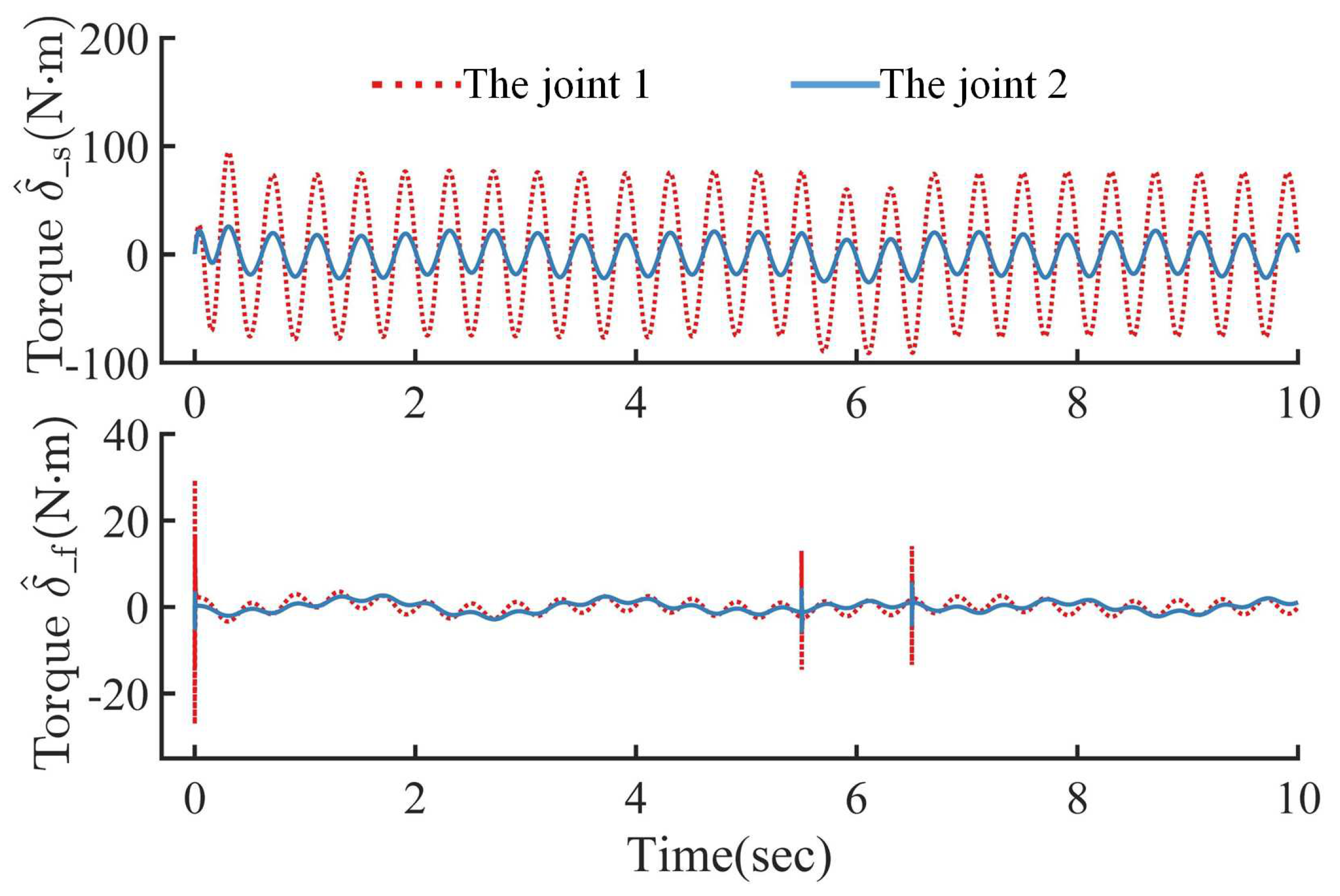
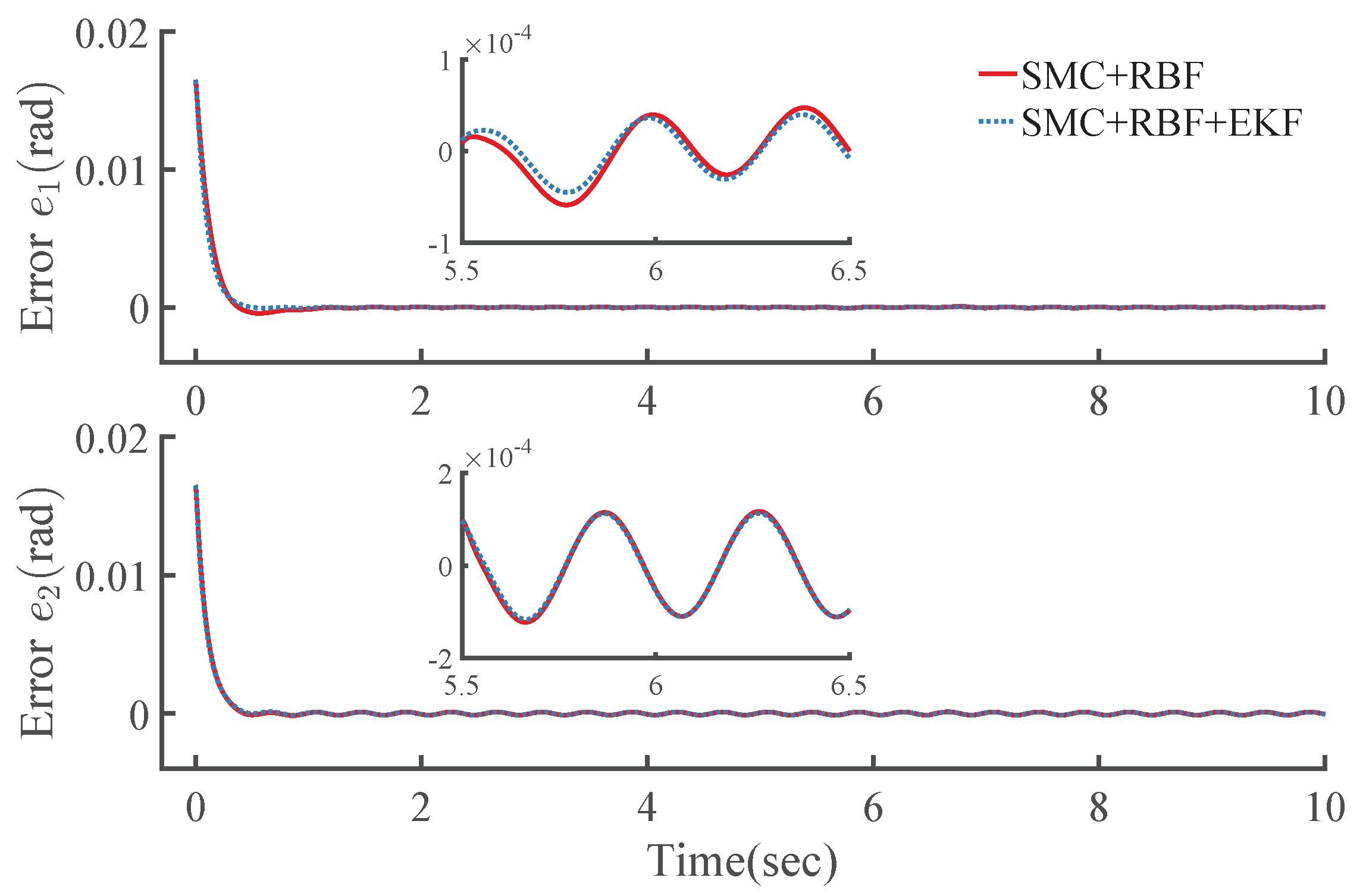
The RMS values of the two EKF observers are very close to each other, both of them are qualified to implement the observation with nearly equal dynamic performance. The computation period is shortened from 6.8 to 5.0 ms, and the efficiency increased by about 26%. That is, the proposed EKF is more efficient and requires a shorter computation period, but without sacrificing the observation accuracy. Such a result was confirmed by large amounts of tests with other different trajectories. As shown in Figure 10 and Figure 11, the controller involving the EKF-New state (named as SMC + RBF + EKF) can achieve almost the same control performance as the controller SMC + RBF, and it can also alleviate the torque vibration caused by chattering to a certain degree.

7.3. Controller Performance Comparisons

To evaluate the proposed scheme in presence of dynamics uncertainties and joint torque disturbances, comparisons with the other two controllers are made. The controller in [37] is a combination of the nonlinear feedforward control and the linear singular perturbation control (named as SPC-FFC). Controller SMC+DO is the proposed controller SMC combined with the disturbance observer in [38].
To perform overall quantitative evaluation of the controllers, together with the previously mentioned RMS value, we adopt another four criteria defined in [39]: Adjusting time, Recovery time, Steady-state error and Maximum deviation.
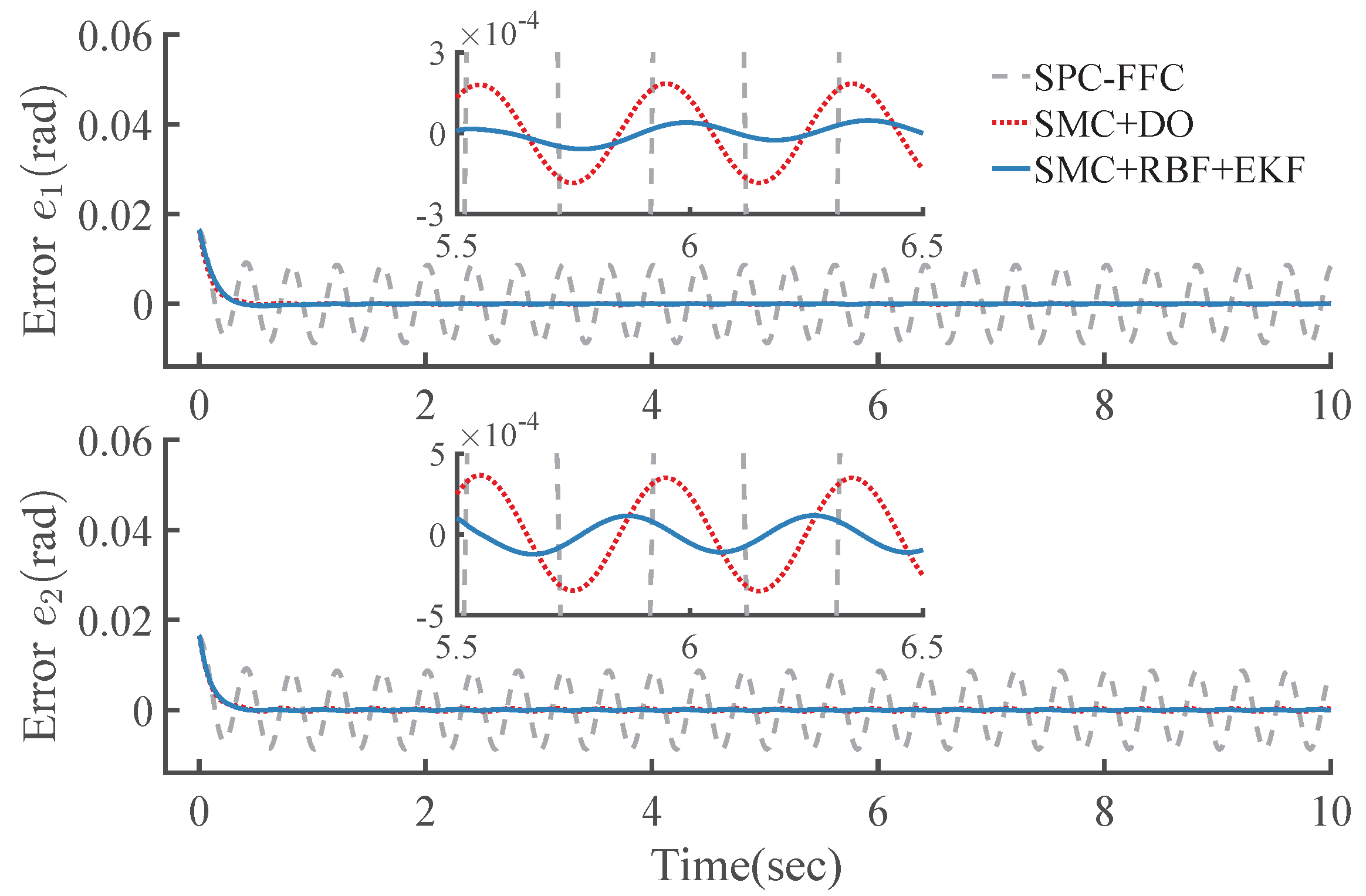
As shown in Figure 12, in the presence of model uncertainties and joint torque disturbances, the controller SPC+FFC with a feedforward term based on the accurate model, presents a lower tracking accuracy than the other two controllers of SMC type. Due to the feedforward compensation based on a disturbance observer, the switching gain of the controller SMC+DO required needs to be set larger than the upper bound of the disturbance estimation error, and thus that the tracking accuracy and strong robustness of the controller as well as chattering attenuation can all be guaranteed.
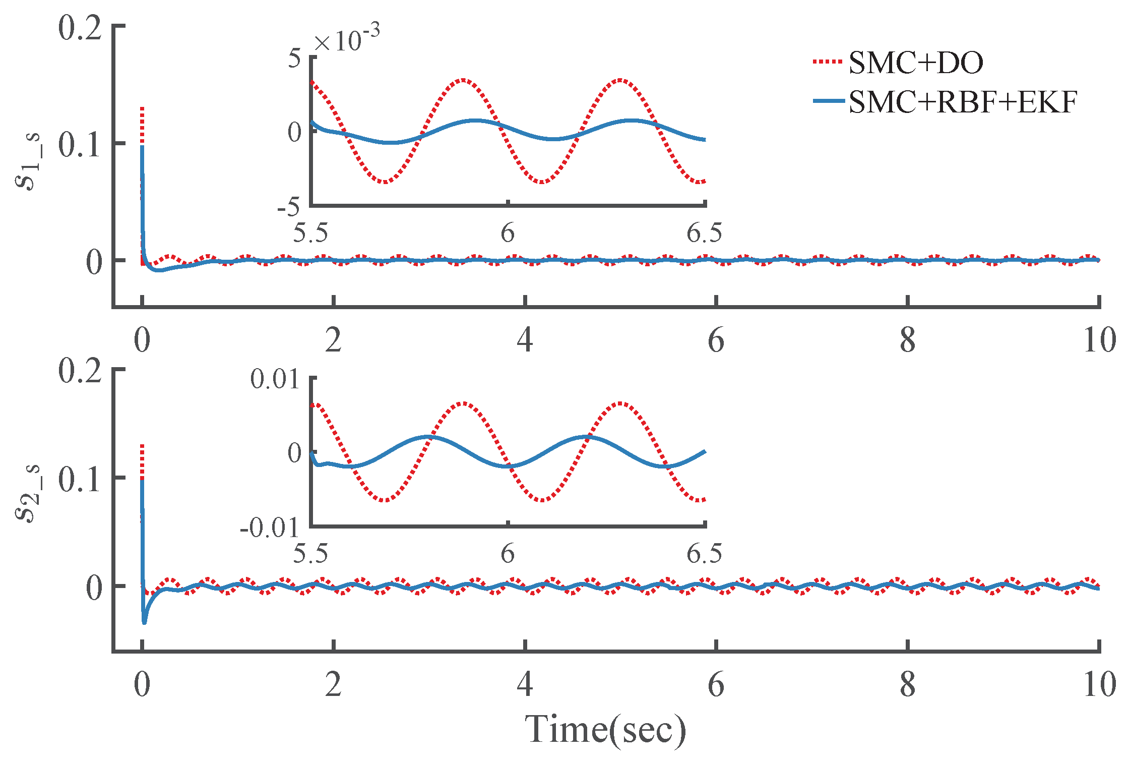
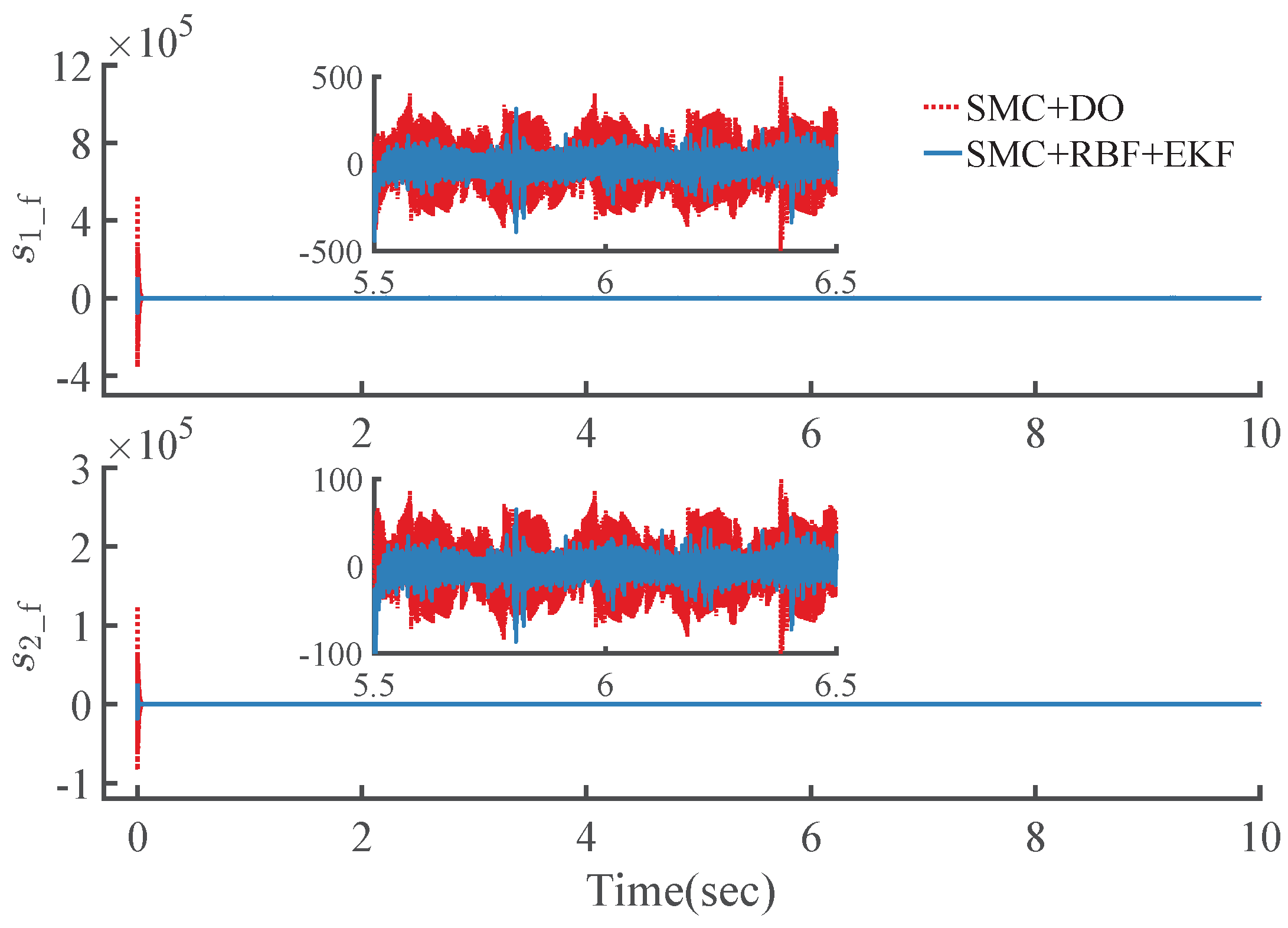
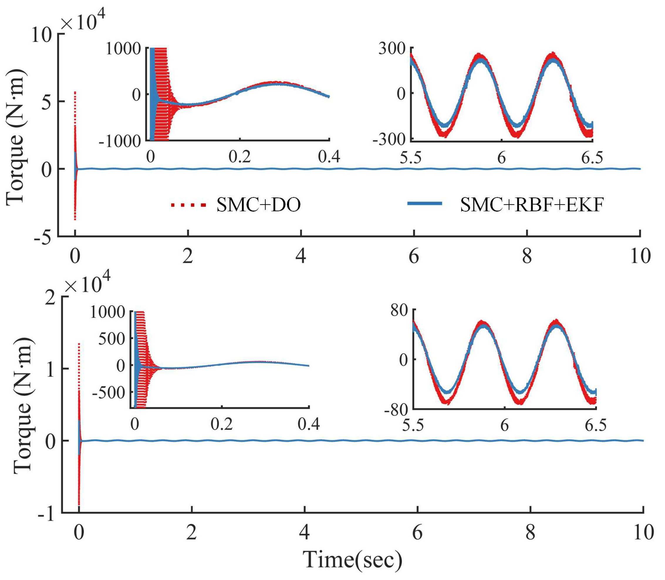
As shown in Figure 12, Figure 13, Figure 14 and Figure 15 and Table 2, with the feedforward torque compensation caused by the proposed RBF compensator based on tracking error, the proposed controller SMC+RBF+EKF cannot only achieve superior performance similar to that of the controller SMC+DO, but also can improve the dynamic performance of the control system, with shorter adjusting time and recovery time, and smaller maximum deviation, steady-state error and RMS value, as well as better chattering attenuation. Furthermore, state measurements of links are eliminated.
Remark 10.
The simulation results obtained above can provide a priori judgments on real experiments. In particular, this has important guiding significance for the practical application of SMC and for addressing its chattering problem. Furthermore, the proposed controller with EKF-New state provides a feasible solution for these robots without sensors on the link side to achieve the closed-loop tracking control with neither position nor velocity measurements of links, instead of consuming large amounts of hardware transformation costs.

8. Conclusions

This paper discusses sliding mode control and its chattering suppressing method for flexible-joint robot manipulators with neither position nor velocity measurements of links, within the frame of the singular perturbation theory. We have shown that, within the framework of singular perturbation theory, the slow and the fast subsystems are transformed into two typical tracking systems without calculating Z ¨ or η ¨ . The slow subsystem is to make q track q d , while the fast is to make Z track h 0 . This makes the controller design easy and flexible. Furthermore, asymptotic stability of the whole control system is proved by comprehensive and strict analysis.
The EKF with respect to a new state variable simplifies calculating the Jacobian matrix, and is validated to be qualified to observe the position and velocity of links, with a nearly equal dynamic performance with higher computing efficiency, in comparison to the EKF with conventional state variable. After the smooth-saturation-function-contained reaching law is dedicated in a proactive way to alleviate the inherent chattering internally in the proposed SMC, online operational RBFNN-based soft computing as an external chattering-suppressed method is validated to be effective to avoid requiring large switching gain to cover the upper bound of the lumped uncertainties that may cause severe chattering. This enables a superior dynamic performance without state measurements of links for the proposed approach than the benchmark controllers with full-state feedback.
Experimental verification of the proposed SMC on physical platform will be pursued in future work. Furthermore, future researches can attempt to extend the proposed SMC with an NN-based soft computing strategy to robots via a data-driven way that is model-free to, thus, omit the complicated process of identification and verification of model parameters.
Author Contributions

Conceptualization, X.C. and H.L.; methodology, X.C., H.L. and W.L.; software, X.C. and H.L.; validation, X.C. and H.L.; formal analysis, X.C. and H.L.; investigation, X.C.; resources, H.L.; writing-original draft X.C.; writing-review and editing, X.C., H.L. and W.L.; supervision, H.L.; project administration, H.L.; funding acquisition, H.L. All authors have read and agreed to the published version of the manuscript.

Funding

The authors disclosed receipt of the following financial support for the research, authorship, and/or publication of this article: The Shanghai Rising-Star Program under Grant 19QA1400400, the Natural Science Foundation of Shanghai under Grant 21ZR1401100, the Fundamental Research Funds for the Central Universities under Grant 2232020G-09 and the Graduate Student Innovation Fund of Donghua University under Grant CUSF-DH-D-2021052.

Institutional Review Board Statement

Not applicable.

Informed Consent Statement

Not applicable.

Data Availability Statement

Not applicable.

Conflicts of Interest

The authors declared no potential conflicts of interest with respect to the research, authorship, and/or publication of this article.

Nomenclature

EKFExtended Kalman Filter
FFCFeedforward Control
NNNeual Network
PDProportional Derivative
RBFNNRadial Basis Function Neural  Network
RMSRoot Mean Square
SMCSliding Mode Controller
SPCSingular Perturbation Control

References

  1. Spong, M.W. Modeling and control of elastic joint robots. ASME J. Dyn. Syst. Meas. Control 1987, 109, 310–319. [Google Scholar] [CrossRef]
  2. Choi, J.; Hong, S.; Lee, W.; Kang, S.; Kim, M. A Robot Joint with Variable Stiffness Using Leaf Springs. IEEE Trans. Robot. 2011, 27, 229–238. [Google Scholar] [CrossRef]
  3. Kammogne, A.S.T.; Kountchou, M.N.; Kengne, R.; Azar, A.T.; Fotsin, H.B.; Ouagni, S.T.M. Polynomial robust observer implementation based passive synchronization of nonlinear fractional-order systems with structural disturbances. Front. Inf. Technol. Electron. Eng. 2020, 21, 1369–1386. [Google Scholar] [CrossRef]
  4. Yilmaz, B.M.; Tatlicioglu, E.; Savran, A.; Alci, M. Adaptive fuzzy logic with self-tuned membership functions based repetitive learning control of robotic manipulators. Appl. Soft Comput. 2021, 104, 107–183. [Google Scholar] [CrossRef]
  5. Nguyen, M.H.; Dao, H.V.; Ahn, K.K. Active disturbance rejection control for position tracking of electro-hydraulic servo systems under modeling uncertainty and external load. Actuators 2021, 10, 20. [Google Scholar] [CrossRef]
  6. Lu, Z. Iterative learning control algorithm for optimal path industrial manipulator. J. Intell. Fuzzy Syst. 2021, 40, 5875–5882. [Google Scholar] [CrossRef]
  7. Yeh, Y.L. Output feedback tracking sliding mode control for systems with state and input dependent disturbances. Actuators 2021, 10, 117. [Google Scholar] [CrossRef]
  8. Hamzeh, N.F.; Fayazi, A.; Ghayoumi, Z.H.; Fatehi, M.H.; Hosseinnia, S.H. Precise tip-positioning control of a single-link flexible arm using a fractional-order sliding mode controller. J. Vib. Control 2020, 26, 1683–1696. [Google Scholar] [CrossRef]
  9. Shtessel, Y.; Edwards, C.; Fridman, L.; Levant, A. Sliding Mode Control and Observation; Springer: New York, NY, USA, 2014. [Google Scholar]
  10. Liu, C.; Wen, G.; Zhao, Z.; Sedaghati, R. Neural-network-based sliding-mode control of an uncertain robot using dynamic model approximated switching gain. IEEE Trans. Cybern. 2020, 51, 1–8. [Google Scholar] [CrossRef] [PubMed]
  11. Yeh, Y.L. A robust noise-free linear control design for robot manipulator with uncertain system parameters. Actuators 2021, 10, 121. [Google Scholar] [CrossRef]
  12. Baek, J.; Kwon, W.; Kim, B.; Han, S. A Widely Adaptive Time-Delayed Control and Its Application to Robot Manipulators. IEEE Trans. Ind. Electron. 2019, 66, 5332–5342. [Google Scholar] [CrossRef]
  13. Baek, J.; Cho, S.; Han, S. Practical Time-Delay Control With Adaptive Gains for Trajectory Tracking of Robot Manipulators. IEEE Trans. Ind. Electron. 2018, 65, 5682–5692. [Google Scholar] [CrossRef]
  14. Nicolis, D.; Allevi, F.; Rocco, P. Operational Space Model Predictive Sliding Mode Control for Redundant Manipulators. IEEE Trans. Robot. 2020, 36, 1348–1355. [Google Scholar] [CrossRef]
  15. Mo, H.; Wei, R.; Ouyang, B.; Xing, L.; Shan, Y.; Liu, Y.; Sun, D. Control of a Flexible Continuum Manipulator for Laser Beam Steering. IEEE Robot. Autom. Lett. 2021, 6, 1074–1081. [Google Scholar] [CrossRef]
  16. Wang, H.; Pan, Y.; Li, S.; Yu, H. Robust Sliding Mode Control for Robots Driven by Compliant Actuators. IEEE Trans. Control. Syst. Technol. 2019, 27, 1259–1266. [Google Scholar] [CrossRef]
  17. Zhang, Z.; Leibold, M.; Wollherr, D. Integral sliding-mode observer-based disturbance estimation for Euler-Lagrangian systems. IEEE Trans. Control Syst. Technol. 2019. [Google Scholar] [CrossRef] [Green Version]
  18. Huang, J.; Ri, S.; Fukuda, T.; Wang, Y. A Disturbance Observer Based Sliding Mode Control for a Class of Underactuated Robotic System With Mismatched Uncertainties. IEEE Trans. Autom. Control 2019, 64, 2480–2487. [Google Scholar] [CrossRef]
  19. Yu, X.; Kaynak, O. Sliding-mode control with soft computing: A survey. IEEE Trans. Ind. Electron. 2009, 56, 3275–3285. [Google Scholar]
  20. Liu, H.S.; Huang, Y. Bounded adaptive output feedback tracking control for flexible-joint robot manipulators. J. Zhejiang Univ.-Sci. A 2018, 19, 557–578. [Google Scholar] [CrossRef]
  21. Khalil, H.K.; Praly, L. High-Gain Observers in Nonlinear Feedback Control. Int. J. Robust Nonlinear Control 2014, 24, 993–1015. [Google Scholar] [CrossRef]
  22. Zhou, Y.; Soh, Y.; Shen, J. High-gain observer with higher order sliding mode for state and unknown disturbance estimations. Int. J. Robust Nonlinear Control 2014, 24, 2136–2151. [Google Scholar] [CrossRef]
  23. Lightcap, C.A.; Banks, S.A. An extended Kalman filter for real-time estimation and control of a rigid-link flexible-joint manipulator. IEEE Trans. Control Syst. Technol. 2010, 18, 91–103. [Google Scholar] [CrossRef]
  24. He, W.; Huang, B.; Dong, Y.; Li, Z.; Su, C.Y. Adaptive neural network control for robotic manipulators with unknown deadzone. IEEE Trans. Cybern. 2018, 48, 2670–2682. [Google Scholar] [CrossRef] [PubMed]
  25. Liu, J.K. Sliding Mode Control Design and Matlab Simulation; Tsinghua University Press: Beijing, China, 2005. [Google Scholar]
  26. Bai, W.; Zhou, Q.; Li, T.; Li, H. Adaptive reinforcement learning neural network control for uncertain nonlinear system with input saturation. IEEE Trans. Cybern. 2020, 50, 3433–3443. [Google Scholar] [CrossRef] [PubMed]
  27. Spong, M.W.; Khorasani, K.; Kokotovic, P.V. An integral manifold approach to the feedback control of flexible joint robots. IEEE J. Robot. Autom. 1987, 3, 291–300. [Google Scholar] [CrossRef]
  28. El-Badawy, A.A.; Mehrez, M.W.; Ali, A.R. Nonlinear modeling and control of flexible-link manipulators subjected to parametric excitation. Nonlinear Dyn. 2010, 62, 769–779. [Google Scholar] [CrossRef]
  29. Khosravi, M.A.; Taghirad, H.D. Dynamic modeling and control of parallel robots with elastic cables: Singular perturbation approach. IEEE Trans. Robot. 2014, 30, 694–704. [Google Scholar] [CrossRef]
  30. Liu, H.S.; Lai, X.B.; Wu, W.X. Time-optimal and jerk-continuous trajectory planning for robot manipulators with kinematic constraints. Robot. Comput.-Integr. Manuf. 2013, 29, 309–317. [Google Scholar] [CrossRef]
  31. Fallaha, C.J.; Saad, M.; Kanaan, H.Y.; Al-Haddad, K. Sliding-mode robot control with exponential reaching law. IEEE Trans. Ind. Electron. 2011, 58, 600–610. [Google Scholar] [CrossRef]
  32. Liu, H.S.; Hao, K.R.; Lai, X.B. Fuzzy saturated output feedback tracking control for robot manipulators: A singular perturbation theory based approach. Int. J. Adv. Robot. Syst. 2011, 8, 43–53. [Google Scholar] [CrossRef]
  33. Orr, M.J.L. Introduction to Radial Basis Function Networks; Technical Report; Institute for Adaptive and Neural Computation, Edinburgh University: Edinburgh, UK, 1996. [Google Scholar]
  34. Krzywanski, J.; Fan, H.; Feng, Y.; Shaikh, A.R.; Fang, M.; Wang, Q. Genetic algorithms and neural networks in optimization of sorbent enhanced H2 production in FB and CFB gasifiers. Energy Convers. Manag. 2018, 171, 1651–1661. [Google Scholar] [CrossRef]
  35. Krzywanski, J.; Sztekler, K.; Bugaj, M.; Kalawa, W.; Grabowska, K.; Chaja, P.R.; Sosnowski, M.; Nowak, W.; Mika, U.; Byku, S. Adsorption chiller in a combined heating and cooling system: Simulation and optimization by neural networks. Bull. Pol. Acad. Sci. Tech. Sci. 2021, 69. [Google Scholar] [CrossRef]
  36. Reif, K.; Sonnemann, F.; Unbehauen, R. An EKF-based nonlinear observer with a prescribed degree of stability. Automatica 1998, 34, 1119–1123. [Google Scholar] [CrossRef]
  37. Kim, J.; Croft, E.A. Full-state tracking control for flexible joint robots with singular perturbation techniques. IEEE Trans. Control Syst. Technol. 2019, 27, 63–73. [Google Scholar] [CrossRef]
  38. Gao, G.Q.; Ye, M.Y.; Zhang, M.C. Synchronous robust sliding mode control of a parallel robot for automobile electro-coating conveying. IEEE Access 2019, 7, 85838–85847. [Google Scholar] [CrossRef]
  39. Liu, H.S.; Huang, Y. Robust adaptive output feedback tracking control for flexible-joint robot manipulators based on singularly perturbed decoupling. Robotica 2018, 36, 822–838. [Google Scholar] [CrossRef]
Figure 1. Online operational structure of the RBFNN.
Actuators 10 00288 g001
Figure 2. Block diagram of the proposed controller.
Actuators 10 00288 g002
Figure 3. Model of the flexible-joint robot manipulator.
Actuators 10 00288 g003
Figure 4. Trajectory tracking error e .
Actuators 10 00288 g004
Figure 5. Time history of the slow sliding surface s _ s .
Actuators 10 00288 g005
Figure 6. Time history of the fast sliding surface s _ f .
Actuators 10 00288 g006
Figure 7. RBF compensation of torque input.
Actuators 10 00288 g007
Figure 8. Position estimated by EKF of link 1.
Actuators 10 00288 g008
Figure 9. Position estimated by EKF of link 2.
Actuators 10 00288 g009
Figure 10. Trajectory tracking error e .
Actuators 10 00288 g010
Figure 11. Torque control input.
Actuators 10 00288 g011
Figure 12. Trajectory tracking error e .
Actuators 10 00288 g012
Figure 13. Time history of the slow sliding surface s _ s .
Actuators 10 00288 g013
Figure 14. Time history of the fast sliding surface s _ f .
Actuators 10 00288 g014
Figure 15. Torque control inputs.
Actuators 10 00288 g015
Table 1. Comparison of two EKFs.
EKF-Conventional StateEKF-New State
RMS value ( 10 2  rad) e 1 0.9510.998
e 2 0.9980.934
e 1.3791.367
Computation period (ms)6.85.0
Table 2. Performance comparisons.
SMC + RBF + EKFSMC + DOSPC + FFC
Adjusting time (s)Link 10.7710.9481.377
Link 20.8470.8601.275
Recovery time (s)Link 10.1990.2131.773
Link 20.1870.1911.876
Steady-state error ( 10 4 rad)Link 10.381.822.6
Link 21.13.630.2
Maximum deviation ( 10 4 rad)Link 10.42.239
Link 21.34.372
RMS value (rad) e 1 0.05580.06240.1666
e 2 0.04580.09050.1840
e 0.07210.08590.2072
Publisher’s Note: MDPI stays neutral with regard to jurisdictional claims in published maps and institutional affiliations.