Kinematic Analysis of a Parallel Manipulator Driven by Perpendicular Linear Actuators

Abstract

In this paper, a goniometer-type specimen stage with a linear actuation mechanism mounted on a rotation mechanism is introduced. The linear actuation mechanism was modeled as a spatial parallel manipulator consisting of a moving body, three linear actuators, and an anti-rotation mechanism. The three linear actuators were arranged perpendicular to each other. In the specimen stage, the linear actuators were in ball contact with the surface of a holder designed to hold a specimen. For the parallel manipulator, the ball contact was replaced with two prismatic joints and a spherical joint. The mobility of the manipulator without the anti-rotation mechanism was one degree of freedom greater than the number of actuators. Therefore, the redundant one degree-of-freedom motion was restrained using an anti-rotation mechanism with three rotation joints and two prismatic joints. The inverse and direct kinematics of the goniometer mechanism were derived and verified. In addition, the inverse Jacobian was derived, and local and global performance indices were analyzed by the terms of manipulability and isotropy. Finally, the goniometer-type specimen stage was designed by the global performance indices.

1. Introduction

Compared with a serial manipulator, the parallel manipulator has the advantages of higher accuracy, higher load capacity, higher stiffness, etc. [1] Those advantages have been used to produce numerous versions of parallel manipulators. They include, for example, spatial parallel manipulators with three degrees of freedom (DOF). Such manipulators typically have two tilts and one translation. The mechanisms of the manipulators include 3-PSP joint chains [1], 3-PRS joint chains [2], 3-RRS joint chains [3], and a CapPaMan architecture [4]. In addition, three-DOF translations have been implemented in a Cartesian parallel manipulator [5], DELTA robot [6], and cube manipulators [7].

A parallel manipulator has also been employed with a goniometer-type specimen stage in transmission electron microscopy (TEM) [8,9] to observe and analyze the micro- and nanoscale structures of specimens. In TEM, an electron beam generated from an electron gun passes through electron lenses in a vacuum, penetrates the specimen, and finally is projected on an imaging device.

The goniometer-type specimen stage is mounted outside the column of the TEM and is to supply and manipulate the specimen [10,11]. The specimen stage is composed of actuating systems, an anti-rotation mechanism, and a holder. The actuation systems typically consist of one rotational actuation system and three linear actuation systems. The linear actuator systems are mounted on the rotational actuation system.

The linear actuation system consists of linear actuators, a set of guiding columns including a head, a column, and a pivot-sliding joint, and a holder [12,13]. The linear actuators apply forces to the holder transports a specimen from the ambient atmosphere into the vacuum chamber of a TEM. To perform this transportation, the holder passes through the guide column into a vacuum chamber.

Generally, the motion of the holder tip on the specimen stage requires three translations. However, with existing parallel manipulators, three translations in the specimen stage are not possible, because of the pivot-sliding joint. As the holder passes the pivot-sliding joint, the motion of the holder tip is transformed to tilts and translation.

In a usual goniometer-type specimen stage, the displacements generated from two of the three linear actuators are tilted, contracted, and inverted by a lever mechanism with a pivot-sliding joint in the guide column. As a result, the linear actuation system generates one translation and two tilt motions. The two tilt motions can be approximated as linear motions because of their large rotation radius and small displacement.

The mechanism of the goniometer-type specimen stage has a compact and simple structure. In addition, this mechanism has simple, explicitly formed kinematics. Moreover, this mechanism has the functions of a displacement amplification, as well as a displacement reduction, due to a lever mechanism. In particular, the reduction function leads to a mechanism for precision work in a small workspace. As a result, this manipulator is applicable to a specimen stage in TEM for the precision manipulation of a very small specimen.

Although goniometer-type specimen stage mechanisms are widely used in TEMs, they have not been reported yet. In this paper, a goniometer-type specimen stage is introduced. The specimen stage has a linear actuation mechanism mounted on a rotation mechanism. The linear actuation mechanism in the specimen stage was modeled as a spatial parallel manipulator. The parallel manipulator consisted of a moving body, three linear actuators, and an anti-rotation mechanism. The three linear actuators were arranged perpendicular to each other. The mobility of the parallel manipulator was obtained. The direct and inverse kinematics were derived with explicit forms. In addition, a workspace calculated using direct kinematics was analyzed. The local and global performance indices of manipulability and isotropy were analyzed using the Jacobian of the manipulator. Finally, the goniometer-type specimen stage was designed by the global performance indices.

2. The Structure of a Parallel Manipulator Driven by Three Perpendicular Linear Actuators

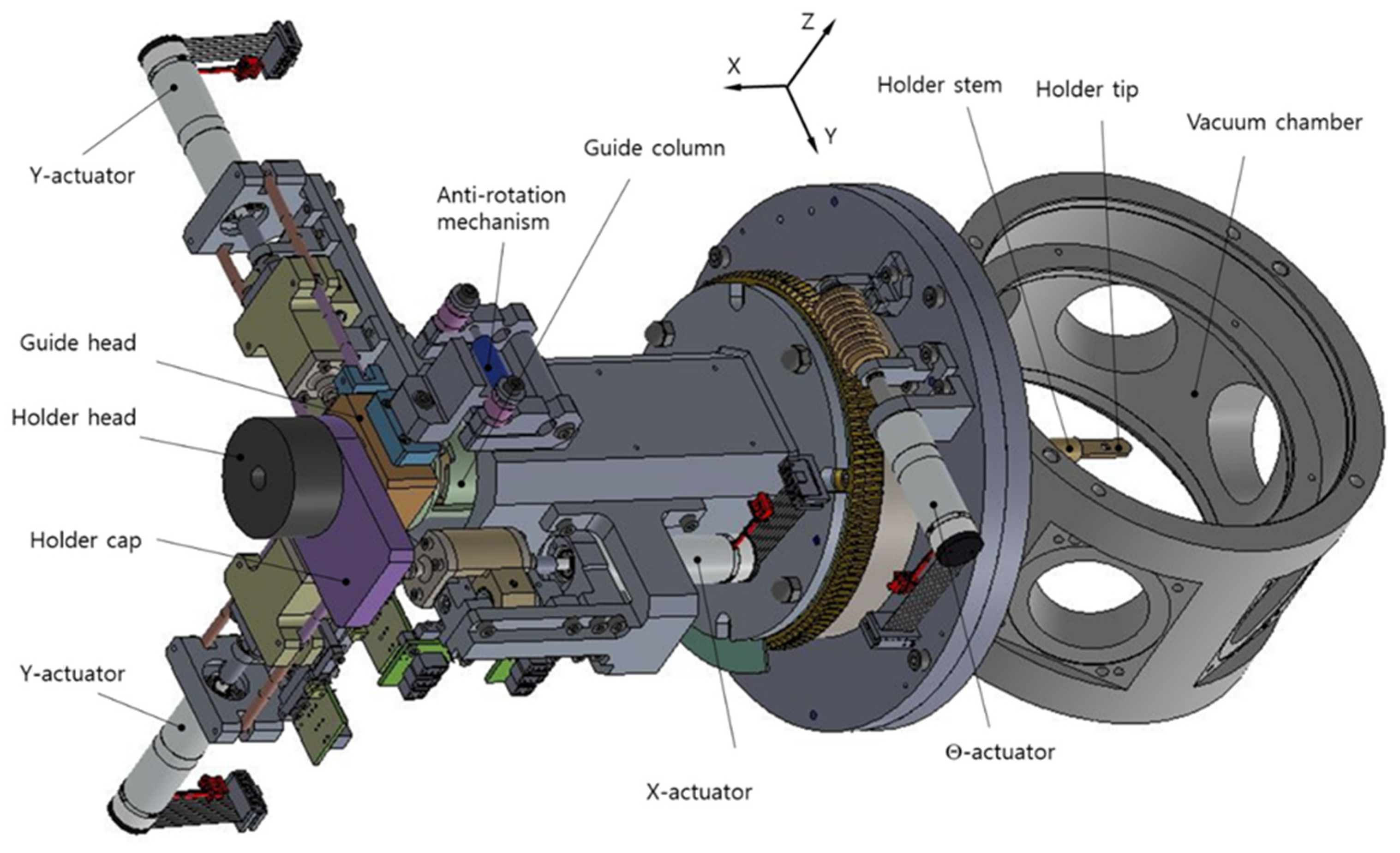
Figure 1 shows the goniometer-type specimen stage designed by our team for a transmission electron microscope (TEM). This specimen stage has four actuators for one rotation and three translations. The linear actuation mechanism with three linear actuators is mounted serially on the rotational mechanism. The Y and Z actuators apply push forces to a guide head for forwarding motion. The backward motion for the Y and Z axes is produced by springs connected between the actuator and the guide head.

The holder consists of a holder head, a holder cap, a holder stem, and a holder tip. The holder passes through the guide head, a guide column, and a pivot-sliding joint into a vacuum chamber. The X actuator pushes the holder cap for forwarding motion. The backward motion of the x axis is produced by the pressure difference between the vacuum chamber and the environment. There is a small hole in the tip of the holder where the sample is placed. An electron beam passes through the hole to inspect the sample. In order to inspect the sample, it is necessary to move the sample along the X, Y, and Z directions using linear actuators. Each linear actuator has a ball tip that is in contact with the guide head or the holder cap. In addition, the mechanism has an anti-rotation mechanism to constrain rotational motion.

The linear actuation mechanism of the goniometer-type specimen stage can be modeled as a spatial parallel manipulator, as shown in Figure 2. Three linear actuators are arranged perpendicular to each other in a Cartesian coordinate system. The moving body consists of a stem and four crossed branches, two of which are folded. Each linear actuator applies force to each branch. The stem passes through the pivot-sliding joint. The linear actuators are connected to the branch through joint chains. The ball contact is replaced with an SPP joint chain, where S and P indicate a spherical joint and a prismatic joint. An anti-rotation mechanism is added to prevent the moving body from rotating. The anti-rotation mechanism is also connected to the branch with a joint chain.

The mobility of the parallel manipulator in Figure 1 can be calculated using the Chebychev–Grübler–Kutzbach criterion [14] as follows:

$$M=6\left(N-1-j\right)+{\displaystyle \sum }_{i=1}^j{f}_i ,$$

(1)

where M is mobility, N is the number of links, j is the number of joints, and f_i is the degree of freedom in the i-th joint. The fixed frame and the moving body each have one link. Each actuating mechanism consists of three links, four joints with six DOF, in which the joints form a PSPP joint chain where P is the linear actuator. The anti-rotation mechanism consists of three links and four joints with five DOF, in which the joints form an R(RP)PR chain, where R is a rotation joint. The (RP) means one joint and two DOF for the rotation and translation. The pivot-sliding joint consists of one link and two joints with four DOF, in which the joints form an SP joint chain.

The mobility of the parallel manipulator without the anti-rotation mechanism is considered. In this case, the number of total links is 12, the number of total joints is 14, and the total degrees of freedom is 22. As a result, the mobility in Equation (1) is four. Since this manipulator has one more mobility than the number of actuators, the motion of one DOF cannot be controlled. There are two choices—one is to add one additional actuator, and the other is to constrain the remaining mobility. Alternatively, the mobility of the goniometer mechanism with the anti-rotation mechanism is considered. In this case, the number of total links is 15, the number of total joints is 18, and the total degrees of freedom is 27. As a result, the mobility is three in Equation (1). Therefore, it is verified that the goniometer mechanism allows three independent motions.

3. Kinematics

Figure 3 shows the skeleton of the parallel manipulator, to help describe the geometrical relations of some points. The dotted skeleton is the initial state of the manipulator, and the solid skeleton is the moving state of the manipulator driven by forces F_X, F_Y, and F_Z. Point O at (0, 0, 0) is the reference point. Point C_O at (h, 0, 0) is the acting point of the forces F_Y and F_Z on the stem. Points A_O and D_O are the initial crossing points of the branches, and they are in the same position (L_1O, 0, 0). Point P_O at (−L_2O, 0, 0) is the initial tip point of the stem. Point B_O at (L_1O, b_Y, 0) is the initial acting point of force F_X.

When forces F_X, F_Y, and F_Z generate the displacement q_X, q_Y, and q_Z, points A_O, B_O, and P_O are transformed to point A at (a_X, a_Y, a_Z), point B at (b_X = L_1O + q_X, b_Y, b_Z = 0), and point P at (p_X, p_Y, p_Z). Points C and D are tilted points with radii h and L_1O from point O of points C_O and D_O due to the forces F_Y and F_Z.

3.1. Inverse Kinematics

Inverse kinematics is used to find the displacements q_X, q_Y, and q_Z when the position of point P is given as (p_X, p_Y, p_Z). Initially, position B (b_X, b_Y, b_Z) and X-directional position h of the Y and Z actuators are given.

In Figure 3, the vector $\overrightarrow{OP}$ is

$$\overrightarrow{OP}=p_X\mathit{i}+p_Y\mathit{j}+p_Z\mathit{k}.$$

(2)

when the length from point O to point A is L₁, and the length from point O to point P is L₂, the total length L_O is

$$L_O=L_{1O}+L_{2O}=L_1+L_2,$$

(3)

where

$$L_2=\sqrt{p_X^2+p_Y^2+p_Z^2}.$$

(4)

Therefore, vector $\overrightarrow{OA}$ is

$$\overrightarrow{OA}=a_X\mathit{i}+a_Y\mathit{j}+a_Z\mathit{k}=-\frac{L_1}{L_2}\left(p_X\mathit{i}+p_Y\mathit{j}+p_Z\mathit{k}\right).$$

(5)

In addition, vector $\overrightarrow{BA}$ is

$$\overrightarrow{BA}=\left(a_X-b_X-q_X\right)\mathit{i}+\left(a_Y-b_Y\right)\mathit{j}+\left(a_Z-b_Z\right)\mathit{k}.$$

(6)

Since vector $\overrightarrow{BA}$ is perpendicular to vector $\overrightarrow{OA}$, the dot product of the vectors is as follows:

$$\overrightarrow{BA}·\overrightarrow{OA}=0.$$

(7)

From Equations (5) and (7), the displacement q_X can be obtained as follows:

$$q_X=-\left(\frac{L_2}{L_1}{p}_X+b_X\right)-\frac{p_Y}{p_X}\left(\frac{L_2}{L_1}{p}_Y+b_Y\right)-\frac{p_Z}{p_X}\left(\frac{L_2}{L_1}{p}_Z+b_Z\right).$$

(8)

Vector $\overrightarrow{O{C}_O}$ is tilted to vector $\overrightarrow{O{C}^{\prime }}$ by the position (p_X, p_Y, p_Z) of the stem tip, as shown in Figure 4. Then, vector $\overrightarrow{O{C}^{\prime }}$ can be derived as follows:

$$\overrightarrow{O{C}^{\prime }}=-\frac{h+\delta }{L_2}\left(p_X\mathit{i}+p_Y\mathit{j}+p_Z\mathit{k}\right).$$

(9)

In addition, the magnitude $\overrightarrow{OC}$ is equal to the magnitude of the vector $\overrightarrow{O{C}_O}$, which is an X-directional component of $\overrightarrow{O{C}^{\prime }}$. Therefore, variable $\delta$ is

$$\delta =-\left(1+\frac{L_2}{p_X}\right)h.$$

(10)

Finally, the displacements of the Y- and Z-directional actuators are

$$\begin{array}{c}{q}_Y=h\frac{p_Y}{p_X},\\ q_Z=h\frac{p_Z}{p_X}.\end{array}$$

(11)

3.2. Direct Kinematics

Direct kinematics is to find the position (p_X, p_Y, p_Z) of the stem tip when the displacements of the actuators are given as (q_X, q_Y, q_Z). As before, position B (b_X, b_Y, b_Z) and the X-directional position h of the Y and Z actuators are given.

As shown in Figure 5, the directional components of point C are

$$\begin{array}{c}{c}_X=\frac{h^2}{\sqrt{h^2+q_Y^2+q_Z^2}} ,\\ c_Y=\frac{h{q}_Y}{\sqrt{h^2+q_Y^2+q_Z^2}} ,\\ c_Z=\frac{h{q}_Z}{\sqrt{h^2+q_Y^2+q_Z^2}}.\end{array}$$

(12)

In addition, in Figure 3, point B is only movable in the x axis direction. When a force F_X causes a displacement q_X, the position of point B becomes (b_X + q_X, b_Y, b_Z). Point C on line $\overline{OA}$ causes the following equation:

$$\frac{a_X-c_X}{c_X}=\frac{a_Y-c_Y}{c_Y}=\frac{a_Z-c_z}{c_Z}=t,$$

(13)

where t is a constant. Using Equations (7) and (13), the position of point A can be found as follows:

$$\begin{array}{c}{a}_X=c_X\frac{c_X\left(b_X+q_X\right)+c_Y{b}_Y+c_Z{b}_Z}{h^2},\\ a_Y=c_Y\frac{c_X\left(b_X+q_X\right)+c_Y{b}_Y+c_Z{b}_Z}{h^2},\\ a_Z=c_Z\frac{c_X\left(b_X+q_X\right)+c_Y{b}_Y+c_Z{b}_Z}{h^2}.\end{array}$$

(14)

In addition, point P on line $\overline{PC}$ causes the following equation:

$$\frac{p_X-c_X}{c_X}=\frac{p_Y-c_Y}{c_Y}=\frac{p_Z-c_z}{c_Z}=s,$$

(15)

where s is constant. From Equation (15), the position (p_X, p_Y, p_Z) can be found as follows:

$$\begin{array}{c}{p}_X=c_X\left(1+s\right)<0,\\ p_Y=c_Y\left(1+s\right),\\ p_Z=c_Z\left(1+s\right).\end{array}$$

(16)

where slope s can be found as follows:

$$s=-1\pm \frac{L_o-L_1}{h}.$$

(17)

and the length L₁ is

$$L_1=\sqrt{a_X^2+a_Y^2+a_Z^2}.$$

(18)

Since physically $L_O>L_1,$ $c_X>0,$ and $h>0$,

$$\begin{array}{c}{p}_X=-\frac{c_X}{h}\left(L_o-L_1\right),\\ p_Y=-\frac{c_Y}{h}\left(L_o-L_1\right),\\ p_Z=-\frac{c_Z}{h}\left(L_o-L_1\right).\end{array}$$

(19)

3.3. Demonstration

The derived kinematics was demonstrated using the output of the direct kinematics as the input of the inverse kinematics and then comparing the output of the inverse kinematics with the input of the direct kinematics, and vice versa. The mechanical parameters used for verification are given in

Table 1. Mechanical parameters.

Parameter	Value (mm)
L1O	232.85
L2O	80.65
h	217.05
bX	232.85
bY	40.0
bZ	0.0

.

Two cases were considered, as shown in

Table 2. Verification of the kinematics.

(a) Case 1
Direct Kinematics				Inverse Kinematics
Input (mm)		Output (mm)		Input (mm)		Output (mm)
qX	10	pX	−68.5	pX	−68.5	qX	10
qY	15	pY	−4.7	pY	−4.7	qY	15
qZ	−10	pZ	3.2	pZ	3.2	qZ	−10
(b) Case 2
Inverse Kinematics				Direct Kinematics
Input (mm)		Output (mm)		Input (mm)		Output (mm)
pX	−50	qX	34.6	qX	34.6	pX	−50
pY	−20	qY	86.8	qY	86.8	pY	−25
pZ	10	qZ	−43.4	qZ	−43.4	pZ	10

. In case 1, the tip position was obtained using the displacements of the actuators from the direct kinematics, and then the displacements of the actuators were obtained using the tip position obtained from the inverse kinematics. As a result, the output displacements in the inverse kinematics were found to be the same as the input displacements in the direct kinematics. In case 2, the displacements of the actuators were obtained using the tip position from the inverse kinematics, and then the tip position was obtained using the obtained displacements of the actuators. As a result, the output tip position was determined to be the same as the input tip position. Therefore, the derived kinematics are valid.

4. Workspace Analysis

The workspace of the parallel manipulator was calculated using Equation (18). The parameters in the direct kinematics are listed in Table 1. A workspace with a set point P was calculated, while q_Y and q_Z were scanned from −100 mm to 100 mm with a q_X of −20, 0, and 20 mm.

The calculated workspace resulted in distorted convex surfaces as shown in Figure 6. The maximum was generated at the point corresponding to the acting point of the X-directional actuator, which was point B.

One point on the workspace was reversed and contracted with respect to displacements q_Y and q_Z of the Y and Z actuators, due to the rotation of the spherical joint and the ratio of the lengths L₁ and L₂. A larger displacement, q_X, of the X actuator caused a shorter length L₂, which resulted in a smaller workspace, as shown in Figure 6a. The workspace was symmetric with respect to the y axis, and was asymmetric with respect to the z axis on the YZ plane, as shown in Figure 6b. As a result, the force acting point of the X actuator eccentric from the center on the YZ plane causes an asymmetric workspace with respect to the z axis.

5. Local Performance Index

The Jacobian matrix plays an important role in the design and analysis of manipulators. Although many studies [15,16,17,18] have performed a kinematic and dynamic analysis based on the Jacobian matrix, this study was limited to kinematic analysis.

Manipulability and isotropy are typical performance indices. In a parallel mechanism, they are calculated using the inverse Jacobian [19]. The inverse Jacobian is defined by

$$J^{-1}=\left[\begin{array}{ccc}\frac{\partial q_X}{\partial p_X}& \frac{\partial q_X}{\partial p_Y}& \frac{\partial q_X}{\partial p_Z}\\ \frac{\partial q_Y}{\partial p_X}& \frac{\partial q_Y}{\partial p_Y}& \frac{\partial q_Y}{\partial p_Z}\\ \frac{\partial q_Z}{\partial p_X}& \frac{\partial q_Z}{\partial p_Y}& \frac{\partial q_Z}{\partial p_Z}\end{array}\right].$$

(20)

In this, the first-row elements can be derived as follows:

$$\begin{array}{c}\frac{\partial q_X}{\partial p_X}=-\frac{1}{L_1}\left(\frac{1}{L_1}+\frac{1}{L_2}\right)\left(p_X^2+p_Y^2+p_Z^2\right)-\frac{L_2}{L_1}\frac{1}{p_X^2}\left(p_X^2-p_Y{}^2-p_Z{}^2\right)+\frac{1}{p_X^2}\left(b_Y{p}_Y+b_Z{p}_Z\right),\\ \frac{\partial q_X}{\partial p_Y}=-\frac{1}{L_1}\left(\frac{1}{L_1}+\frac{1}{L_2}\right)\frac{p_Y}{p_X}\left(p_X^2+p_Y^2+p_Z{}^2\right)-2\frac{L_2}{L_1}\frac{p_Y}{p_X}-\frac{b_Y}{p_X},\\ \frac{\partial q_X}{\partial p_Z}=-\frac{1}{L_1}\left(\frac{1}{L_1}+\frac{1}{L_2}\right)\frac{p_Z}{p_X}\left(p_X^2+p_Y^2+p_Z{}^2\right)-2\frac{L_2}{L_1}\frac{p_Z}{p_X}-\frac{b_Z}{p_X}\end{array}$$

(21)

The second-row elements are as follows:

$$\begin{array}{c}\frac{\partial q_Y}{\partial p_X}=-h\frac{p_Y}{p_X^2},\\ \frac{\partial q_Y}{\partial p_Y}=h\frac{1}{p_X},\\ \frac{\partial q_Y}{\partial p_Z}=0,\end{array}$$

(22)

The third-row elements are as follows:

$$\begin{array}{c}\frac{\partial q_Z}{\partial p_X}=-h\frac{p_Z}{p_X^2},\\ \frac{\partial q_Z}{\partial p_Y}=0,\\ \frac{\partial q_Z}{\partial p_Z}=h\frac{1}{p_X}.\end{array}$$

(23)

5.1. Manipulability

The manipulability [20,21] of a parallel manipulator is defined by

$$w_m=\sqrt{\left|J^{-1}{J}^{-T}\right|} .$$

(24)

where w_m is the manipulability, and J⁻¹ and J^−T are the inverse Jacobian and the inverse transpose Jacobian of this mechanism. The configuration of a manipulator with smaller manipulability means it is near a singularity. Therefore, the configuration of the manipulator requires larger manipulability [20].

Manipulability was calculated while the tip position was scanned along the X, Y, and Z axes. The calculated manipulability exhibited concave-type surfaces, as shown in Figure 7. Three sets of manipulability were obtained, as shown in Figure 7a. As the tip position moved away from the center on the p_Yp_Z plane, the manipulability increased, and the slope of the manipulability increased. In addition, as the X-directional tip position moved away from reference point O, the manipulability decreased. Figure 7b shows the contour map of the top surface in the three manipulability sets. Since the manipulability is symmetric with respect to the Y and Z axes, the manipulability at the center on the p_Yp_Z plane is minimum. The equi-manipulability line is on a circle with its center at p_Y = p_Z = 0.

5.2. Isotropy

The isotropy [22] of the parallel manipulator is defined by

$$w_I=\frac{1}{||J||||J^{-1}||},$$

(25)

where

$$||J||=\sqrt{tr\left(JN{J}^{\mathrm{T}}\right)},$$

(26)

and N is the identity matrix with the n dimension of the Jacobian.

Isotropy was calculated while the tip position was scanned along the X, Y, and Z axes. The calculated isotropy exhibited concave-type surfaces, as shown in Figure 8. Three sets of isotropies were obtained, as shown in Figure 8a. As the tip position moved away from the center on the p_Yp_Z plane, the isotropy increased, and the slope of the isotropy increased; however, the slope of the isotropy became gentler. In addition, as the X-directional tip position moved away from reference point O, isotropy increased and the change of the isotropy became gentler. Figure 8b shows the contour map of the top surface of the three isotropy sets. In Figure 8b, the isotropy is symmetric with respect to the p_Y axis. The minimal isotropy is offset from the center along the p_Y axis on the p_Yp_Z plane where the offset is caused by the eccentric force acting point of the X actuator from the center on the YZ plane along the positive y axis.

6. Application

This parallel manipulator was applied to a goniometer-type specimen stage for TEM. The desired workspace for examining samples in TEM was limited to ±0.5 mm, ±1.5 mm, and ±1.5 mm along the X, Y, and Z axes.

For the design of the parallel manipulator, the force-acting points (B and C) and travel ranges of the linear actuators were chosen as design parameters. The design parameters were limited as follows:

$$\begin{array}{c}35 \mathrm{mm} \le b_Y\le 45 \mathrm{mm},\\ 212 \mathrm{mm}\le h\le 222 \mathrm{mm}.\end{array}$$

(27)

The travel ranges of the X, Y, and Z actuators were calculated by the inverse kinematics within the desired workspace and the constraint (27), and the results are listed in

Table 3. Travel ranges of actuators X, Y, and Z.

Actuator	Travel Range (mm)
X	−1.306~1.396
Y	−4.155~4.155
Z	−4.155~4.155

.

Global performance index means the average of the local performance index over the entire workspace. Therefore, global manipulability W_M and global isotropy W_I can be expressed as follows:

$$\begin{array}{c}{W}_M=\frac{\int w_{M}dV}{\int dV},\\ W_I=\frac{\int w_{I}dV}{\int dV},\end{array}$$

(28)

where V is the volume of the workspace. In general, larger W_M and W_I are preferable. The calculated global manipulability and global isotropy are shown in Figure 9. The global manipulability in Figure 9a increases with h but is independent of b_Y. The global isotropy in Figure 9b decreases with h and b_Y. However, the rate of change for b_Y is about three times greater than for h. The optimal parameters were chosen as the center point of the intersection of the two surfaces, that is, h = 217 mm and b_Y = 40 mm.

The goniometer-type specimen stage was designed with the travel ranges of the actuators and the acting point of the actuators. The motions of Y and Z actuators are reduced by about 2.9 times at the tip. The travel ranges of the actuators were determined by the calculated travel ranges in Table 3, and allowable values were ±2.5 mm, ±7mm, and ±7 mm in the X, Y, and Z actuators. In addition, the optimal parameters were designed by the center point of the intersection of the two surfaces of Figure 9, that is, h = 217 mm and b_Y = 40 mm. Based on the analysis, the goniometer-type specimen stage was developed as shown in Figure 10.

7. Conclusions

In this paper, a goniometer-type specimen stage with a linear actuation mechanism mounted on a rotation mechanism was introduced. The linear actuation mechanism was modeled as a spatial parallel manipulator consisting of a moving body, three linear actuators, and an anti-rotation mechanism. The three linear actuators were arranged perpendicular to each other. In the specimen stage, the linear actuators were in ball contact with the surface of a holder designed to hold a specimen. For the parallel manipulator, the ball contact was replaced with two prismatic joints and a spherical joint. The manipulator analyzed in the terms of mobility, workspace, and local performance indices resulted in the following features:

• Three-DOF mobility;
• Explicit forms of direct and inverse kinematics;
• Distorted convex surface-type workspace with a maximum at the point corresponding to the acting point of the X-directional actuator;
• Concave-type symmetric surfaced local manipulability with the maximum at center with respect to the YZ plane;
• Concave-type surfaced local isotropy with the maximum at an offset distance from the center with respect to the YZ plane.

For the design of the parallel manipulator, the force-acting points and travel ranges of the linear actuators were chosen as design parameters. Based on the workspace analysis, the travel ranges of the linear actuators were determined. In addition, the force contact points were designed as the center point of the intersection of the analyzed global indices. Finally, the goniometer-type specimen stage was developed by the analysis results. The developed goniometer-type specimen stage will be applied in the near future.