An Improved Equivalent-Input-Disturbance Method for Uncertain Networked Control Systems with Packet Losses and Exogenous Disturbances

Abstract

In a networked control system (NCS), time delays, uncertainties, packet losses, and exogenous disturbances seriously affect the control performance. To solve these problems, a modified disturbance suppression configuration of NCS was built. In the configuration, a proportional–integral observer (PIO) reproduces the state of a plant and reduces the observation error; an equivalent input disturbance (EID) estimator estimates and compensates for the disturbance in the control input channel. The stability conditions of the NCS are given by using a linear matrix inequality, and the gains of the PIO and state feedback controller are obtained. Numerical simulation results and an application of a magnetic levitation ball system verifies the effectiveness of the presented method. Comparison with the conventional PIO and EID methods shows that the presented method reduced the tracking error to about one-fifth and two-thirds of their original values, respectively. This demonstrates the validity and superiority of the presented method.

1. Introduction

A networked control system (NCS) has many significant advantages, such as elimination of unnecessary wiring, low cost, and high-reliability [1]. It has been widely used in aerospace, equipment manufacturing, traffic control, and many other fields [2]. However, with the introduction of communication networks, network induced delay and packet loss become unavoidable problems, which reduces the control performance of the system and leads to the instability of the system. In addition, an NCS has a more complex structure and more uncertainties compared with the traditional point-to-point system. It is important to consider the effects of time delay [3], packet losses, exogenous disturbance [4], and uncertainty on system performance in an NCS [5].

Among these problems, stabilizing an NCS is an essential issue and has been widely discussed from different viewpoints [6], for instance, stability analysis [7], state estimation [8], and controller design [9]. An input delay is an important part of induced time-delays in NCSs. It may cause system instability [10,11]. The Smith predictor is an effective approach in handling time delays. An adaptive Smith predictor control problem was investigated in an NCS by incorporating an estimated time delay in the Smith predictor, thus achieving desired tracking performance [12]. A modified Smith predictor combined with a fuzzy model predictive control (FMPC) overcomes the stabilization problem in an NCS [13]. The Smith estimator controller finds it difficult to apply the Smith estimator to the unstable and disturbed networked control system, though it could compensate for constant delay and improve the control performance of an NCS.

Unreliable network transmission and actuator fault would cause packet losses in the NCS [14]. A method of detecting packet losses from process sensor data directly in an NCS was presented to improve the function of the communication network [15]. A stochastic optimal control is derived to reduce the impact of packet losses on system performance [16]. An output–feedback model-predictive control method was designed for an NCS in the presence of packet losses [17]. Sliding-mode controllers were applied to guarantee control performance for both time delays and packet losses [18,19]. An automatic track-keeping algorithm was used to track the reference input and avoid overshoot [20]. An optimal output tracking control method deals with packet losses and the infinite-horizon [21]. An $H_{\infty }$ consensus was considered in an NCS with random packet losses [22].

The uncertainty of structure and parameters of a networked control system leads to coupling between parameters and fluctuation of system output [23,24]. Robust control provides a control performance index for the uncertainty of the system. A robust output tracking controller of an NCS with uncertainties is presented in [25,26]. A robust sliding mode control method was presented, handling an uncertain NCS with two-channel packet losses [27]. A stabilization problem of uncertain networked control systems was investigated in [28]. Moreover, a networked iterative learning control showing good adaptability to the fluctuation caused by the uncertainty in an NCS was proposed in [29]. The proportional–integral observer (PIO) has good adaptability when the objective is controlled with uncertainty [30,31]. When systems are subject to parameter variations, PIO improves the accuracy of disturbance estimation.

Exogenous disturbances are the other problems in an NCS [32,33]. An adaptive model-based event-triggered control for exogenous disturbances suppression is presented in [34]. Predictive control is widely used to reject disturbances in an NCS [35]. A distributed model predictive algorithm was proposed to suppress an exogenous disturbance [36]. In a delta-domain NCS, an optimal control problem is studied to give the system good disturbance rejection performance [37].

Although the above methods consider the problems which exist in the networked system, they have the problems of low compensation efficiency and a small delay compensation range. Therefore, it is necessary to design an efficient compensation control strategy to ensure the packet losses and disturbance suppression effect and ensure the system tracking control performance in NCS. In this paper, we consider the input and output measurement delays of a networked control system and take packet losses and disturbance as the exogenous disturbances of the system; we analyze the stability criteria of the system considering the time delays and parameter uncertainties. According to the stability criterion, the controller design algorithm is obtained to achieve the effective suppression of exogenous disturbances and packet losses.

The active disturbance rejection method is compensated with the exogenous disturbance in the input channel of a control system [38]. The equivalent-input-disturbance (EID) approach is a typical active disturbance rejection method and has been used to estimate the total effect of disturbances in a delay-free dynamic system [39]. An EID is a signal on the system control input channel, which has the same effect on the output as the actual disturbances do. So, the effect of a time delay, packet losses, and disturbances in an NCS can be described using an EID. The approach has been applied to time-delay systems and showed satisfactory disturbance-rejection ability [40,41,42,43]. Delay-dependent guaranteed-cost control was presented by combining the EID approach with the Smith predictor. However, the study is mainly focused on the derivation of stability conditions; the designed controllers are based on stability conditions. Disturbance rejection performance still needs to be improved.

In this study, a new system configuration is built to make the best use of such a controller on the plant side in a networked control system. In the system configuration, a PIO and an EID estimator are arranged on the plant side to estimate and compensate for packet losses, exogenous disturbances, and uncertainties in a timely fashion, and an internal model controller in the main control room ensures control performance of the main control loop at a high level. In the network, packet losses, uncertainties, and exogenous disturbances are taken to be overall disturbances. The PIO is used to reproduce the state of the controlled object with uncertainties, and the EID estimator is used to estimate the exogenous disturbances on the control input channel. The stability conditions of the time-delay control system are given by using a linear matrix inequality (LMI). The simulation results verify the effectiveness of the presented method. Compared with the conventional PIO and EID methods, some results show that this method is superior. The main contribution and novelty of this study are as follows:

(1)

The uncertainties, time delay, packet losses, and exogenous disturbance which simultaneously exist in NCS are compensated for effectively.

(2)

A full-order proportional–integral observer combined with the EID approach is applied to deal with uncertainties in an NCS. This structure of the proportional–integral observer has two degrees of freedom that ensure satisfactory disturbance-suppression.

(3)

The effect of two delays is equivalent to the input channel for stability analysis. The stability condition is presented for the design of the proportional–integral observer and feedback gains.

This paper is organized as follows: Section 2 analyzes the problem of an NCS and describes the configuration of an NCS with an improved EID estimator. Section 3 proves the stability of NCS and gives the method used to design the controller parameters. Section 4 verifies the method through a numerical simulation and its real application to a magnetic levitation ball system. Finally, Section 5 offers some concluding remarks.

In this paper, I is an identity matrix with a compatible dimension; a symmetric matrix $\left[\begin{array}{cc}M& N\\ N^{\mathrm{T}}& P\end{array}\right]$ is indicated by $\left[\begin{array}{cc}M& N\\ ★& P\end{array}\right]$, and a diagonal matrix $\left[\begin{array}{cc}{Q}_1& 0\\ 0& Q_2\end{array}\right]$ is indicated by $\mathrm{diag}\{Q_1,Q_2\}$.

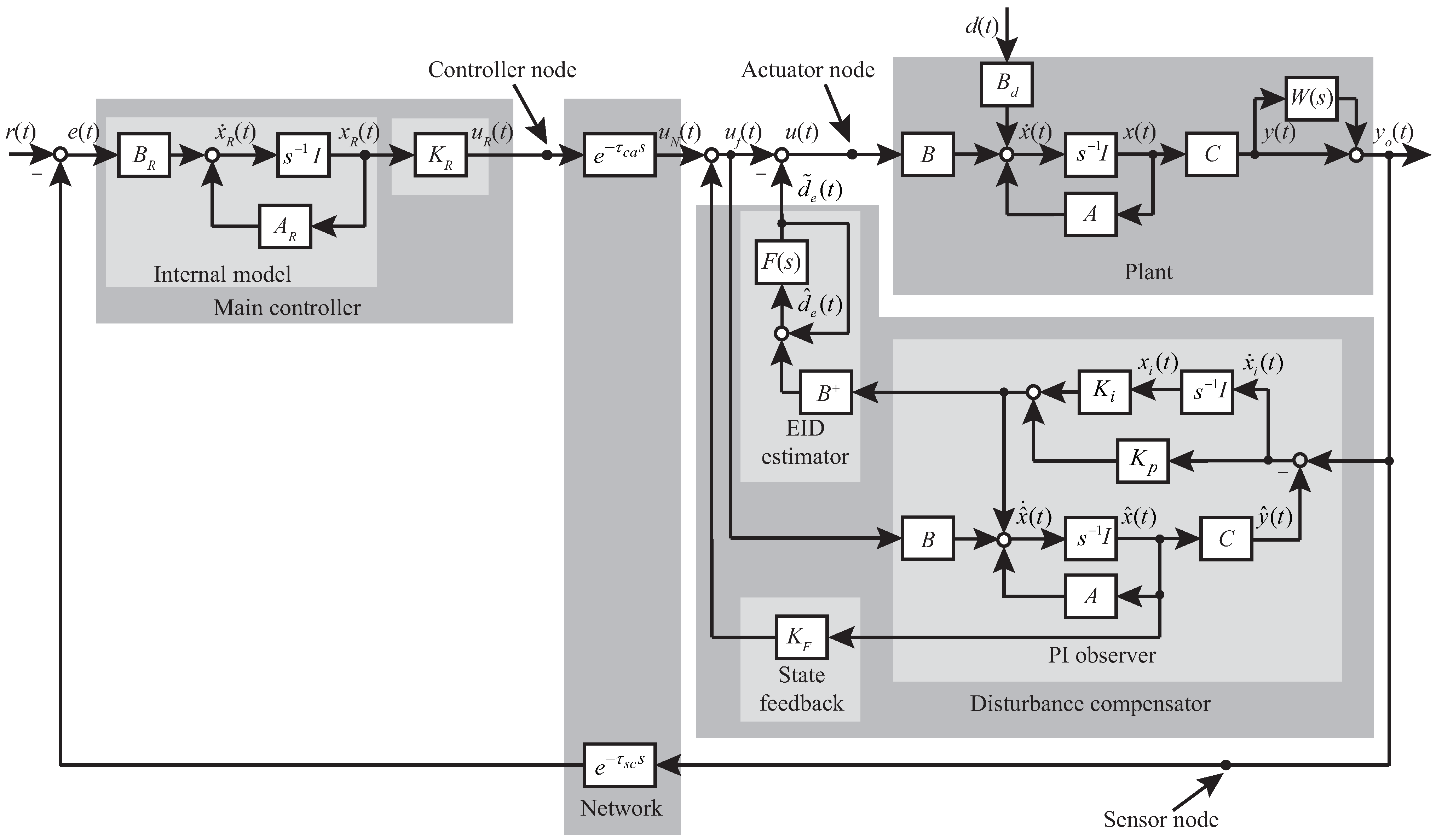
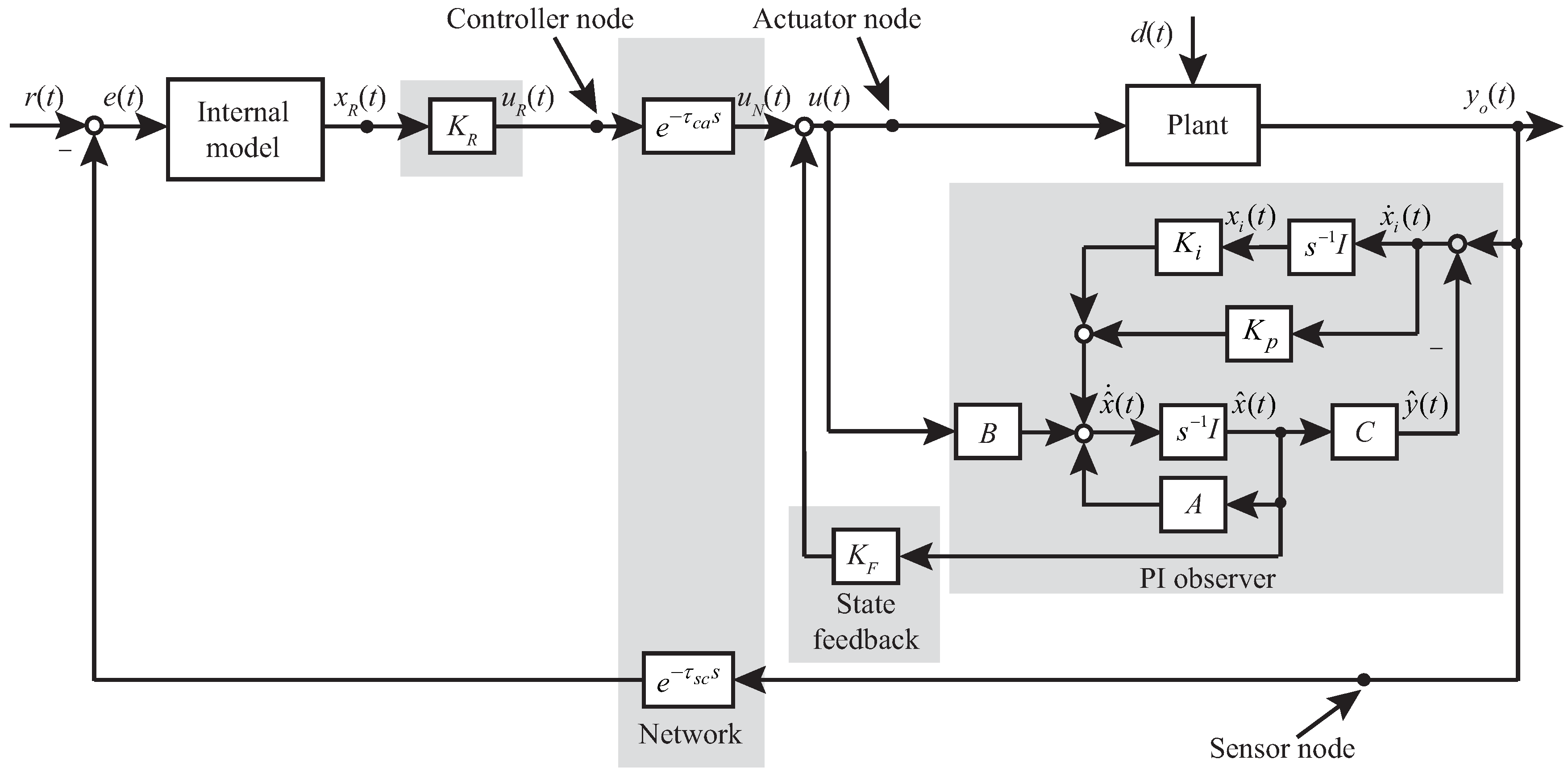
2. Configuration of IEID-Based NCS

The NCS (Figure 1) has a plant, a disturbance compensator, a main controller, and a network. There are two network-induced communication time delays in the network: one from the main controller to an actuator (${\tau }_{ca}$) and one from a sensor to the main controller (${\tau }_{sc}$). Consider the packet losses, uncertainties of the system, and exogenous disturbances. To estimate these effects on the output of the plant, a proportional–integral observer, an improved EID estimator, a state feedback controller, and an internal model controller are established to compensate for these effects. Set the transfer function of the plant to

$$G_p\left(s\right)=(1+W\left(s\right))G_n\left(s\right)$$

(1)

where $W\left(s\right)$ is the weighting function that captures the gain bound of uncertainty. In addition, the nominal part of the plant is $G_n\left(s\right)$. The state-space description of $G_n\left(s\right)$

$$\left\{\begin{array}{c}\dot{x}\left(t\right)=Ax\left(t\right)+\xi \left(t\right)Bu\left(t\right)+B_{d}d\left(t\right)\hfill \\ y\left(t\right)=Cx\left(t\right)\hfill \end{array}\right.$$

(2)

where $u\left(t\right)$, $x\left(t\right)$, and $y\left(t\right)$ are the input, state, and output of the plant, respectively; $d\left(t\right)$ is the overall effect of a bounded exogenous disturbance and packet losses; A, B, $B_d$, and C are constant matrices; and $\xi \left(t\right)$ is the indicator of packet received, that is

$$\xi \left(t\right)=\left\{\begin{array}{c}0,\mathrm{if}\mathrm{the}\mathrm{control}\mathrm{input}\mathrm{is}\mathrm{lost}\mathrm{at}\mathrm{time}t,\hfill \\ 1,\mathrm{if}\mathrm{the}\mathrm{control}\mathrm{input}\mathrm{is}\mathrm{received}\mathrm{at}\mathrm{time}t.\hfill \end{array}\right.$$

(3)

$\xi \left(t\right)$ satisfies the probability distribution

$$\mathrm{Pr}\{\xi \left(t\right)=1\}={\gamma }_0,\mathrm{Pr}\{\xi \left(t\right)=0\}=1-{\gamma }_0.$$

(4)

Decompose the received packet into two parts:

$$\xi \left(t\right)u\left(t\right)=u\left(t\right)+d_{\xi }\left(u\left(t\right)\right)$$

(5)

where $u\left(t\right)$ is the original signal and $d_{\xi }\left(u\left(t\right)\right)$ represents packet losses

$$d_{\xi }\left(u\left(t\right)\right)=[1-\xi \left(t\right)]u\left(t\right).$$

(6)

Assume that

$$|d_{\xi }\left(u\left(t\right)\right)|\le d_{\xi M},\forall t>0$$

(7)

holds for a positive constant $d_{\xi M}$. Assume that $(A,B,C)$ is controllable and observable and has no zeros on the imaginary axis so that it can design a servo control system in the main control loop.

According to the definition of an EID [39], there is an EID, $d_e\left(t\right)$, on the control input channel that has the same effect on the output as $d\left(t\right)$, $d_{\xi }\left(u\left(t\right)\right)$ and uncertainties do. Thus, the original plant (1) can be described as

$$\left\{\begin{array}{c}\dot{x}\left(t\right)=Ax\left(t\right)+B[u\left(t\right)+d_e\left(t\right)]\hfill \\ y_o\left(t\right)=Cx\left(t\right)\hfill \end{array}\right.$$

(8)

where $y_o\left(t\right)$ is the output of the system.

An internal model is used to ensure perfect steady-state tracking. It is

$${\dot{x}}_R\left(t\right)=A_R{x}_R\left(t\right)+B_{R}e\left(t\right)$$

(9)

where $x_R\left(t\right)$ is the state of the main controller. $A_R$ and $B_R$ are the system and input matrices of the internal model. The input signal of that controller is

$$e\left(t\right)=r\left(t\right)-y_o(t-{\tau }_{sc})$$

(10)

where $r\left(t\right)$ is the reference input.

The output of the main controller is

$$u_R\left(t\right)=K_R{x}_R\left(t\right).$$

(11)

A proportional–integral observer is used to reproduce the state of the plant:

$$\left\{\begin{array}{c}\dot{\widehat{x}}\left(t\right)=A\widehat{x}\left(t\right)+K_p[y\left(t\right)-\widehat{y}\left(t\right)]+B{u}_f\left(t\right)+K_i{x}_i\left(t\right)\hfill \\ \widehat{y}\left(t\right)=C\widehat{x}\left(t\right)\hfill \\ {\dot{x}}_i\left(t\right)=y_o\left(t\right)-\widehat{y}\left(t\right)\hfill \end{array}\right.$$

(12)

where $K_p$ and $K_i$ are the observer gains. In addition,

$$u_f\left(t\right)=K_R{x}_R(t-{\tau }_{ca})+K_F\widehat{x}\left(t\right).$$

(13)

A least-squares optimal estimate of the EID is [39]

$${\widehat{d}}_e\left(t\right)=B^{+}\{K_{p}C[x\left(t\right)-\widehat{x}\left(t\right)]+K_i{x}_i\left(t\right)\}+u_f\left(t\right)-u\left(t\right)$$

(14)

where

$$B^{+}={\left(B^{\mathrm{T}}B\right)}^{-1}{B}^{\mathrm{T}}.$$

(15)

In the EID estimator, a first-order low-pass filter, $F\left(s\right)$, is used to suppress high-frequency noise contained in ${\widehat{d}}_e\left(t\right)$:

$${\tilde{D}}_e\left(s\right)=F\left(s\right){\hat{D}}_e\left(s\right)$$

(16)

where ${\tilde{D}}_e\left(s\right)$ and ${\hat{D}}_e\left(s\right)$ are the Laplace transforms of ${\tilde{d}}_e\left(t\right)$ and ${\widehat{d}}_e\left(t\right)$, respectively. The cutoff angular frequency of the filter is usually set to be 5–10 times larger than the highest angular frequency for disturbance rejection. The state-space function of the filter is

$$\left\{\begin{array}{c}{\dot{x}}_F\left(t\right)=A_F{x}_F\left(t\right)+B_F{\widehat{d}}_e\left(t\right)\hfill \\ {\tilde{d}}_e\left(t\right)=C_F{x}_F\left(t\right)\hfill \end{array}\right.$$

(17)

where $A_F$ is stable. As a result, the control input that incorporates an EID estimate is

$$u\left(t\right)=u_f\left(t\right)-{\tilde{d}}_e\left(t\right).$$

(18)

Remark 1.

The uncertainty does not destroy the robust stability of the system. We treat this uncertainty as a disturbance and compensate for it through the presented disturbance-suppression method. The $W\left(s\right)$ in (1) represents an uncertain term. It is a transfer function used in robust control. No matter what form the uncertainty is, it can be suppressed by the disturbance compensation method as long as it does not affect the robust stability.

3. Stability Analysis and System Design of IEID-Based NCS

Time delays in the network make it difficult to stabilize the system and maintain control performance. Since the internal stability of a linear system is independent of exogenous signals, set the reference input and disturbance to be zero. The transfer function from $y\left(t\right)$ to $u_N\left(t\right)$ shows that the effect of two delays is equivalent to a $\tau (={\tau }_{ca}+{\tau }_{sc})$ for stability analysis. Use $\tau$ to rewrite the internal model as

$${\dot{x}}_R\left(t\right)=A_R{x}_R\left(t\right)-B_{R}Cx\left(t\right).$$

(19)

The plant (2) is rewritten as

$$\dot{x}\left(t\right)=Ax\left(t\right)+B[K_R{x}_R(t-\tau )+K_F\widehat{x}\left(t\right)-C_F{x}_F\left(t\right)]$$

(20)

In addition, the proportional–integral observer is rewritten as

$$\dot{\widehat{x}}\left(t\right)=K_{p}Cx\left(t\right)+(A+B{K}_F-K_{p}C)\widehat{x}\left(t\right)+K_i{x}_i\left(t\right)+B{K}_R{x}_R(t-\tau ).$$

(21)

and combining (14) and (17), the low-pass filter is

$${\dot{x}}_F\left(t\right)=(A_F+B_F{C}_F)x_F\left(t\right)+B_F{B}^{+}[K_{p}Cx\left(t\right)-K_{p}C\widehat{x}\left(t\right)+K_i{x}_i\left(t\right)]$$

(22)

Let

$$\chi \left(t\right)={\left[x^{\mathrm{T}}\left(t\right){\widehat{x}}^{\mathrm{T}}\left(t\right)x_i^{\mathrm{T}}\left(t\right)x_F^{\mathrm{T}}\left(t\right)x_R^{\mathrm{T}}\left(t\right)\right]}^{\mathrm{T}}.$$

(23)

Equations (19)–(23) give a state-space description of the IEID control system

$$\dot{\chi }\left(t\right)=\overline{A}\chi \left(t\right)+{\overline{A}}_d\chi (t-\tau )$$

(24)

where $\overline{A}=\left[\begin{array}{ccccc}A& B{K}_F& 0& -B{C}_F& 0\\ K_{p}C& A_F+B{K}_F-K_{p}C& K_i& 0& 0\\ C& -C& 0& 0& 0\\ {\overline{A}}_{41}& -B_F{B}^{+}{K}_{p}C& {\overline{A}}_{43}& {\overline{A}}_{44}& 0\\ -B_{R}C& 0& 0& 0& A_R\end{array}\right],{\overline{A}}_d=\left[\begin{array}{ccccc}0& 0& 0& 0& B{K}_R\\ 0& 0& 0& 0& B{K}_R\\ 0& 0& 0& 0& 0\\ 0& 0& 0& 0& 0\\ 0& 0& 0& 0& 0\end{array}\right],{\overline{A}}_{41}=B_F{B}^{+}{K}_{p}C,{\overline{A}}_{43}=B_F{B}^{+}{K}_i,{\overline{A}}_{44}=A_F+B_F{C}_F.$

When the low-pass filter and internal model controller are known, the PIO and state observer are designed to ensure the stability and disturbance rejection performance of the NCS. There are the lemma and theorem for the design process.

Definition 1.

For a matrix $C\in {\mathbb{R}}^{p\times n}$ that has full row rank, the singular-value decomposition (SVD) of the matrix is

$$C=U\left[S0\right]V^{\mathrm{T}}$$

(25)

where $U\in {\mathbb{R}}^{n\times n}$ and $V\in {\mathbb{R}}^{p\times p}$ are unitary matrices, $S\in {\mathbb{R}}^{n\times n}$ is a semi-positive definite matrix.

Lemma 1

([44]). For the matrix C with the SVD (25), if $\mathrm{\Pi }\in {\mathbb{R}}^{n\times n}$ is a symmetric matrix, then there exists a matrix $\overline{\mathrm{\Pi }}\in {\mathbb{R}}^{p\times p}$ such that $C\mathrm{\Pi }=\overline{\mathrm{\Pi }}C$ holds if and only if

$$\mathrm{\Pi }=V\mathrm{diag}\{{\mathrm{\Pi }}_{11},{\mathrm{\Pi }}_{22}\}{V}^{\mathrm{T}}$$

(26)

where ${\mathrm{\Pi }}_{11}\in {\mathbb{R}}^{p\times p}$ and ${\mathrm{\Pi }}_{22}\in {\mathbb{R}}^{(n-p)\times (n-p)}$.

Lemma 2

(Schur complement [45]). For any real matrix $\mathrm{\Gamma }={\mathrm{\Gamma }}^{\mathrm{T}}$ and $\mathrm{\Gamma }=\left[\begin{array}{cc}{\mathrm{\Gamma }}_{11}& {\mathrm{\Gamma }}_{12}\\ ★& {\mathrm{\Gamma }}_{22}\end{array}\right]$, the following assertion statements are equivalent:

(1)   

$\mathrm{\Gamma }<0$;

(2)   

${\mathrm{\Gamma }}_{11}<0$, ${\mathrm{\Gamma }}_{22}-{{\mathrm{\Gamma }}_{12}}^{\mathrm{T}}{{\mathrm{\Gamma }}_{11}}^{-1}{\mathrm{\Gamma }}_{12}<0$; and

(3)   

${\mathrm{\Gamma }}_{22}<0$, ${\mathrm{\Gamma }}_{11}-{\mathrm{\Gamma }}_{12}{{\mathrm{\Gamma }}_{22}}^{-1}{{\mathrm{\Gamma }}_{12}}^{\mathrm{T}}<0$.

A theorem gives presents a sufficient stability condition of the control system (Figure 1).

Theorem 1.

Set the parameters ${\delta }_1$ and ${\delta }_2$, if there exist appropriate matrices $X_2$, and $W_1$, $W_2$, $W_3$, and $W_4$, and symmetric positive definite matrices $X_1$, $X_{11}$, $X_{22}$, $X_3$, $X_4$, $X_5$, $Y_1$, $Y_2$, $Y_3$, $Y_4$, $Y_5$, and if the following LMI holds, the system (24) is asymptotically stable.

$$\left[\begin{array}{cc}\overline{A}X+X{\overline{A}}^{\mathrm{T}}+Y& {\overline{A}}_{d}X\\ ★& -Y\end{array}\right]<0$$

(27)

where

$$\begin{array}{ccc}& & X=\mathrm{diag}\{{\delta }_1{X}_1,X_2,X_3,X_4,{\delta }_2{X}_5\},\hfill \end{array}$$

(28)

$$\begin{array}{ccc}& & X_2=\mathrm{diag}\{X_{11},X_{22}\},\hfill \end{array}$$

(29)

$$\begin{array}{ccc}& & Y=\mathrm{diag}\{Y_1,Y_2,Y_3,Y_4,Y_5\}.\hfill \end{array}$$

(30)

Moreover, the SVD of C is $U\left[S0\right]{\mathrm{Y}}^{\mathrm{T}}$, where U and Y are unitary matrices, and S is a semi-positive definite matrix.

Let

$$C{X}_1={\overline{X}}_{1}C$$

(31)

and

$${\overline{X}}_1^{-1}=US{X}_{11}^{-1}{S}^{-1}{U}^{\mathrm{T}}.$$

(32)

The gains are given by

$$K_F=W_2{X_2}^{-1},K_R=W_4{X_5}^{-1},K_P=W_{1}US{X}_{11}^{-1}{S}^{-1}{U}^{\mathrm{T}},K_i=W_{3}US{X}_{11}^{-1}{S}^{-1}{U}^{\mathrm{T}}.$$

(33)

Proof. 

A Lyapunov–Krasovskii functional candidate is constructed to be

$$V(\chi \left(t\right),t)={\chi }^{\mathrm{T}}\left(t\right)P\chi \left(t\right)+{\int }_{t-{\tau }_0}^t{\chi }^{\mathrm{T}}\left(s\right)Q\chi \left(s\right)ds$$

(34)

where $P=P^{\mathrm{T}}\ge 0$, $Q=Q^{\mathrm{T}}\ge 0$, and ${\tau }_0\ge 0$ is the upper bound of time delay.

The derivative of $V\left(\chi \right(t),t)$ along the solution of the system (24) is

$$\begin{array}{cc}\hfill \dot{V}(\chi \left(t\right),t)=& 2{\chi }^{\mathrm{T}}\left(t\right)P\overline{A}\chi \left(t\right)+{\chi }^{\mathrm{T}}\left(t\right)Q\chi \left(t\right)+\chi \left(t\right)P{\overline{A}}_d\chi (t-{\tau }_0)\hfill \\ \hfill & +\chi (t-{\tau }_0){\overline{A}}_d^{\mathrm{T}}P\chi \left(t\right)-\chi (t-{\tau }_0)Q\chi (t-{\tau }_0).\hfill \end{array}$$

(35)

Clearly,

$$\begin{array}{c}\hfill \dot{V}(\chi \left(t\right),t)\le {\eta }_1^{\mathrm{T}}\left(t\right)\mathrm{\Xi }{\eta }_1\left(t\right)\end{array}$$

(36)

where ${\eta }_1\left(t\right)={\left[{\chi }^{\mathrm{T}}\left(t\right){\chi }^{\mathrm{T}}(t-{\tau }_0)\right]}^{\mathrm{T}}$ and

$$\mathrm{\Xi }=\left[\begin{array}{cc}P\overline{A}+{\overline{A}}^{\mathrm{T}}P+Q& P{\overline{A}}_d\\ ★& -Q\end{array}\right].$$

(37)

If $\mathrm{\Xi }<0$, then $\dot{V}(\chi \left(t\right),t)<0$ and the system (24) is stable. Let

$$\begin{array}{cc}\hfill & X=P^{-1},Y=P^{-1}Q{P}^{-1}\hfill \end{array}$$

(38)

where

$$\left\{\begin{array}{c}X=\mathrm{diag}\{{\delta }_1{X}_1,X_2,X_3,X_4,{\delta }_2{X}_5\},\hfill \\ X_2=\mathrm{diag}\{X_{11},X_{22}\},\hfill \\ Y=\mathrm{diag}\{Y_1,Y_2,Y_3,Y_4,Y_5\}.\hfill \end{array}\right.$$

(39)

Pre- and post-multiplying the inequality (37) by the matrix $\mathrm{diag}\{P^{-1},I\}$ yields

$$\left[\begin{array}{cc}\overline{A}X+X{\overline{A}}^{\mathrm{T}}+Y& {\overline{A}}_{d}X\\ ★& -Y\end{array}\right]<0.$$

(40)

It is observed that the inequality (40) is not LMI because of the cross terms, for example, $K_F{X}_2$ and $K_R{X}_5$ in $\mathrm{\Lambda }$. Let

$$W_2=K_F{X}_2,W_4=K_R{X}_5.$$

(41)

From Lemma 2, set $C{X}_1={\overline{X}}_{1}C$ where ${\overline{X}}_1$ is an existing matrix. Define

$$W_1=K_p{\overline{X}}_1,W_3=K_i{\overline{X}}_1.$$

(42)

According to the transformation of (41) and (42), (40) is transformed into a standard LMI. Solve this LMI based on the MATLAB toolbox.

For prescribed ${\delta }_1$ and ${\delta }_2$, Solving the LMI (40) provides us the symmetric positive matrices $W_1$, $W_2$, $W_3$, $W_4$, $X_1$, $X_2$, $X_3$, $X_4$, and $X_5$. Combining (41) and (42) yields

$$W_{1}C=K_{p}C{X}_1,W_{3}C=K_{i}C{X}_1.$$

(43)

Combining the singular-value decomposition (SVD) of C, the solution of (43) is

$$K_p=W_{1}US{X}_{11}^{-1}{S}^{-1}{U}^{\mathrm{T}},K_i=W_{3}US{X}_{11}^{-1}{S}^{-1}{U}^{\mathrm{T}},K_F=W_2{X}_2^{-1},K_R=W_4{X}_5^{-1}.$$

(44)

The proof is completed. □

4. Case Study

In this section, a numerical example and a real application of a magnetic levitation ball system are used to verify the effectiveness of the presented method.

4.1. Numerical Example

The numerical example of the plant (2) is [41]

$$A=\left[\begin{array}{cc}-2& 3\\ 4& -5\end{array}\right], B=\left[\begin{array}{c}1\\ 1\end{array}\right], C={\left[\begin{array}{c}2\\ 1\end{array}\right]}^{\mathrm{T}}, B_d=\left[\begin{array}{c}1\\ 1.2\end{array}\right].$$

.

The uncertainties were chosen as

$${\displaystyle W\left(s\right)=\frac{3s+100}{0.1s+200}.}$$

.

In addition, the maximums of the random delays ${\tau }_{ca}$ and ${\tau }_{sc}$ were 0.3 s and 0.1 s (Figure 2), respectively. Thus, the upper bound of $\tau$ was ${\tau }_0=0.4\mathrm{s}$. In the NCS, the probability distribution of packet losses was a random number in the range $[0,0.4]$.

In the NCS, an input reference signal was set to

$$r\left(t\right)=100\times 1\left(t\right)$$

(45)

where $1\left(t\right)$ is the unit step signal.

An exogenous disturbance was

$$d\left(t\right)=30tanh0.1t+50sin0.1\pi t+20cos(0.3/\pi t).$$

(46)

According to the reference (45), the parameters of the internal model (9) were chosen as

$$A_R=-0.001,B_R=1.$$

(47)

Plot an FFT diagram (Figure 3b) of the exogenous disturbance, $d\left(t\right)$ (Figure 3a) to analyze the frequency distribution. The main energy of disturbance is concentrated in the low-frequency band ($\omega <1$ rad/s). Choose the cut-off frequency of the low-pass filter as 10 rad/s and the parameters of the low-pass filter become

$$A_F=-10,B_F=10,C_F=1.$$

(48)

A performance index

$${\displaystyle J_K=\frac{1}{2}{\int }_0^{40}{[r\left(t\right)-y_o\left(t\right)]}^{2}dt}$$

(49)

was used to adjust ${\delta }_1$ and ${\delta }_2$ in LMI (27) so as to find suitable gains of the state feedback and the main controller. Exploring the relationship between $J_K$ and ${\delta }_i(i=1,2)$ using a fixed step searching algorithm gave

$${\delta }_1=24.00,{\delta }_2=0.60.$$

(50)

Solving LMI (27) yielded

$$K_F=[-3.84-0.52],K_R=1.21,K_P={\left[47.56241.99\right]}^{\mathrm{T}},K_i={[123-2.12]}^{\mathrm{T}}.$$

(51)

The simulation results (Figure 4) show that the influence of packet losses and the disturbance are reflected in the estimated EID, ${\tilde{d}}_e\left(t\right)$ (Figure 4a), and then further controls the control input $u\left(t\right)$ (Figure 4b). These ensure that IEID method makes the system stable, and also effectively compensates for packet losses and exogenous disturbances. The effect of the whole disturbance is suppressed to a very low level and the output, $y\left(t\right)$ (Figure 4c), tracks the reference input with a very small tracking error. The steady-state value of the tracking error, $e\left(t\right)$, is only 4; that is, the relative tracking precision is $99.67\%$. Plot the Bode diagram (Figure 4d) from the exogenous disturbance, $d\left(t\right)$ and packet losses to the output, thus analyze the influence of the different-frequencies exogenous disturbance on the output. Figure 4d shows the effectiveness of the control method in the low-frequency band ($\omega <10$ rad/s).

The PIO control method (Figure 5) is widely used in disturbance suppression. A comparison was carried out between the PIO and the presented method. The parameters of the PIO control system were calculated from an LMI, which is a similar method to the presented method. The resulted control gains were

$$K_F=[-21.61-11.73],K_R=1.53,K_P={\left[46.43212.10\right]}^{\mathrm{T}},K_i={[86.43-1.47]}^{\mathrm{T}}.$$

(52)

A comparison with a conventional EID control method [39] is also used to illustrate this feature (Figure 6). The gains of the state-feedback and state observer of the EID control system were

$$K_F=[-3.61-0.73],K_R=1.38,L={\left[5.421.41\right]}^{\mathrm{T}}.$$

(53)

As can be seen in Figure 7a, the output errors of the IEID and the PIO-based NCS indicate that the peak-to-peak value of the tracking errors were 0.89 and 12.14 for the IEID and the PIO control methods, respectively. That is, the presented method reduced the tracking error to less than $7.34\%$ of the PIO control method. From the above discussion, compared with the PIO control method, the IEID method has a better disturbance-suppression ability.

Compared with the conventional EID method, this method has a much shorter transient time and smaller steady-state tracking error, which can be seen from the simulation results (Figure 7b). More specifically, the maximum peak-to-peak value of the steady-state tracking error for the EID control method is 1.28. That is, the IEID control method reduces the tracking error to 69.53% of the EID control method. This proves the effectiveness of the presented method.

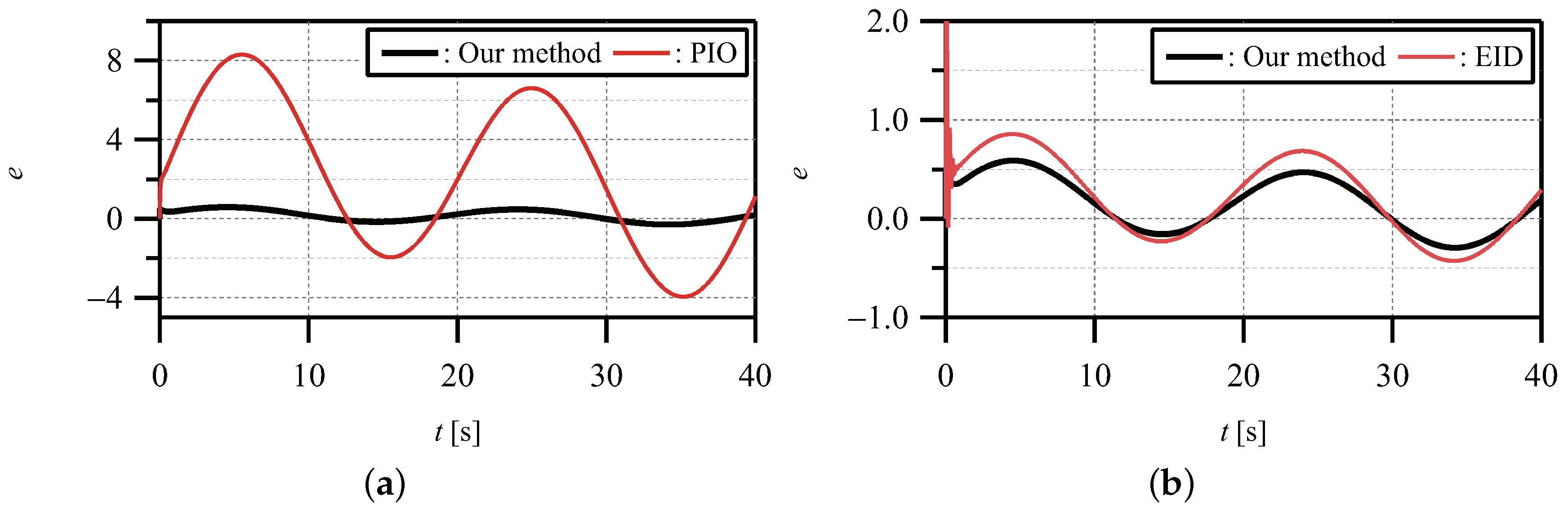
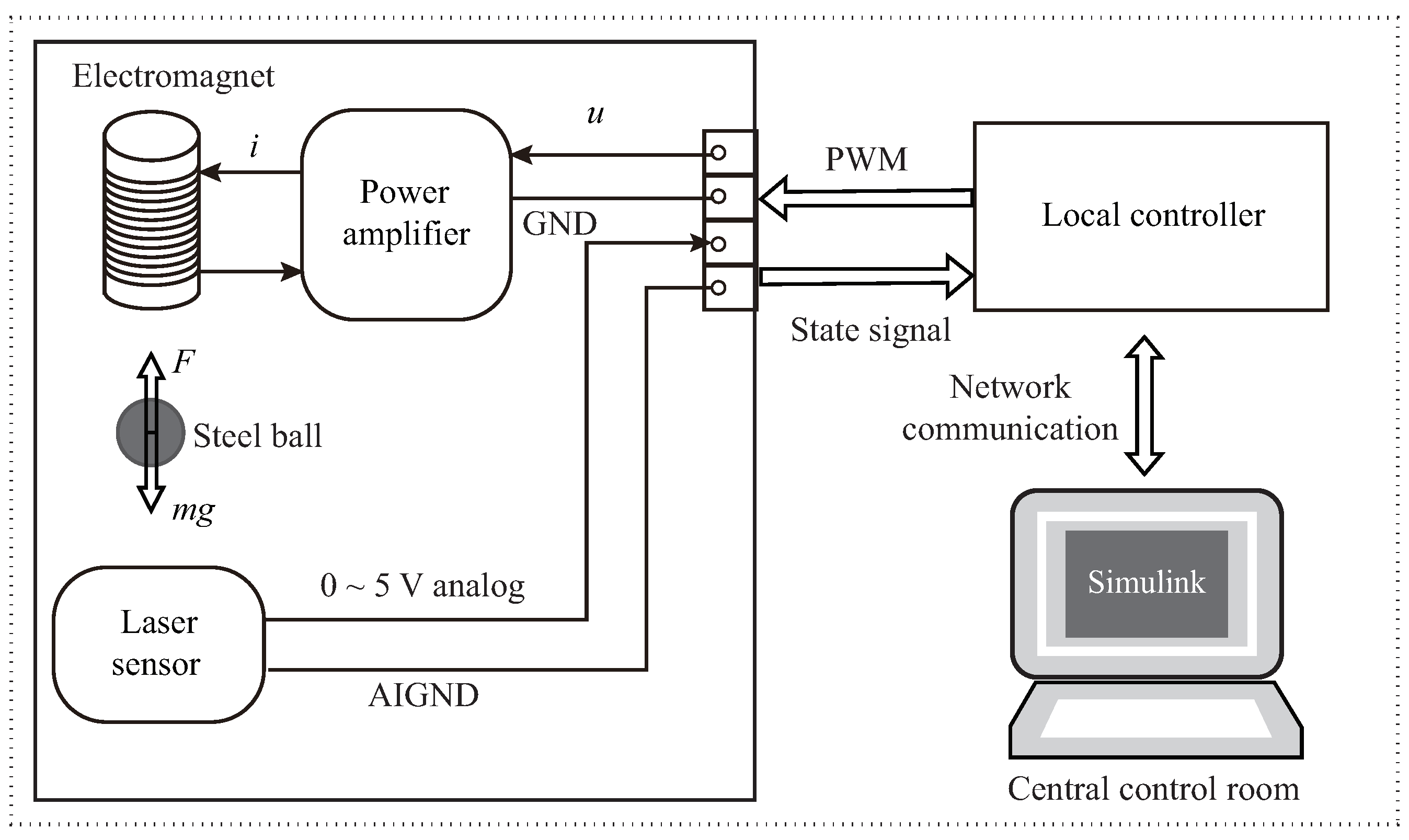
4.2. Example of a Magnetic Levitation Ball System

This study takes a magnetic levitation ball system as an example to further illustrate the effectiveness and applicability of this method [46]. The system (Figure 8) contains an electromagnet, a power amplifier, a laser sensor, a hollow steel ball, a local controller, the main controller, and network communication. The main controller in a central control room carries out high-level control tasks (for example, optimization and intelligent control) and a local feedback controller close to the equipment suppresses disturbances and parameter changes in a timely fashion. The main controller is connected to the plant through the Internet.

For simplicity, we consider a task of the positioning control of the ball in this paper to demonstrate the effectiveness of our method. This system adjusts the current in the electromagnetic coil to stabilize the ball at a prescribed position or drive the ball to track a reference input. The plant considered in this paper is a single-degree-of-freedom magnetic levitation system, in which the ball can only move in the vertical direction. The description and value of symbols are shown in

Table 1. Parameters and variables of the magnetic levitation ball system.

Symbol	Description	Value
m	Mass of steel ball $\left[\mathrm{kg}\right]$	0.17
d	diam of steel ball $\left[\mathrm{m}\right]$	0.06
R	Coil resistance $\left[\mathrm{\Omega }\right]$	13.577
${\mu }_0$	Vacuum permeability $\left[\mathrm{H}/\mathrm{m}\right]$	$4\pi \times {10}^{-7}$
$S_L$	Cross-sectional area of electromagnet magnetic conductivity $\left[{\mathrm{m}}^2\right]$	$9\pi \times {10}^{-4}$
N	Coil turns $\left[\mathrm{Turns}\right]$	1057
$L_R$	Viscous damping coefficient $\left[\mathrm{mH}\right]$	341
$h_0$	Balance position $\left[\mathrm{m}\right]$	0.0425
$i_0$	Balance current $\left[\mathrm{mA}\right]$	0.633
g	Acceleration of gravity $\left[\mathrm{m}/{\mathrm{s}}^2\right]$	9.807
$K_L$	Spring rate $\left[\mathrm{mH}\right]$	–
i	Instantaneous current through the solenoid $\left[\mathrm{mA}\right]$	–
$u\left(t\right)$	Control voltage applied to the solenoid $\left[\mathrm{mV}\right]$	–
$F(i,h)$	Electromagnetic force $\left[\mathrm{N}\right]$	–
h	Gap between the electromagnet surface and steel ball $\left[\mathrm{m}\right]$	–

.

The mathematical model of a magnetic levitation ball system [47] is

$$\left\{\begin{array}{c}{\displaystyle m\frac{d^{2}h}{d{t}^2}=F(i,h)-mg,}\hfill \\ {\displaystyle F(i,h)=K_L{\left(\frac{di}{dt}\right)}^2,K_L=-\frac{{\mu }_0{S}_L{N}^2}{4},}\hfill \\ {\displaystyle u\left(t\right)=Ri+L_R\frac{di}{dt}.}\hfill \end{array}\right.$$

(54)

According to (54), there are nonlinear elements between $F(i,h)$ and i, h. Construct the Taylor series expansion of $F(i,h)$ at the equilibrium point $(i_0,h_0)$ to design the controller and obtain

$$F(i,h)=F(i_0,h_0)+F_i(i_0,h_0)(i-i_0)+F_h(i_0,h_0)(h-h_0)+O(i,h)$$

(55)

where ${\displaystyle F_i(i_0,h_0)=\frac{\delta F}{\delta i}{{|}_{(i_0,h_0)}=\frac{2K_L{i}_0}{h_0^2},F_h(i_0,h_0)=\frac{\delta F}{\delta h}|}_{(i_0,h_0)}=\frac{2K_L{i}_0^2}{h_0^3},}$ and $O(i,h)$ is the higher order term of Taylor expansion of $F(i,h)$, and $F(i_0,h_0)=mg$.

Substituting (55) into the first equation of (54) yields

$$\ddot{h}=F_i(i_0,h_0)(i-i_0)+F_h(i_0,h_0)(h-h_0)+O(i,h).$$

(56)

Taking the voltage signal as the input of the system and considering the influence of exogenous disturbance, $w\left(t\right)$, on the magnetic levitation ball system yields

$$\ddot{h}=ah+bu+\tilde{d}\left(t\right),$$

(57)

where the disturbance ${\displaystyle \tilde{d}\left(t\right)=-\frac{2K_L{L}_R{i}_0}{h_0^2}\frac{di}{dt}+\frac{1}{m}O(i,h)+w\left(t\right),}$ and the system parameters ${\displaystyle a=-\frac{2K_L{i}_0^2}{m{h}_0^3},b=\frac{2K_L{i}_0}{m{h}_0^{2}R}.}$

Let $h=x_1$, ${\dot{x}}_1=x_2$, $x={\left[x_1{x}_2\right]}^{\mathrm{T}}$; the state space equation of the magnetic levitation ball system is expressed as

$$\left\{\begin{array}{c}\dot{x}\left(t\right)=Ax\left(t\right)+Bu\left(t\right)+B_{d}d\left(t\right)\hfill \\ y\left(t\right)=Cx\left(t\right)\hfill \end{array}\right.$$

(58)

where

$$A=\left[\begin{array}{cc}0& 1\\ a_0& 0\end{array}\right], B=\left[\begin{array}{c}0\\ b_0\end{array}\right], C={\left[\begin{array}{c}1\\ 0\end{array}\right]}^{\mathrm{T}}, B_d=\left[\begin{array}{c}0\\ 1\end{array}\right].$$

where y is the measurement output, $d\left(t\right)=\tilde{d}\left(t\right)+(a-a_0)x_1+(b-b_0)u$ is the total disturbance, including packet losses, parameter uncertainty and exogenous disturbances. $a_0$ and $b_0$ represent the nominal values of a and b, respectively. Since $b_0=0$, it is easy to know that the magnetic levitation ball system is controllable and observable, and there is no zero point on the imaginary axis.

Substituting the table parameter values yields $a_0=61$ and $b_0=-0.3$. The amplitude of the balance position is

$$r\left(t\right)=40\times 1\left(t\right)\left[\mathrm{mm}\right].$$

(59)

Figure 9a presents an exogenous disturbance

$$\tilde{d}\left(t\right)=1sin0.1\pi t+0.5cos2t\left[\mathrm{V}\right].$$

(60)

The main energy of disturbance is concentrated in the low-frequency band ($\omega <2$ rad/s). Choose the cut-off frequency of the low-pass filter as 20 rad/s and the parameters of the low-pass filter become

$$A_F=-20,B_F=20,C_F=1.$$

(61)

According to the performance index (55), choosing ${\delta }_1=15.00,{\delta }_2=1.60$ yields

$$K_F=\left[300520\right],K_R=2.05,K_P={[120010,000]}^{\mathrm{T}},K_i={[83.35-10.28]}^{\mathrm{T}}.$$

(62)

Compared with the PIO and conventional EID control method, the output errors of the IEID, the PIO, and the conventional EID-based NCS indicate that the peak-to-peak value of the tracking errors were $0.0146$ mm, $0.0916$ mm, and $0.0299$ mm for the IEID, the PIO, and the conventional EID control methods (Figure 9b). This proves the IEID method has a better disturbance-suppression ability.

5. Conclusions

This study considered the effect of packet losses and exogenous disturbances on an uncertain system output as the result caused by an equivalent artificial disturbance on the input. The PIO reproduced the state of the controlled object with uncertainties. The EID estimator compensated for both packet losses and exogenous disturbances. A stability condition was derived by combining a Lyapunov–Krasovskii functional. The condition was represented in the form of an LMI and was used to design the gains of the state feedback controller and state observers. The estimate of the EID estimator was incorporated into the control law that dramatically improved disturbance-rejection performance. A numerical example and a real application of a magnetic levitation ball system show the effectiveness of this method. Comparison results show that the presented method has a smaller tracking error than the conventional PIO and EID control methods; more specifically, our method reduced the error by more than 92% and 69% compared to the conventional PIO and EID control methods, respectively. This demonstrates the effectiveness and superiority of the presented approach.

The presented method has good disturbance-rejection ability from simulation results. It has a good control effect for disturbance in the l-frequency range from the FFT diagram (Figure 3b), which shows that the application of PIO has certain limitations. In further work, We will apply our method to the networked multiaxis motion system and will report the experimental results.

References

1. Zhang, X.; Han, Q.; Ge, X.; Ding, D.; Ding, L.; Yue, D.; Peng, C. Networked control systems: A survey of trends and techniques. IEEE/CAA J. Autom. Sin. 2020, 7, 1–17. [Google Scholar] [CrossRef]
2. Zhang, L.; Gao, H.; Kaynak, O. Network-Induced Constraints in Networked Control Systems—A Survey. IEEE Trans. Ind. Inf. 2013, 9, 403–416. [Google Scholar] [CrossRef]
3. Shi, Y.; Yu, B. Robust mixed H2/H control of networked control systems with random time delays in both forward and backward communication links. Automatica 2011, 47, 754–760. [Google Scholar] [CrossRef]
4. Sun, J.; Yang, J.; Li, S.; Zheng, W. Sampled-Data-Based Event-Triggered Active Disturbance Rejection Control for Disturbed Systems in Networked Environment. IEEE Trans. Cybern. 2019, 49, 556–566. [Google Scholar] [CrossRef] [PubMed]
5. Zhang, D.; Shi, P.; Wang, Q.; Yu, L. Analysis and synthesis of networked control systems: A survey of recent advances and challenges. ISA Trans. 2017, 66, 376–392. [Google Scholar] [CrossRef] [PubMed]
6. Hu, Z.; Zhang, J.; Deng, F.; Fan, Z.; Qiu, L. A discretization approach to sampled-data stabilization of networked systems with successive packet losses. Int. J. Robust Nonlinear Control 2021, 31, 4589–4601. [Google Scholar] [CrossRef]
7. Wang, Z.; Sun, J.; Bai, Y. Stability Analysis of Event-Triggered Networked Control Systems with Time-Varying Delay and Packet Loss. J. Syst. Sci. Complex. 2020, 34, 265–280. [Google Scholar] [CrossRef]
8. Jin, F.; Qin, X.; Chen, C.; Liu, Y. State Estimation of Networked Control Systems over Digital Communication Channels. Autom. Control. Comput. Sci. 2021, 55, 148–154. [Google Scholar] [CrossRef]
9. Roy, A.K.; Srinivasan, K. State estimation for a networked control system with packet delay, packet dropouts, and uncertain observation in S-E and C-A channels. Optim. Control. Appl. Methods 2020, 41, 2094–2114. [Google Scholar] [CrossRef]
10. Benítez-Pérez, H.; Ortega-Arjona, J.; Méndez-Monroy, P.; Rubio-Acosta, E.; Esquivel-Flores, O. Introduction to Networked Control Systems: Considering Time Delay Effects; Springer: Cham, Switzerland, 2019. [Google Scholar] [CrossRef]
11. Liu, K.; Selivanov, A.; Fridman, E. Survey on time-delay approach to networked control. Annu. Rev. Control 2019, 48, 57–79. [Google Scholar] [CrossRef]
12. Lai, C.L.; Hsu, P.L. Design the Remote Control System With the Time-Delay Estimator and the Adaptive Smith Predictor. IEEE Trans. Ind. Inf. 2010, 6, 73–80. [Google Scholar] [CrossRef]
13. Sakr, A.; El-Nagar, A.M.; El-Bardini, M.; Sharaf, M. Improving the performance of networked control systems with time delay and data dropouts based on fuzzy model predictive control. J. Franklin Inst. 2018, 355, 7201–7225. [Google Scholar] [CrossRef]
14. Cetinkaya, A.; Ishii, H.; Hayakawa, T. Networked Control Under Random and Malicious Packet Losses. IEEE Trans. Autom. Control 2017, 62, 2434–2449. [Google Scholar] [CrossRef] [Green Version]
15. Baglietto, M.; Battistelli, G.; Tesi, P. Packet loss detection in networked control systems. Int. J. Robust Nonlinear Control 2020. [Google Scholar] [CrossRef]
16. Hao, X.; Jagannathan, S.; Lewis, F.L. Stochastic optimal control of unknown linear networked control system in the presence of random delays and packet losses. Automatica 2012, 48, 1017–1030. [Google Scholar] [CrossRef]
17. Tang, X.; Deng, L.; Liu, N.; Yang, S.; Yu, J. Observer-Based Output Feedback MPC for T–S Fuzzy System With Data Loss and Bounded Disturbance. IEEE Trans. Cybern. 2019, 49, 2119–2132. [Google Scholar] [CrossRef] [PubMed]
18. Zhou, W.; Wang, Y.; Liang, Y. Sliding mode control for networked control systems: A brief survey. ISA Trans. 2021. [Google Scholar] [CrossRef]
19. Hu, J.; Zhang, H.; Yu, X.; Liu, H.; Chen, D. Design of Sliding-Mode-Based Control for Nonlinear Systems With Mixed-Delays and Packet Losses Under Uncertain Missing Probability. IEEE Trans. Syst. Man Cybern. Syst. 2021, 51, 3217–3228. [Google Scholar] [CrossRef]
20. Choe, B.; Furukawa, Y. Automatic Track Keeping to Realize the Realistic Operation of a Ship. Int. J. Fuzzy Logic Intell. Syst. 2019, 19, 172–182. [Google Scholar] [CrossRef]
21. Liu, Y.; Han, C. Optimal Output Tracking Control and Stabilization of Networked Control Systems with Packet Losses. J. Syst. Sci. Complex. 2020, 34, 602–617. [Google Scholar] [CrossRef]
22. Elahi, A.; Alfi, A.; Modares, H. H Consensus of Homogeneous Vehicular Platooning Systems With Packet Dropout and Communication Delay. IEEE Trans. Syst. Man Cybern. Syst. 2021, 99, 1–12. [Google Scholar] [CrossRef]
23. Sun, J.; Jiang, J. Stability of Uncertain Networked Control Systems. Procedia Eng. 2011, 24, 551–557. [Google Scholar] [CrossRef] [Green Version]
24. Sharma, A.K.; Ray, G. Robust controller with state-parameter estimation for uncertain networked control system. IET Control Theory Appl. 2012, 6, 2775–2784. [Google Scholar] [CrossRef]
25. Liu, Y.; Liu, B. Robust H output tracking control of uncertain networked control systems. High Technol. Lett. 2019, 25, 88–97. [Google Scholar]
26. Jiang, X.; Chi, M.; Chen, X.; Yan, H.; Huang, T. Output Tracking Control Performance of Discrete Networked Systems Over Erasure Channel With Model Uncertainty. IEEE Trans. Cybern. 2021, 1–9. [Google Scholar] [CrossRef]
27. Zhang, Y.; Ren, L.; Xie, S.; Zhang, L.; Zhou, B. Robust sliding mode control for uncertain networked control system with two-channel packet dropouts. J. Cent. South Univ. 2019, 26, 881–892. [Google Scholar] [CrossRef]
28. Muthukumar, P.; Arunagirinathan, S.; Lakshmanan, S. Nonfragile Sampled-Data Control for Uncertain Networked Control Systems With Additive Time-Varying Delays. IEEE Trans. Cybern. 2019, 49, 1512–1523. [Google Scholar] [CrossRef]
29. Zhang, Y.; Liu, J.; Ruan, X. Iterative learning control for uncertain nonlinear networked control systems with random packet dropout. Int. J. Robust Nonlinear Control 2019, 29, 3529–3546. [Google Scholar] [CrossRef]
30. Mendoza-Mondragon, F.; Hernandez-Guzman, V.M.; Rodriguez-Resendiz, J. Robust Speed Control of Permanent Magnet Synchronous Motors Using Two-Degrees-of-Freedom Control. IEEE Trans. Ind. Electron. 2018, 65, 6099–6108. [Google Scholar] [CrossRef]
31. Thenozhi, S.; Concha, A.; Resendiz, J.R. A Contraction Theory-based Tracking Control Design With Friction Identification and Compensation. IEEE Trans. Ind. Electron. 2021, 1. [Google Scholar] [CrossRef]
32. Li, M.; Chen, Y. Robust Tracking Control of Networked Control Systems With Communication Constraints and External Disturbance. IEEE Trans. Ind. Electron. 2017, 64, 4037–4047. [Google Scholar] [CrossRef]
33. Man, D.; Li, Z.; Zhao, R. Output tracking with disturbance attenuation for cascade control systems subject to network constraint. Asian J. Control 2020, 22. [Google Scholar] [CrossRef]
34. Zhang, H.; Dong, Y.; Yin, X.; Ji, C. Adaptive model-based event-triggered control of networked control system with external disturbance. IET Control Theory Appl. 2016, 10, 1956–1962. [Google Scholar] [CrossRef]
35. Zhao, Y.; Pan, X.; Yu, S. Predictive Event-Triggered Control for Disturbanced Wireless Networked Control Systems. J. Syst. Sci. Complex. 2020, 34. [Google Scholar] [CrossRef]
36. Razavinasab, Z.; Farsangi, M.M.; Barkhordari, M. Robust output feedback distributed model predictive control of networked systems with communication delays in the presence of disturbance. ISA Trans. 2018, 80, 12–21. [Google Scholar] [CrossRef]
37. Yuan, Y.; Yuan, H.; Wang, Z.; Lei, G.; Yang, H. Optimal control for networked control systems with disturbances: A delta operator approach. IET Control Theory Appl. 2017, 11, 1325–1332. [Google Scholar] [CrossRef]
38. Shi, Z.; Zhang, P.; Lin, J.; Ding, H. Permanent magnet synchronous motor speed control based on improved active disturbance rejection control. Actuators 2021, 10, 147. [Google Scholar] [CrossRef]
39. She, J.; Fang, M.; Ohyama, Y.; Hashimoto, H.; Wu, M. Improving Disturbance-Rejection Performance Based on an Equivalent-Input-Disturbance Approach. IEEE Trans. Ind. Electron. 2008, 55, 380–389. [Google Scholar] [CrossRef]
40. Liu, R.; Liu, G.; Wu, M.; Nie, Z. Disturbance rejection for time-delay systems based on the equivalent-input-disturbance approach. J. Franklin Inst. 2014, 351, 3364–3377. [Google Scholar] [CrossRef]
41. Gao, F.; Wu, M.; She, J.; He, Y. Delay-dependent guaranteed-cost control based on combination of Smith predictor and equivalent-input-disturbance approach. ISA Trans. 2016, 62, 215–221. [Google Scholar] [CrossRef]
42. Sakthivel, R.; Mohanapriya, S.; Selvaraj, P.; Karimi, H.R.; Marshal Anthoni, S. EID estimator-based modified repetitive control for singular systems with time-varying delay. Nonlinear Dynam. 2017, 89, 1141–1156. [Google Scholar] [CrossRef]
43. Li, M.; She, J.; Zhang, C.K.; Liu, Z.T.; Wu, M.; Ohyama, Y. Active disturbance rejection for time-varying state-delay systems based on equivalent-input-disturbance approach. ISA Trans. 2021, 108, 69–77. [Google Scholar] [CrossRef]
44. Ho, D.; Lu, G. Robust stabilization for a class of discrete-time non-linear systems via output feedback: The unified LMI approach. Int. J. Control 2003, 76, 105–115. [Google Scholar] [CrossRef]
45. Khargonekar, P.; Petersen, I.; Zhou, K. Robust stabilization of uncertain linear systems: Quadratic stabilizability and H control theory. IEEE Trans. Autom. Control 1990, 35, 356–361. [Google Scholar] [CrossRef]
46. Pesch, A.; Sawicki, J. Active magnetic bearing online levitation recovery through m-Synthesis robust control. Actuators 2017, 6, 2. [Google Scholar] [CrossRef] [Green Version]
47. Wang, J.; Chen, L.; Xu, Q. Disturbance Estimation-Based Robust Model Predictive Position Tracking Control for Magnetic Levitation System. IEEE/ASME Trans. Mechatron. 2021, 1. [Google Scholar] [CrossRef]
Figure 1. Configuration of IEID-based NCS.
Actuators 10 00263 g001
Figure 2. Random delays in the IEID-based NCS. (a) Time delay from the main controller to the actuator; (b) Time delay from the sensor to the main controller.
Actuators 10 00263 g002
Figure 3. Exogenous disturbance in IEID-based NCS. (a) Exogenous disturbance; (b) FFT diagram of the exogenous disturbance.
Actuators 10 00263 g003
Figure 4. Simulation results for IEID-based NCS. (a) Estimated EID; (b) Control input; (c) System output; (d) Bode diagram from the exogenous disturbance and packet losses to the output.
Actuators 10 00263 g004
Figure 5. Configuration of PIO-based NCS.
Actuators 10 00263 g005
Figure 6. Configuration of EID-based NCS.
Actuators 10 00263 g006
Figure 7. Comparison of IEID and PIO and conventional EID method. (a) Outputs of IEID and PIO method; (b) Outputs of IEID and conventional EID method.
Actuators 10 00263 g007
Figure 8. Structure of magnetic levitation ball system.
Actuators 10 00263 g008
Figure 9. Comparison of IEID and PIO and the conventional EID method for the magnetic levitation ball system. (a) Exogenous disturbance; (b) Outputs of IEID, PIO, and conventional EID method.
Actuators 10 00263 g009