A Real-Time Realization Method for the Pneumatic Positioning System of the Industrial Automated Production Line Using Low-Cost On–Off Valves

Abstract

In the industrial automated production line, how to use the existing low-cost pneumatic equipment to obtain the best positioning effect has become a significant engineering problem. In this paper, a differential switching method is proposed in a pneumatic servo system consisting of four low-cost on–off valves for more precise control and lower prices. All valves are simultaneously open at the initial stage of each control period, and the differential closing time of the desired valves is calculated through the theoretical models. A sliding mode controller is applied with the proposed method, and the system stability is proven. The real-time control setup including three software layers is proposed to implement the algorithm. Several experiments are performed on a real-time embedded controller. Average 0.83% overshoot and 0.18 mm steady-state error are observed in the step response experiment. The highest frequency of sine wave that can be tracked is 1 Hz, and the average error is 1.68 mm. The maximum steady-state error is about 0.5 mm in the step response under payloads of 5.25 kg. All the simulation and experimental results prove the effectiveness of the control method.

1. Introduction

In the automated production line of a modern factory, it is more and more common to use small pneumatic equipment to perform automated tasks, such as material feeding and parts pushing [1,2,3,4,5]. The use of pneumatic equipment has the advantages that hydraulic or electrical equipment is incomparable: clean energy, simple transmission loop, easy maintenance, and so on. In traditional production lines, two types of pneumatic control components are widely used [6,7], namely servo valves and on–off valves. Servo valves are usually used on occasions that require high-precision positioning. Its most significant feature is the high linearity of output flow, but the disadvantage is that it is quite expensive and difficult to maintain. On some occasions with low positioning accuracy requirements, on–off valves can be used as control components [8]. Although traditional on–off valves have low price and simple structure advantages, their switching time is usually longer, and the switching frequency is generally not higher than 200 Hz. In the past 10 years of research and commercial products, there have been many examples of applying actuation acceleration technology for the on–off valve. This technology dramatically reduces the opening and closing time of the valve by increasing the power consumption of the valve during the opening and closing stages, thereby increasing the valve switching frequency up to 1000 Hz, and it has appeared in some commercial products [9]. Such products generally have acceleration circuits, or the acceleration circuits are integrated into the on–off valves. The emergence of this high-speed on–off valve greatly increases the possibility of replacing servo valves in industrial production line applications. The use of the high-speed on–off valve will bring higher accuracy, but its price is actually very close to the servo valve. Improving the control accuracy of the pneumatic position servo system while maintaining using traditional on–off valves without the acceleration circuits is the goal of this article.

There are three aspects to improve the control accuracy of traditional on–off valves. The first aspect is the valve modulation method. The Pulse Width Modulation (PWM) is the most classic modulation method for on–off valves, and it has been used for more than 30 years [10,11]. The PWM method establishes an approximately linear relationship between the duty cycle, frequency, and the average flow output of the on–off valve. However, due to the existence of the dead zone, which represents the delayed flow output when the on–off valve opens or closes, effective control cannot be carried out under a low duty cycle. There are a lot of articles about improving the PWM method, including the improved PWM method [12] and the modified differential PWM (MD-PWM) method [13], while the fundamental problems still remain and need solving. Time Interlaced Modulation (TIM), proposed in the author’s past research [14], is a pressure modulation method for a fixed volume chamber. This method solves the dead zone problem to a certain extent, but it has not been verified in the position servo system. This article will further propose a new modulation method for position tracking applications. The second aspect is the control algorithm, including Proportional-Integral-Derivative (PID) control, fuzzy logic control, and sliding mode control. PID is the most common controller in industry applications [15], and the disadvantage is that it can only be used in linear systems and has poor anti-disturbance ability. The fuzzy logic controller requires a lot of expert knowledge or field test results for controller design [16]. The sliding mode controller has the characteristic of strong anti-disturbance and simple physical realization in nonlinear systems and is very suitable for industrial pneumatic systems [17,18,19]. The switched controllers with three and seven modes (SC3 and SC7) are proposed by S. Hodgson et al. in 2012 [17]. Then S. Hodgson et al. improve SC3 and SC7 to the three-mode and seven-mode model based controllers (MBC3 and MBC7) [18]. Among these controllers, MBC7 achieves the best performance. The third aspect is the real-time implementation in both software design and hardware setup. In past articles, there are many ways to realize real-time control in the programmable logic controller (PLC) [20] or the field programmable gate array (FPGA) [21,22] controller. The shortcomings of these articles are that there is no description of the overall program design method and other details, including the cycle time, so it is difficult to promote and apply in the industrial field.

For better application in industrial automated production lines, the above three aspects are all redesigned. A new modulation method called the differential switching method is proposed with the sliding mode controller. Three software layers are designed on an FPGA controller to realize the real-time control. A prototype system for pneumatic positioning of the automated production line is built and verified. The article is organized as follows: after the introduction section, mathematical modeling of the major pneumatic components is studied in Section 2. Then, the differential switching method and the sliding mode controller are introduced in the next section. The simulation results are also included in Section 3. Section 4 introduces the hardware setup and software design for the real-time implementation. Experimental results and discussion are shown in Section 5. The final section is the conclusion of the article.

2. Mathematical Modeling

Figure 1 shows the pneumatic positioning system on the production line. It is mainly composed of the following components: four on–off valves which consist of the electromagnetic components, mechanical components, and fluid system, a double-acting single-rod cylinder, and a sliding table with payloads. Each of the following subsections introduces their modeling methods. The overall simulation framework is introduced at the end of the section.

2.1. Modeling of the N-MOSFET

5V/Transistor–Transistor Logic (TTL) control signals are commonly used in the embedded systems which use ARM (Advanced RISC Machine) or DSP (Digital Signal Processing) as the microcontroller unit. A power electronic converter is required to drive a high-power load with the low voltage signal. DC SSR (Direct Current Solid State Relay), which consists of an input circuit (TTL compatible), an optocoupler, and an output circuit using IGBT (Insulated Gate Bipolar Transistor) or MOSFET (Metal-Oxide-Semiconductor Field-Effect Transistor), is an efficient and reliable power electronic converter. The voltage and current relationship of an N-MOSFET [23] is used to represent a DC SSR which uses an N-MOSFET as the output component to simplify the model. The schematic diagram is shown in Figure 2a:

$$I_{lo}=\epsilon \left(V_{DSAT}{V}_{DS}-\frac{1}{2}{V}_{DS}^2\right)$$

(1)

where $\epsilon$ is the drivability factor of the MOSFET, $I_{lo}$ is the load current (also the drain current), $V_{DS}$ is the drain-source voltage, $V_{DSAT}=V_{in}-V_T$ is the saturation drain-source voltage, $V_{in}$ is the input voltage (also the gate-source voltage), and $V_T$ is the threshold voltage of the MOSFET.

2.2. Modeling of the Electromagnetic Components in the On–Off Valve

The major electromagnetic components in the on–off valve are the fixed core, moving core, and solenoid. The moving core is connected to the push pin and the spool whose movement leads to the opening of the valve orifice. In the magnetic circuit shown in Figure 2b, $L_a/2$ and $L_f$ are the length of the magnetic circuit in the air gap and inside the fixed core, respectively. If the fringing of the flux can be ignored, the total length of the magnetic circuit $L_t$ can be expressed as [24]:

$$L_t=L_f+2{\nu }_{fa}\frac{L_a}{2}=L_f+\frac{{\nu }_f}{{\nu }_a}{L}_a$$

(2)

where ${\nu }_{fa}$, ${\nu }_f$, and ${\nu }_a$ are the relative permeability of the fixed core, the permeability of the fixed core, and air. The following basic electromagnetic formulas should be used to obtain the magnetic flux of the magnetic circuit:

$$NI=HL=\frac{B}{\nu }L=\frac{\phi L}{A\nu }$$

(3)

where $N$ is the number of the solenoid turns, $I$ is the current through the solenoid, $H$ is the magnetic field intensity, $L$ is the length of the magnetic circuit, $B$ is the magnetic flux density, $\nu$ is the permeability of the medium, $\phi$ is the magnetic flux, and $A$ is the cross-sectional area of the flux path. Then the magnetic flux of the magnetic circuit ${\phi }_s$ can be stated as:

$${\phi }_s=\frac{A_r{\nu }_{f}NI}{L_t}=\frac{A_r{\nu }_a{\nu }_{f}NI}{{\nu }_a{L}_f+{\nu }_f{L}_a}$$

(4)

where $A_r$ is the effective cross-sectional area of the flux path. Also, the current can be given as:

$$I=\frac{L_f{\phi }_s}{A_r{\nu }_{f}N}+\frac{{\nu }_f{L}_a{\phi }_s}{A_r{\nu }_a{\nu }_{f}N}$$

(5)

In the electrical circuit, solenoid is regarded as the resistance $r$ and inductance $l$. From the basic electromagnetic equation $N\phi =lI$, the magnetic flux ${\phi }_s$ can also be stated as:

$${\phi }_s=\frac{lI}{N}$$

(6)

By substituting (6) into (4), the expression of the inductance $l$ can be given by:

$$l=\frac{A_r{\nu }_a{\nu }_f{N}^2}{{\nu }_a{L}_f+{\nu }_f{L}_a}$$

(7)

The input voltage (also the power supply output) $V_{DSx}$ can be rewritten by using Kirchhoff Voltage Laws (KVL):

$$V_{DSx}=rI+V_l=rI+N{\dot{\phi }}_s=rI+l\dot{I}+\dot{l}I$$

(8)

Substituting (4) and (7) into (8), the input voltage $V_{DSx}$ can be stated as:

$$V_{DSx}=rI+\frac{A_r{\nu }_a{\nu }_f{N}^2\dot{I}}{{\nu }_a{L}_f+{\nu }_f{L}_a}-\frac{A_r{\nu }_a{\nu }_f^2{N}^2{\dot{L}}_{a}I}{{\left({\nu }_a{L}_f+{\nu }_f{L}_a\right)}^2}$$

(9)

2.3. Modeling of the Mechanical Components and Fluid System in the On–Off Valve

The main mechanical components are the push pin, spool, and spring. Assuming that the moving distance of the spool is $x$, and the maximum moving distance is $x_{\max }$. The length of the magnetic circuit in the air gap can be rewritten as:

$$\frac{L_a}{2}=x_{\max }-x$$

(10)

From (9) and (10), the relationship between the current $I$ and the moving distance of the spool $x$ can be derived:

$$\dot{I}=\frac{{\nu }_a{L}_f+2{\nu }_f{x}_{\max }-2{\nu }_{f}x}{A_r{\nu }_a{\nu }_f{N}^2}{V}_{\mathrm{DS}}-\left(\frac{r{\nu }_a{L}_f+2r{\nu }_f{x}_{\max }-2r{\nu }_{f}x}{A_r{\nu }_a{\nu }_f{N}^2}+\frac{2{\nu }_f\dot{x}}{{\nu }_a{L}_f+2{\nu }_f{x}_{\max }-2{\nu }_{f}x}\right)I$$

(11)

Therefore, the expression of magnetic attraction force of the solenoid can be finally established:

$$F_m=2\frac{{\phi }_s^2}{2A_r{v}_a}=\frac{A_r{\nu }_a{\nu }_f^2{N}^2{I}^2}{{\left({\nu }_a{L}_f+2{\nu }_f{x}_{\max }-2{\nu }_{f}x\right)}^2}$$

(12)

Another relationship between the magnetic attraction force and the moving distance of the spool is obtained through force analysis of the mechanical components which is shown in Figure 2c. In addition to the magnetic attraction force, the spool is also affected by the spring force and the pressure force. The equation of motion can be stated by applying Newton’s second law:

$$m_j\ddot{x}+B_{j}x=F_m+F_p-F_s$$

(13)

where $m_j$ is the mass of the spool, $B_j$ is the damping coefficient, and $F_p$ is the force affected by the input and output pressure of the valve. The expression of the pressure force can be stated as:

$$F_p=A_{d1}{P}_{in}-A_{d2}{P}_{out}$$

(14)

where $A_{d1}$ and $A_{d2}$ are the effective area differences of the input and output port, and $P_{in}$ and $P_{out}$ are the input and output pressure of the valve. $A_{d2}$ is approximately 0 in this study, so (14) can be written as $F_p=A_{d1}{P}_{in}$. $F_s$ is the spring force, and its expression is represented as:

$$F_s=k_{s}x+q$$

(15)

where $k_s$ is the spring coefficient, and $q$ is the spring pre-tension. Substituting (14) and (15) into (13), the equation of motion for the mechanical part can be stated as:

$$m_j\ddot{x}+\left(B_j+k_s\right)x=F_m+A_{d1}{F}_i-q$$

(16)

The fluid model is built by using the classic equation of the mass flow rate through an orifice:

$$\dot{m}(P_{in},P_{out})=\{\begin{array}{ll}{C}_s\rho P_{in}\sqrt{\frac{T_0}{T}}\hfill & \hfill ,\frac{P_{out}}{P_{in}}\le P_{cu}\\ C_s\rho P_{in}\sqrt{\frac{T_0}{T}-\frac{T_0}{T}{\left(\frac{\frac{P_{out}}{P_{in}}-P_{cu}}{1-P_{cu}}\right)}^2}\hfill & ,\frac{P_{out}}{P_{in}}>P_{cu}\hfill \end{array}$$

(17)

where $C_s$ is the sonic conductance, $\rho$ is the density of air at 20 °C, $T_0$ is the atmospheric temperature, $T$ is the air supply temperature, and $P_{cu}$ is the pressure ratio which divides the output and input pressure ratio into two areas. If the output and input pressure ratio is smaller than $P_{cu}$, the flow is in the sonic regime, and the mass flow rate increases linearly to the input pressure. When the pressure ratio is larger than $P_{cu}$, the relationship between the mass flow rate and the pressure becomes nonlinear. This condition represents the subsonic flow. The product of $C_s$ and $\rho$ is called the mass flow rate constant which is 3.4 × 10⁻⁹ kg/(Pa·s) according to P. Beater [25]. $P_{cu}$ is 0.528 according to M. Taghizadeh et al. [24].

2.4. Modeling of the Air Chambers in the Cylinder

As shown in Figure 1, valves 1 and 3 are used as the charging valves, and valves 2 and 4 are used as the discharging valves. $\dot{m}(P_s,P_1)$, $\dot{m}(P_1,P_{atm})$, $\dot{m}(P_s,P_2)$, and $\dot{m}(P_2,P_{atm})$ represent the corresponding mass flow rate through the four valves. $V_{in1}$, $V_{in2}$, $V_{in3}$, and $V_{in4}$ ($V_{inx}\in \left\{0,1\right\}$ and $x\in \left\{1,2,3,4\right\}$) are control signals of the four valves. The mass flow rate for chambers 1 and 2 of the cylinder can be stated as:

$$\{\begin{array}{c}{\dot{m}}_1=V_{in1}\dot{m}(P_s,P_1)-V_{in2}\dot{m}(P_1,P_{atm})\\ {\dot{m}}_2=V_{in3}\dot{m}(P_s,P_2)-V_{in4}\dot{m}(P_2,P_{atm})\end{array}$$

(18)

In this study, a double-acting single-rod-end cylinder is used, and the piston rod is asymmetrical to the left and right chambers. The cylinder model consists of two parts: air chambers and a piston. The air chamber model is built by using the ideal gas law, the conservation of mass equation, and the energy equation [26]. In a chamber that has the pressure $P_i$, volume $V_i$, mass $m_i$, and temperature $T_i$, the ideal gas law can be stated as:

$$P_i{V}_i=m_i{R}_i{T}_i$$

(19)

where $i$ = 1 or 2 denotes indices of the left and right chambers. Three assumptions are used: (a) the gas is perfect; (b) the gas flow process is adiabatic; and (c) the temperature variations in two chambers and in the air supply are all negligible ($T_1=T_2=T_0=T$). Substituting the energy equation and heat-transfer equation into (19), the time derivative of pressure can be given by:

$${\dot{P}}_i=\gamma \frac{RT}{V_i}{\dot{m}}_i-\gamma \frac{P_i}{V_i}{\dot{V}}_i$$

(20)

where $\gamma$ is the specific heat ratio, and $R$ = 0.287 kJ/(kg·K) is the ideal gas constant. For the adiabatic process, the value of $\gamma$ is selected as 1.4 according to E. Richer and Y. Hurmuzlu [26]. The origin of the piston movement is set in the middle of the cylinder. The volume for two chambers can be represented considering the piston length $2L_p$ and the piston displacement $y$:

$$V_i=A_i(L_p\pm y)$$

(21)

where $A_i$ is the effective area of the left and right chambers. As the used cylinder is a single-rod-end model, $A_1$ and $A_2$ is not equal. By incorporating (21) into (20), the time derivative of the pressure in different chambers can be written as:

$$\{\begin{array}{l}{\dot{P}}_1=\frac{\gamma RT}{A_1\left(L_p+y\right)}\left({\dot{m}}_1-\frac{A_1{P}_1}{RT}\dot{y}\right)\\ {\dot{P}}_2=\frac{\gamma RT}{A_2\left(L_p-y\right)}\left({\dot{m}}_2+\frac{A_2{P}_2}{RT}\dot{y}\right)\end{array}$$

(22)

2.5. Modeling of the Piston in the Cylinder

Similar to (13), the system dynamics of the piston is described by applying Newton’s second law:

$$m_p\ddot{y}+B_p\dot{y}=A_1{P}_1-A_2{P}_2-f+F_{ex}$$

(23)

where $m_p$ is the total mass of the piston and the payloads, $B_p$ is the damping coefficient, $f$ is the stiction force, and $F_{ex}$ is the external force produced by the atmosphere acting on the piston rod. Stiction force is ignored as an anti-stiction cylinder is used in the experiments. The final piston model can be given by differentiating (23) and incorporating (22):

$$\stackrel{⃛}{y}=\delta +\frac{\gamma RT}{m_p}\left(\frac{{\dot{m}}_1}{L_p+y}-\frac{{\dot{m}}_2}{L_p-y}\right)$$

(24)

$$\delta =-\frac{B_p}{m_p}\ddot{y}-\frac{\gamma }{m_p}\left(\frac{A_1{P}_1}{L_p+y}+\frac{A_2{P}_2}{L_p-y}\right)\dot{y}$$

(25)

2.6. Integrated Model

An integrated model is built in the MATLAB/Simulink simulation environment for model verification and controller design. In Figure 3, the model is made up of four parts: N-MOSFET, electromagnetic components of the on–off valve, mechanical components and fluid system of the on–off valve, and the cylinder. The equations used by each simulation module are marked in Figure 3. These simulation modules are linked in the Simulink using the MATLAB System-function (S-function). All the simulation environment setup and system parameters are listed in

Table 1. System parameters.

Symbol	System Parameters	Value
/	Ode solver	Ode-45 (Dormand–Prince)
/	Variable step	1 × 10−4 s to 2 × 10−4 s
$P_s$	Air-supply pressure	3 × 105 Pa
$P_{atm}$	Atmosphere pressure	1 × 105 Pa
$T$	Air-supply temperature	293.15 K
$\gamma$	Specific heat ratio	1.4
$R$	Ideal gas constant	0.287 kJ/(kg·K)
$C_s\cdot \rho$	Mass flow rate constant	3.4 × 10−9 kg/(Pa·s)
$P_{cu}$	Pressure ratio	0.528
$N$	Number of the solenoid turns	1.05 × 104
$r$	Solenoid resistance	10 Ω
$L_f$	Length of the magnetic circuit inside the fixed core	0.1 m
$v_{fa}$	Relative permeability of the fixed core	110
$A_r$	Effective cross-sectional area of the flux path	8.5 × 10−5 m2
$x_{\max }$	Maximum moving distance of the spool	3.2 × 10−4 m
$B_j$	Damping coefficient of the spool	0.21 (N·s)/m
$k_s$	Spring coefficient in the valve	1 × 104 N/m
$q$	Spring pre-tension in the valve	0.001 m
$A_1$ and $A_2$	Effective area of the left and right chambers	4.53 × 10−4 m2 and 4.03 × 10−4 m2
$B_p$	Damping coefficient of the cylinder piston	46 (N·s)/m
$L_p$	Half of the cylinder stroke	0.05 m

.

3. Controller Design for the Position Tracking System

For the system consisting of four on–off valves shown in Figure 1, the most commonly used control method in previous studies is the combination of the PWM technique and various types of controllers such as PID, fuzzy logic, and sliding mode. From the perspective of the operating characteristics of the on–off valve, it actually has four states, namely, half open, fully open, half closed, and fully closed. Under the action of the PWM pulse, the valve can be fully opened as long as the PWM pulse width is greater than the opening time of the valve. However, the valve will enter a half-open or half-closed state if the pulse width is too small during the continuous control process. In these states, the valve is actually out of control, and its output flow is difficult to calculate. In order to avoid the half-open or half-closed state, there are two solutions. Firstly, the existing actuation acceleration technology for the on–off valve which increases the driving voltage or current during the switch can reduce the opening or closing time of the on–off valve to about 1 ms. Under such a low switching time, the half-open or half-closed state will basically disappear. However, this type of valve has the problems of low-pressure range and high price. Secondly, some restrictions can be set on the control pulses, such as reducing the switching speed or limiting the minimum duty cycle. This method can effectively improve the control accuracy, but it will decrease the control speed to a certain extent. This paper presents a differential switching method that can be used on low-cost on–off valves with long opening time. This new method uses the time difference between the charging air into the cylinder and the discharging air from the cylinder to accurately control the position servo system under the condition that each valve does not enter the half-open or half-closed state. At the same time, a sliding mode controller is used to replace the traditional PID controller to solve the problem of strong nonlinearity in pneumatic systems. In the end, the simulation tests are carried out to verify the control performance.

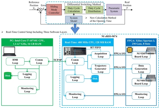
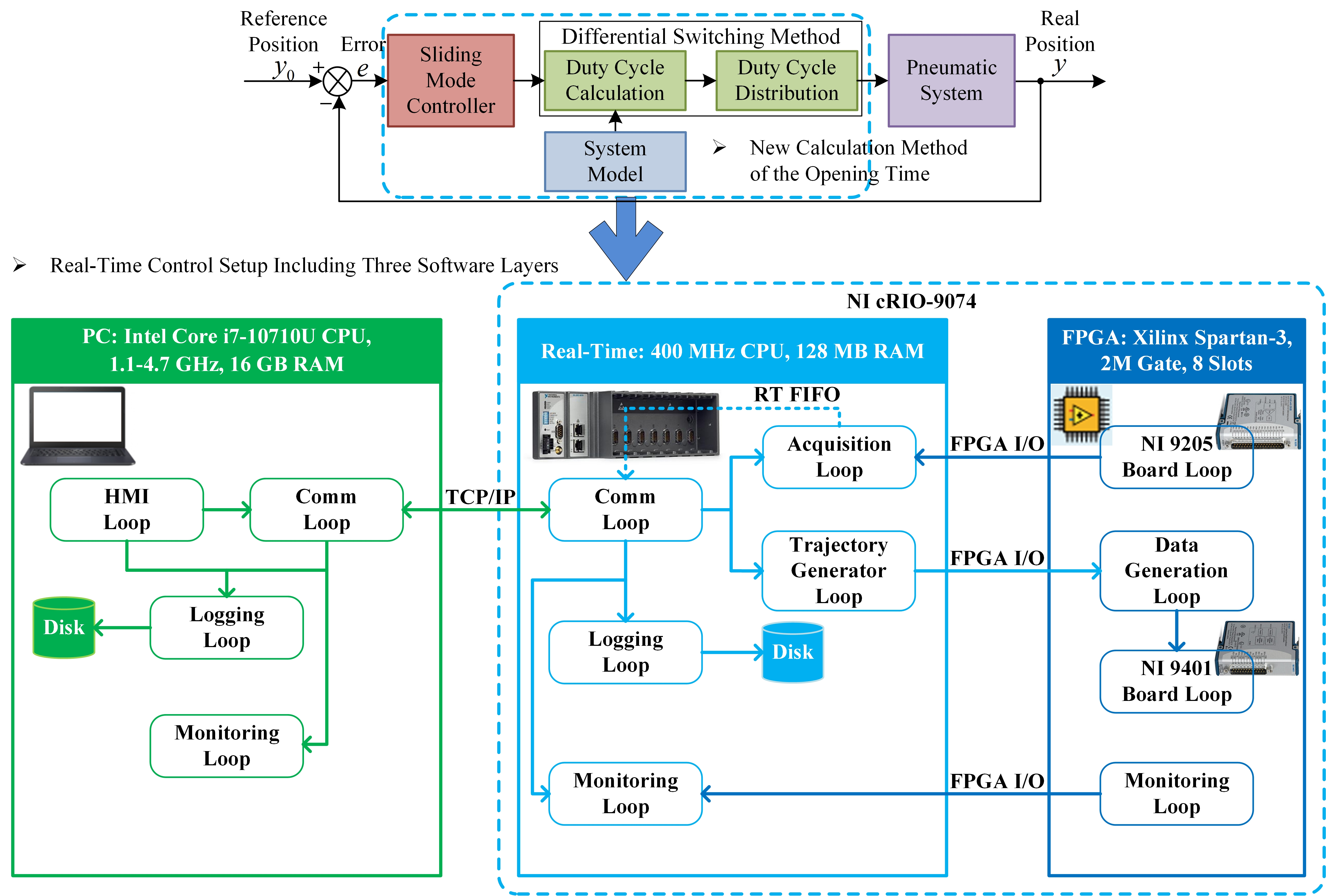
3.1. Differential Switching Method

In the conventional PWM method, the control pulses are shown in Figure 4a. Valves 1 and 4 are open simultaneously, and the control effect is rapidly charging chamber 1 and discharging chamber 2. In this state, the piston will move forward quickly. The duration of the control pulse is $T_d$, PWM period is $T_t$, and the PWM duty cycle is $D=T_d/T_t$. Similarly, valves 2 and 3 are open if the piston needs to move backward. The pulse form of the traditional PWM method is relatively simple, and there are only these two types.

The basic pulse form of the differential switching method is also shown in Figure 4b. In this method, the flow difference generated by the charging and discharging valve of the single-sided chamber is used to create the pressure difference. The control pulses for valves 1 and 2 are started simultaneously. After the synchronized opening time $T_s$ valve 2 is closed, while valve 1 is still open. The differential opening time for valves 1 and 2 is $T_r$. The differential opening time will increase the pressure of chamber 1. For valves 3 and 4, a feasible strategy is to close them all. Under such a control pulse, as the pressure in chamber 1 increases, the piston will move forward, and the volume of chamber 2 decreases. So the pressure in chamber 2 also increases, which is not good for controlling the piston. For this reason, this article innovatively designs the control pulses for valves 3 and 4 to be fully open. From multiple test results, if a pair of charging and discharging valves connected to a chamber with a fixed volume are simultaneously open, the pressure of the chamber will quickly approach a stable value $P_b$. Similarly, simultaneous opening of valves 3 and 4 will cause the pressure in chamber 2 to be close to the stable value.

Table 2. Switching modes of four valves.

	Forward	Stop	Backward
Valve 1	$T_s+T_r$	0	$T_t$
Valve 2	$T_s$	0	$T_t$
Valve 3	$T_t$	0	$T_s+T_r$
Valve 4	$T_t$	0	$T_s$

lists the major switching modes of the differential switching method. For four valves, there are many other possible combinations. For example, valve 2 can be open longer than valve 1, and the effect of this state is similar to the third column of the table. Valve 4 can be open longer than valve 3, and the effect of this state is similar to the first column of the table. Since the effects of these two combinations are similar to those in the table, they are not adopted.

3.2. Calculation Method of the Opening Time

The synchronized opening time $T_s$ and the differential opening time $T_r$ both need to be calculated reasonably to get the best control effect. Firstly, the half-open and half-closed states of the valve are not allowed, so there are the following inequality relationships:

$$\{\begin{array}{c}{T}_{o1}+T_{o2}\le T_t\\ T_{o1}+T_{o2}\le T_s\le T_t\\ T_{o1}+T_{o2}\le T_r\le T_t-T_{o1}-T_{o2}\end{array}$$

(26)

where $T_{o1}$ and $T_{o2}$ are the minimum opening and closing times of the valve. In the choice of PWM cycle, $T_t$ is selected as 2.5 to 5 times of $T_{o1}+T_{o2}$. Secondly, as the primary function of the synchronized opening time is to stabilize the pressure in the compressed chamber of the cylinder during the piston movement, $T_s$ should be as short as possible and satisfy the above inequality. So, the synchronized opening time can be chosen as:

$$T_s=T_{o1}+T_{o2}$$

(27)

Thirdly, the differential opening time leads to the flow changes in the chambers, which eventually generate the pressure difference. In order to simplify the calculation, it is considered that after the synchronized opening time, the double valves on the compressed side no longer produce a flow difference. When calculating the pressure variation of each PWM cycle, a fixed volume of the chamber is used for calculation. From (20), if the volume is fixed, the derivative of pressure is represented as:

$$\dot{P}=\gamma \frac{RT}{V}\dot{m}$$

(28)

It is assumed that at low pressure this equation can model the behaviour of compressed air [25]. According to the definition of the derivative, the following approximate formula can be obtained:

$$T_r=\frac{\left|\Delta P\right|}{\dot{P}}$$

(29)

where $\left|\Delta P\right|$ is the absolute value of the total pressure variation of each PWM cycle. The empirical formula for the differential opening time of the forward and backward movement is proposed considering (28) and (29):

$$T_r=\{\begin{array}{c}\frac{\left|\Delta P\right|}{\gamma \frac{RT}{V}{\displaystyle {\int }_t^{t+T_r}\dot{m}(P_s,P_1)dt}}\\ \frac{\left|\Delta P\right|}{\gamma \frac{RT}{V}{\displaystyle {\int }_t^{t+T_r}\dot{m}(P_s,P_2)dt}}\end{array}$$

(30)

3.3. Sliding Mode Controller Design

After designing the synchronized and differential opening times, a sliding mode controller which is suitable for nonlinear systems with multi switching modes is designed to apply the proposed differential switching method. The displacement error of the cylinder piston is stated as:

$$e=y_0-y$$

(31)

where $y_0$ is the desired piston displacement, and $y$ is the actual piston displacement measured by the displacement sensor. The sliding function can be designed considering the nonlinear system as a second-order system:

$$s=\dot{e}+\sigma e$$

(32)

where $\sigma >0$. The exponential approach law [14] is applied here to guarantee the dynamic quality of approaching movements:

$$\dot{s}=-\epsilon \mathrm{sgn}s-ks$$

(33)

where $\epsilon >0$ and $k>0$ are the exponential approaching parameters. By taking the derivative of (32), $\dot{s}$ can also be stated as:

$$\dot{s}=\ddot{e}+\sigma \dot{e}$$

(34)

where $\dot{e}={\dot{y}}_0-\dot{y}$ and $\ddot{e}={\ddot{y}}_0-\ddot{y}$. By substituting (34) into (33), we can get:

$$\ddot{y}={\ddot{y}}_0+\sigma \dot{e}+\epsilon \mathrm{sgn}s+ks=W(y)$$

(35)

It can be assumed that during the period of charging chamber 1 the pressure change of chamber 2 is negligible due to that the double valves of chamber 2 are open at the same time. The system dynamics of this condition can be achieved as:

$$\ddot{y}=\frac{-B_p}{m_p}\dot{y}+\frac{A_1}{m_p}{P}_1-\frac{A_2}{m_p}{P}_2+\frac{A_1}{m_p}\Delta P$$

(36)

The same can be obtained that:

$$\ddot{y}=\frac{-B_p}{m_p}\dot{y}+\frac{A_1}{m_p}{P}_1-\frac{A_2}{m_p}{P}_2-\frac{A_2}{m_p}\Delta P$$

(37)

The total pressure variation of each PWM cycle $\Delta P$ is set as the output $u$ of the controller. The sliding mode control output is achieved by simplifying the system into three corresponding modes in Table 2: forward, stop, and backward. So, (36) and (37) can also be stated as:

$$\ddot{y}=\{\begin{array}{l}\Gamma +g_{1}u,u>0\\ \Gamma ,u=0\\ \Gamma +g_{2}u,u<0\end{array}$$

(38)

$$\Gamma =\frac{-B_p}{m_p}\dot{y}+\frac{A_1}{m_p}{P}_1-\frac{A_2}{m_p}{P}_2$$

(39)

where $g_1=A_1/m_p$, $g_2=A_2/m_p$. $A_1$, $A_2$, and $m_p$ are all non-negative. The output of the controller can also be achieved by substituting (35) into (38):

$$u_{eq}^{+/-}=\frac{W\left(y\right)-\Gamma }{g^{+/-}}$$

(40)

where

$$g^{+/-}=\{\begin{array}{l}{g}_1,u\ge 0\\ g_2,u<0\end{array}$$

(41)

If the sliding function is positive, the piston will move forward, and $u$ is non-negative. If the sliding function is negative, the piston will move backward, and $u$ is negative.

The Lyapunov-like function is defined as:

$$V=\frac{1}{2}{s}^2$$

(42)

and

$$\dot{V}=s\dot{s}$$

(43)

Considering (32) and (33), $\dot{V}$ can also be achieved as:

$$\dot{V}\le -\epsilon \left|s\right|-k{s}^2=-\frac{k}{2}V-\epsilon \left|s\right|\le -\frac{k}{2}V$$

(44)

From lemma [27,28], if $V:[0,\infty )\in R$, the solution of $\dot{V}\le -\theta V+f$, $\forall t\ge t_0\ge 0$ is

$$V(t)\le e^{-\theta (t-t_0)}V(t_0)+{\displaystyle {\int }_{t_0}^t{e}^{-\theta (t-\tau )}f(\tau )d\tau }$$

(45)

Proof of the lemma: if $\omega (t)\triangleq \dot{V}+\theta V-f$, then $\omega (t)\le 0$. $\dot{V}=-\theta V+f+\omega$ can be solved as:

$$V(t)=e^{-\theta (t-t_0)}V(t_0)+{\displaystyle {\int }_{t_0}^t{e}^{-\theta (t-\tau )}f(\tau )}d\tau +{\displaystyle {\int }_{t_0}^t{e}^{-\theta (t-\tau )}\omega (\tau )}d\tau$$

(46)

As $\omega (t)<0$ and $\forall t\ge t_0\ge 0$, then

$$V(t)\le e^{-\theta (t-t_0)}V(t_0)+{\displaystyle {\int }_{t_0}^t{e}^{-\theta (t-\tau )}f(\tau )d\tau }$$

(47)

If $f=0$, the solution of $\dot{V}\le -\theta V$ is

$$V(t)\le e^{-\theta (t-t_0)}V(t_0)$$

(48)

$V(t)$ will converge to 0 in exponential form if $\theta$ is positive. If the parameters are $\theta =k/2$ and $f=0$, then (44) can be described as:

$$V(t)\le e^{-\frac{k}{2}(t-t_0)}V(t_0)$$

(49)

$V(t)$ can converge to 0 in exponential form. By applying the exponential approach law, the sliding surface $s=0$ can be reached within limited time. The exponential approaching parameter $\epsilon$ is used for adjusting the converging speed while the system is near $s=0$. Another parameter $k$ is used for changing the converging rate while the absolute value of $s$ is large.

The proposed control system block diagram is shown in Figure 5. The system error $e$ is the input of the sliding mode controller, and the controller output is $\Delta P$. The duty cycle is calculated with $\Delta P$ and system model. Then the duty cycle corresponding to the four valves will be logically allocated. The pressure difference produced by the four valves eventually causes the piston to move.

3.4. Parameters Selection and Simulation Results

Two typical simulations are carried out to test the control performance of the proposed method. The proposed sliding mode controller with differential switching method is written as S-function and linked to the system model mentioned above in MATLAB/Simulink. The first contrast simulation is against the traditional PID controller which is described as:

$$u_{pid}=k_{p}e+k_i{\displaystyle {\int }_0^{t}edt+k_d}\dot{e}$$

(50)

where $u_{pid}$ is the PID control output, $k_p$, $k_i$, and $k_d$ are the proportional, integral, and derivative parameters. The PID control output is used for deciding the duty cycle of the conventional PWM method in Figure 4a. In detail, for forward movement valves 1 and 4 are open at the same time. For backward movement valves 2 and 3 are open simultaneously. All valves are closed if the error is small enough. The total mass of the piston and payloads is 1.2 kg. As shown in Figure 6a, the control performance for the proposed method is relatively smooth, and no overshoots or chattering phenomena are observed. For the proposed method, the rising time of the step response is 0.175 s. The PWM period $T_t$ is set to 20 ms, and the synchronized opening time $T_s$ is set to 7 ms due to the standard solenoid on–off valve with 24 V/DC control has a response time of 5 ms in opening and 2 ms in closing. The parameters for the sliding mode controller are chosen as $\sigma =80$, $\epsilon =5$, and $k=50$.

In (32), $\sigma$ is the weighting factor of the error, and $\sigma =80$ means that the weight of the error is 80 times the derivative of the error in the sliding function. This is because the error is usually much smaller than the derivative of the error, and its proportion in the sliding function needs to be increased. $\epsilon$ and $k$ are decided by trial and error. Another critical parameter is the absolute minimum error $e_{\min }$. We set the minimum error range in the simulation program so that all the valves will rapidly stop actuating while the position signal is in this range. $e_{\min }=0.001$ is chosen here to ensure the control accuracy.

A significant overshoot is observed for the PID controller with the conventional PWM method. It takes nearly 0.17 s for the position signal to be stable in the step response. The settling time for both methods is very close. However, the PID controller has some overshoots, and the control effect is worse. Another problem with the PID controller is that the parameters are difficult to estimate accurately. $T_t=20$, $k_p=0.18$, $k_i=0.015$, and $k_d=0.002$ are chosen for the PID controller. It takes much time to adjust these parameters and finally achieved the effect shown in Figure 6a. From the comparison of the two curves, the main reason for the overshoot under the control of PID controller is that when the PID controller outputs a tiny control quantity, the restriction of the minimum opening time of the on–off valve results in a small PID control quantity that cannot be equated to a very small flow rate, resulting in an overshoot in the end.

In the second simulation, the proposed algorithm is used for tracking a sinusoidal signal with a frequency of 0.2 Hz. The simulation results are shown in Figure 7. During the tracking process ranging from −0.03 m to 0.03 m, the maximum error is only 2.54 mm, and the average error is 0.97 mm. Due to the frequency of the sinusoidal signal, it is necessary to appropriately adjust the sliding function parameter $\sigma$ to 150 to improve the response speed of the system. Under the action of the proposed control algorithm, the position signal can quickly follow the given signal.

4. Experimental Setup

The control system setup is shown in Figure 8. In order to ensure the real-time performance of the model calculation, the National Instruments Real-Time (NI RT) platform is selected for real-time model calculation, and an FPGA platform is used for high-precision valve control signal output.

4.1. Pneumatic and Mechanical Setup

The detailed models of the pneumatic and mechanical setup are listed below:

1.

Air supplier. An Outstanding (model 2200X4-160L) air compressor generates the compressed air. A 160 L high-pressure gas tank is integrated with the compressor. This compressor can provide the maximum pressure of 1.2 × 10⁶ Pa. In order to reduce the moisture condensation, a set of filter, regulator, and lubricator (FRL) is set up between the air compressor and the valves;

2.

Pneumatic control components. Four Matrix (model MX 821.103C2XX) 2/2 on–off valves are installed to control the cylinder. This kind of valve can be equipped with the officially designed acceleration circuits (model HSDB 990.012), and its price (about 229 USD) is about four times that of the valve (about 54 USD) itself. Without using the acceleration circuits, the valve opening time is about 5 ms and the closing time is about 2 ms. The valves will have a response time of 1 ms in opening and 1 ms in closing after using the acceleration circuits. The goal of the article is to achieve the best control effect with minimizing costs, so the acceleration circuits are not adopted;

3.

Pneumatic actuator. An Airpel double-acting single-rod cylinder (model M24D100U) is used as the actuator. The cylinder consists of a graphite piston and a borosilicate glass shell has extremely low friction. The stroke of the cylinder is 100 mm, bore diameter is 24 mm, and the rod diameter is 6.35 mm. It can bear the pressure up to 7 × 10⁵ Pa. It has the disadvantage of large air leakage across the piston which wastes energy.

4.

Mechanical setup. The piston rod of the cylinder is connected to a customized payload platform used for carrying the payloads. A payload holding rod is placed in the center of the payload platform to hold the payloads. The payload platform is installed on a HIWIN (model MGW12C) sliding table and a HIWIN (model MGW12C300C) sliding guide. The length of the sliding guide is 300 mm.

4.2. Electrical Setup

The detailed models of the electrical components are listed below.

1.

Industrial Controller. An NI CompactRIO (cRIO) (model 9074) is set as the major controller. NI cRIO is a reconfigurable embedded measurement and control system. It has a robust hardware architecture, including Input/Output (I/O) boards, a chassis with a reconfigurable FPGA, and a real-time controller. The used model 9074 is a low-cost model with eight-slot chassis. A personal computer (PC) is connected to the cRIO via ethernet;

2.

I/O boards. An NI digital I/O board (model 9401) and an analog input board (model 9205) are selected to generate the 5V/TTL signals for the valves and acquire the signals from the sensors. The acquisition configuration for NI 9205 is differential input mode, and the resolution is 16 bit. The nominal input ranges are ±10 V, ±5 V, ±1 V, and ±0.2 V;

3.

Sensors. Three MEACON (model MIK-P300) pressure sensors are used for acquiring the pressures of air supply, chamber 1, and chamber 2. A MIRAN (model KTC-100) position transmitter is set to measure the position of the piston. The resolutions for the used sensors are both customized to 0.02 × 10⁵ Pa and 1 × 10⁻⁵ m, respectively. The output voltage range for the sensors are both 0 V to 5 V. The effective measurement range for MIK-P300 is 0 Pa to 1 × 10⁶ Pa and for KTC-100 is 50 mm to 150 mm;

4.

Power supply and other circuits. A DC power supply is used for powering the entire system. Power and sensor circuits are designed to connect various electronic components. A SANWO DC SSR (model KYOTTO KF0604D) is installed to drive the on–off valves. No acceleration circuits are used for the valves.

4.3. Software Platform and Real-Time Control Setup

In order to achieve the best effect of real-time control, the program is divided into three layers, namely monitoring, calculation, and I/O. Since LabVIEW is a programming language that regards the data flow as its core, the program of each module is represented by loop in Figure 8.

1.

Monitoring layer on PC. Since Microsoft Windows is not a real-time operating system, the LabVIEW programs running on PC cannot achieve precise timing. Therefore, the program on the PC is only for monitoring. The monitoring part is the top level of the software system, consisting of the human machine interface (HMI) loop, communication (comm) loop, logging loop, and monitoring loop. The HMI loop is only responsible for the input and output of the user, and the cycle time for the loop is 100 ms. The comm loop carries out data exchange with cRIO through Transmission Control Protocol/Internet Protocol (TCP/IP), and the cycle time can be set to the fastest to ensure real-time data transmission. The logging loop saves the data to the hard disk. Only some user operation data is saved, and sensor data is not saved here. The monitoring loop displays the data on the screen, and the cycle time can be set to 200 ms. The programming environment on PC is NI LabVIEW Professional Development System 11.0;

2.

Calculation layer on NI RT. By downloading the program into NI RT which is a real-time operating system in Linux, the real-time performance of the program can be guaranteed. The calculation part is the middle level of the software system, consisting of the comm loop, trajectory generator loop, acquisition loop, logging loop, and monitoring loop. The comm loop is used to send data to PC or receive data from PC corresponding to the comm loop on PC, and the cycle time for the loop is set to the fastest. The trajectory generator loop includes the calculation of the algorithm and the model. This part is set to 20 ms. The setting of cycle time balances the computing consumption and real-time requirements. The acquisition loop is set separately. After receiving the command from the comm loop, this loop will use the RT First Input First Output (FIFO) for data collection. The RT FIFO function is used to send and receive data in a deterministic manner between VIs which represent subprograms in LabVIEW. The deterministic data transfer of the RT FIFO function does not add jitter to the cycle time of the loop. The cycle time of this loop is set to 1 ms. The logging loop will record all the acquiring data to the hard disk on cRIO, and its cycle time is 1 ms, too. The monitoring loop is the display output of the cRIO itself. Since it does not need to be used, it is disabled here. The programming environment on NI RT is NI LabVIEW Real-Time Module 11.0;

3.

I/O layer on FPGA. Using FPGA as the bottom layer of the program further ensures real-time performance. I/O part consists of the NI 9205 board loop, data generation loop, NI 9401 board loop, and monitoring loop. Among them, the NI 9205 board loop is responsible for collecting the data, directly using FPGA I/O to transmit the data to the acquisition loop on NI RT. The signal generates by the NI 9401 board is from the data generation loop which works with the trajectory generator loop on NI RT. The programming environment on FPGA is NI LabVIEW FPGA Module 11.0.

Through the above-mentioned three-layer program setting, the real-time signal acquisition and output are ensured.

4.4. Overall Setup

Figure 9 shows the actual system which is connected based on Figure 8. A PC is connected to the NI cRIO through ethernet. The digital output board on the cRIO controls the on–off valves via DC SSR. The sensor signals are acquired by the analog input board with the sensor circuits. The air compressor provides the air supply for the control system, and the piston rod of the cylinder will move under the action of the valves.

5. Experimental Results and Discussion

The experimental verification is divided into three parts. In the first part, the proposed sliding mode controller with differential switching method (SMC+DS) is compared to three other controllers: the PID controller with differential switching method (PID+DS), the PID controller with PWM method (PID+PWM), and the seven-mode model based controller from S. Hodgson et al. (MBC7) [18]. In the second part, two experiments will show the dynamic performance of the proposed controller. In the last part, a step response tracking test will show the control performance under different payloads.

5.1. Comparative Experiments between Four Controllers

In the contrast experiment, four controllers (SMC+DS, PID+DS, PID+PWM, and SMC7) are applied. The purpose of setting up the above four controllers is: (a) The control effect of SMC+DS can be compared to that of PID+DS. It will show the advantage of SMC over PID. (b) The control effect of PID+DS can be compared to that of PID+PWM. It can show the advantage of DS over PWM. (c) The control effect of SMC+DS can be compared to that of PID+PWM and MBC7. PID+PWM is the traditional method for pneumatic position control, and MBC7 is the state-of-the-art controller in this field [18]. The superiority of the proposed method can be demonstrated by the comparison. Figure 10 shows the experimental results for the four controllers. Total payloads for the test are 1.2 kg (0.2 kg for the piston and 1 kg for the payloads).

Through 20 tests, the average rinsing time, overshoot, and steady-state error are summarized in

Table 3. Main control performance comparison between the four controllers.

	SMC+DS	PID+DS	PID+PWM	MBC7
Rising time (average)	0.31 s	0.35 s	0.36 s	0.33 s
Overshoot (average)	0.83%	3.33%	5.57%	2.93%
Steady-state error (average)	0.18 mm	0.25 mm	0.28 mm	0.21 mm

. For the proposed method, the parameters selected in the experiment are $T_t=20$, $T_s=7$, $\sigma =35$, $\epsilon =5$, $k=50$, and $e_{\min }=0.001$. Then in the PID controller, parameters are $T_t=20$, $k_p=0.22$, $k_i=0.025$, and $k_d=0.001$. PID parameters are chosen by multiple tests and experience. The control effect is clear that SMC+DS is better than PID+DS. Since they both based on the differential switching method, the control curves are very similar. However, since PID is not a nonlinear controller, its control effect is not as good as SMC.

Since the proposed differential switching method in this paper and PWM method are both modulation method for on–off valve, they cannot be used and tested alone. So here PID is applied as the system controller to compare their output differences. The PID parameters are same in PID+DS and PID+PWM. In the experimental results, they both show some overshoots and steady-state errors. Rising time (average) for PID+DS is 0.35 s and for PID+PWM is 0.36 s. Steady-state error (average) for PID+DS is 0.25 mm and for PID+PWM is 0.28 mm. The PID-DS method mainly has a large advantage in average overshoot, reducing that from 5.57% to 3.33%. The cause of the overshoots is consistent with the simulation part. The minimal PID control output cannot be accurately converted into tiny flow changes. The restriction of the minimum valve opening time results in an inaccurate flow output. In the actual test, there may be multiple overshoots and oscillations. The differential switching method can produce more accurate output control in the low error segment because it takes into account the dead zone of the on–off valve.

Then the proposed method is compared to PID+PWM and MBC7 method. MBC7 is a seven-mode model based controller from S. Hodgson et al. [18] which is an improved switched controller with seven modes (SC7) [17]. The original MBC7 is applied with on–off valves using acceleration circuits. The control effect of removing the acceleration circuits is not clear. MBC7 is applied without the use of acceleration circuits in this study, so the experimental results may be different from the original research. Most parameters of MBC7 are consistent with the original research and the sliding mode parameters are set as consistently as possible with the SMC we use. From Figure 10 and Table 3, the proposed method achieves the lowest average rising time (0.31 s), overshoot (0.83%), and steady-state error (0.18 mm), nearly no overshoots, and no oscillations. For MBC7, the average rising time (0.33 s) and steady-state error (0.21 mm) are very close to SMC+DS. However, the average overshoot (2.93%) is larger than the proposed method. Comparing Figure 10c–f, more switching times are required for the proposed method, which is an unavoidable defect of the method. The proposed method requires more switching of the four valves to achieve high-precision flow control. Taken together, the method proposed in this paper is superior to MBC7 and PID+PWM.

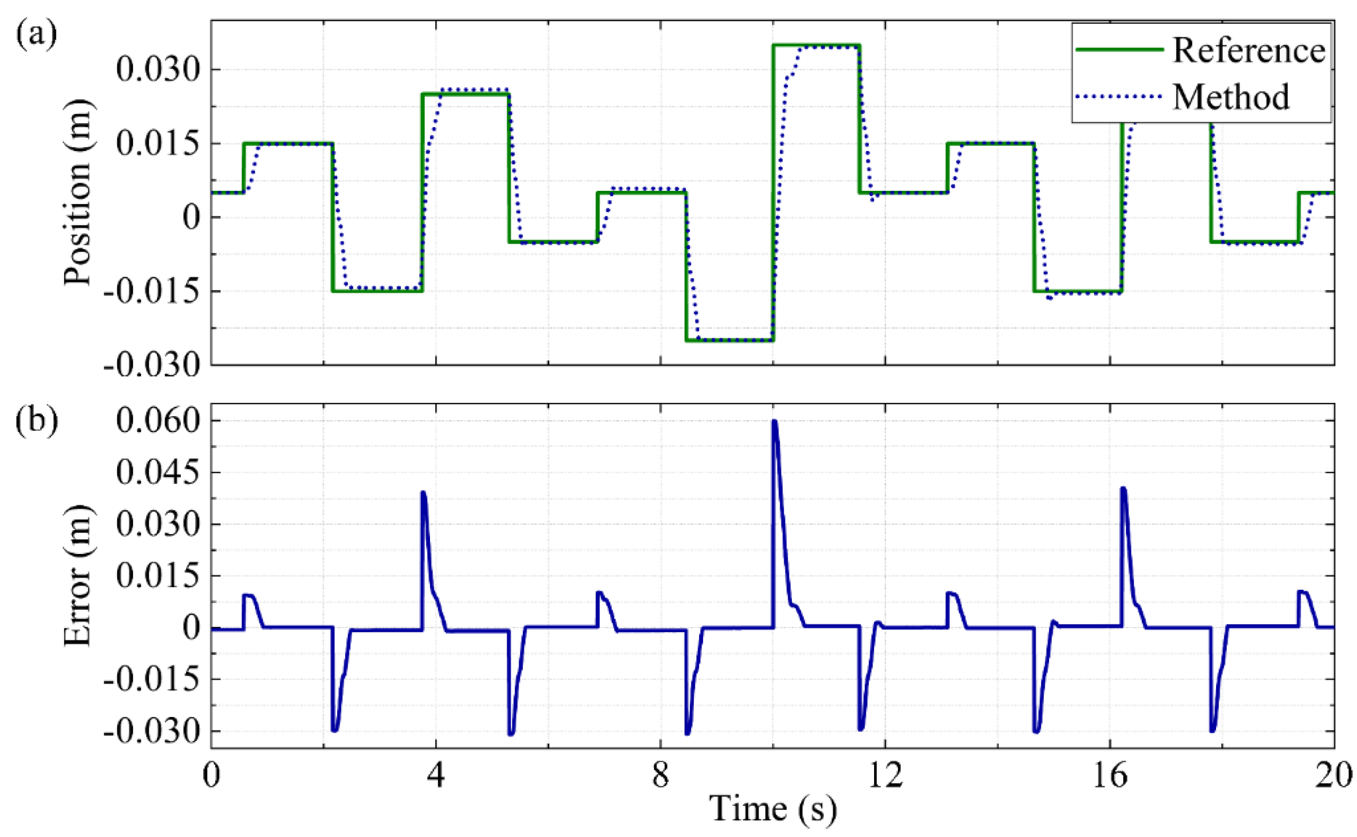
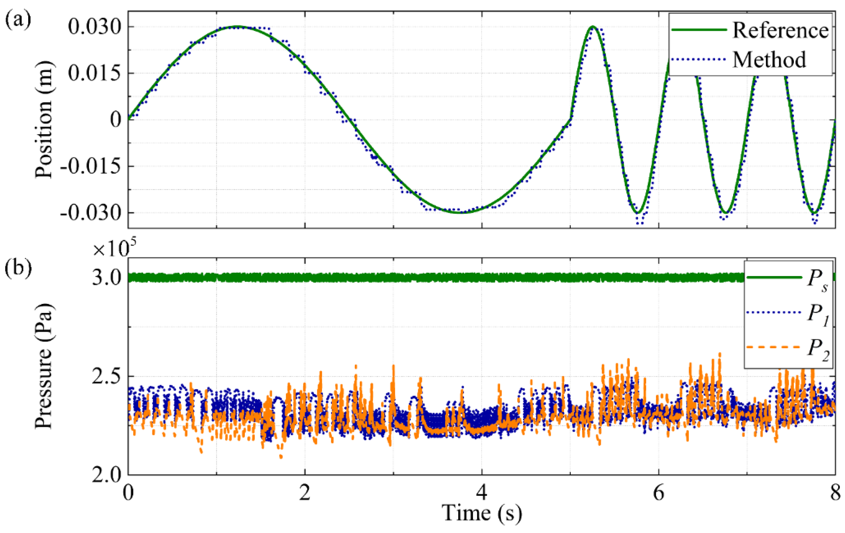
5.2. Dynamic Response Experiments

A random step response test is carried out to show the continuous position tracking performance. In order to achieve a faster continuous response, the parameters have been adjusted. $\sigma =28$, $\epsilon =4.5$, $k=55$, and $e_{\min }=0.002$ are the selected parameters. While tracking the step response ranging from −0.025 m to 0.035 m in Figure 11, the proposed method achieves rising time between 0.28 s to 0.44 s, overshoot between 1.13% to 4.67%, and steady-state error between 0.2 mm to 0.9 mm. It can be seen that compared to the first experiment, the rise time has been reduced, but overshoot has occurred, and the steady-state error has also increased. In terms of tracking performance, it can quickly respond to the given step signal.

Then, the given signal is changed into a sinusoidal signal with variable frequency. The former wave has a frequency of 0.2 Hz and the latter wave has a frequency of 1 Hz. For a chamber with a fixed volume, if the charging valve and discharging valve connected to it are continuously open, and the air supply pressure is 3 × 105 Pa, the final pressure will stabilize to $P_b=2.431\times {10}^5\mathrm{Pa}$. As shown in Figure 12b, most of the pressure also fluctuates around this value. This is because the proposed method requires a synchronized opening time for the four valves, which makes them open simultaneously. During this time, the pressure will be close to this value. From the tracking effect of Figure 12a, the response signal can closely follow the given signal, and no delay occurs. The average error is about 1.68 mm. The parameters of this experiment are consistent with the second experiment.

5.3. Step Response Experiments under Different Payloads

As shown in Figure 13, the control effects under the condition of changing payloads are compared. The rising time in the increasing period of the step response is 0.42 s, 0.69 s, and 1.1 s for 1.25 kg, 3.25 kg, and 5.25 kg. The rising time in the decreasing period of the step response is 0.43 s, 0.51 s, and 0.69 s for 1.25 kg, 3.25 kg, and 5.25 kg. No overshoots are observed in the experiment. The biggest steady-state error is about 0.5 mm for all conditions. This result shows that the proposed method can also achieve high-precision positions under variable payload conditions.

The experimental results indicate that the sliding mode controller with differential switching method is effective in the position tracking system. Two main innovations ensure high-performance position tracking:

1.

Differential switching method. In the proposed method, the flow difference generated by the charging and discharging valve of the single-sided chamber is used to create the pressure difference. The opening time of the four valves is strictly regulated, and calculation method of the opening time are given. The innovative method can replace the traditional PWM method and be applied with the nonlinear controller.

2.

Real-time control setup. The control program is reasonably divided into three layers including monitoring layer on PC, calculation layer on NI RT, and I/O layer on FPGA. Suggested values of the cycle time for all programs are given. Assigning different cycle time to different tasks and using RT FIFO for important tasks ensure the timely response of each program and the real-time of the overall program.

Overall, the experimental results demonstrate that the method of differential switching method instead of the conventional PWM method is feasible in the pneumatic positioning system with low-cost on–off valves.

6. Conclusions

In the pneumatic positioning system of the industrial automated production line, a differential switching method is proposed to control a pneumatic cylinder with four low-cost on–off valves. The purpose of the new method is to achieve the best performance without using the acceleration circuits for the on–off valves to lower the costs of the whole system. The proposed method is applied instead of the conventional PWM method, and the calculation method of the opening time is given. The real-time control setup, including three software layers, is proposed to implement the algorithm. Then, the differential switching method is combined with the sliding mode controller, and the system stability is proved. Two simulations and four experiments are carried out to test the control performance of the proposed method. The proposed method shows better results in the contrast experiment than the PID controller with differential switching method, the PID controller with PWM method, and the seven-mode model based controller from S. Hodgson et al. The proposed method achieves the lowest average rising time (0.31 s), overshoot (0.83%), and steady-state error (0.18 mm), nearly no overshoots, and no oscillations. In the experiments of tracking the random step and sinusoidal response, the tracking performance is good enough, and no delay occurs. While tracking the sine wave, the maximum frequency is 1 Hz, and the average error is 1.68 mm. In the variable payload test, it can still have a better control effect under the maximum load of 5.25 kg. Only 0.5 mm steady-state error is observed. All simulation and experimental results show that the proposed method can ensure the control effect only using the traditional on–off valve without the acceleration circuits.

1.

The main limitations of the research and the future work are summarized as: The embedded control system used in this research is NI cRIO-9074. It is an expensive platform, and the price of the total platform and digital boards is about 4500 USD. Compared with other components in the system, the price of the platform can be further reduced, such as using some commercial products or developing an embedded system ourselves. To reduce the costs, MangoTree AtomRIO controller which is based on Intel Core CPU and Xilinx Spartan-LX75 FPGA is recommended for this system. The price of this plan is about 1200 USD. Since the real-time operating system (RTOS) and FPGA are needed, it is recommended to use ARM (Advanced RISC Machine) and FPGA design on the hardware architecture. A typical design is to used XILINX Zynq-7000 SoC (System on Chip). The hardware design and production costs will be reduced to about 1000 USD. So, the next step for the research is to design an embedded control system based on Zynq-7000 SoC to further reduce the costs.

2.

The proposed control method is extremely dependent on the accuracy of the system model. If it needs to be used in the real engineering project, it is necessary to solve the problem that the parameters of the real system model are difficult to determine. Therefore, in the next step, we will explore how to use field-collected data for modeling, such as neural networks or deep learning methods, to ensure the performance of the controller.

3.

In this research, the error value is just subtracting from the analog-to-digital converter (ADC) reading and then getting a mean value. A better way to perform the measurements is through a specialized device which is calibrated. A dial indicator is usually used in this task with adequate resolution and range. In the next step, we will carry out these measurements with a dial indicator and then trace the error curve where the error behaviour over the measurement range can be seen.

References

1. Hadi, H.H.; Sallom, M.Y. Pneumatic Control System of Automatic Production Line Using SCADA Implement PLC. In Proceedings of the 2019 4th Scientific International Conference Najaf (SICN), Al-Najef, Iraq, 29–30 April 2019; pp. 37–42. [Google Scholar] [CrossRef]
2. Zhou, Y.; Li, Y. PLC Control System of Pneumatic Manipulator Automatic Assembly Line Based on Cloud Computing Platform. J. Phys. Conf. Ser. 2021, 1744, 022011. [Google Scholar] [CrossRef]
3. Zhao, S.; Li, D.; Zhou, J.; Sha, E. Numerical and Experimental Study of a Flexible Trailing Edge Driving by Pneumatic Muscle Actuators. Actuators 2021, 10, 142. [Google Scholar] [CrossRef]
4. Cantoni, C.; Gobbi, M.; Mastinu, G.; Meschini, A. Brake and pneumatic wheel performance assessment—A new test rig. Measurement 2019, 150, 107042. [Google Scholar] [CrossRef]
5. Lu, S.; Chen, D.; Hao, R.; Luo, S.; Wang, M. Design, fabrication and characterization of soft sensors through EGaIn for soft pneumatic actuators. Measurement 2020, 164, 107996. [Google Scholar] [CrossRef]
6. Belforte, G.; Mauro, S.; Mattiazzo, G. A method for increasing the dynamic performance of pneumatic servosystems with digital valves. Mechatronics 2004, 14, 1105–1120. [Google Scholar] [CrossRef]
7. Carneiro, J.F.; De Almeida, F.G. Accurate motion control of a servopneumatic system using integral sliding mode control. Int. J. Adv. Manuf. Technol. 2014, 77, 1533–1548. [Google Scholar] [CrossRef]
8. Taghizadeh, M.; Najafi, F.; Ghaffari, A. Multimodel PD-control of a pneumatic actuator under variable loads. Int. J. Adv. Manuf. Technol. 2009, 48, 655–662. [Google Scholar] [CrossRef]
9. Systems, Solutions and Expertise for the Automotive and Tier 1 Supplier Industry. Available online: https://www.festo.com/net/SupportPortal/Files/467715/PO-for-the-automotive-Tier1-supplier-industry_EN_2016-07c.pdf (accessed on 1 July 2016).
10. Noritsugu, T. Development of PWM mode electro-pneumatic servomechanism. I: Speed control of a pneumatic cylinder. J. Fluid Control 1986, 17, 65–80. [Google Scholar]
11. Zhang, J.; Lv, C.; Yue, X.; Li, Y.; Yuan, Y. Study on a linear relationship between limited pressure difference and coil current of on/off valve and its influential factors. ISA Trans. 2013, 53, 150–161. [Google Scholar] [CrossRef] [PubMed]
12. Van Varseveld, R.; Bone, G. Accurate position control of a pneumatic actuator using on/off solenoid valves. IEEE/ASME Trans. Mechatron. 1997, 2, 195–204. [Google Scholar] [CrossRef]
13. Ming-Chang, S.; Ming-An, M. Position Control of a Pneumatic Rodless Cylinder Using Sliding Mode M-D-PWM Control the High Speed Solenoid Valves. JSME Int. J. Ser. C 1998, 41, 236–241. [Google Scholar] [CrossRef] [Green Version]
14. Lin, Z.; Zhang, T.; Xie, Q. Intelligent real-time pressure tracking system using a novel hybrid control scheme. Trans. Inst. Meas. Control 2017, 40, 3744–3759. [Google Scholar] [CrossRef]
15. Thanh, T.D.C.; Ahn, K.K. Nonlinear PID control to improve the control performance of 2 axes pneumatic artificial muscle manipulator using neural network. Mechatronics 2006, 16, 577–587. [Google Scholar] [CrossRef]
16. Lin, Z.; Wei, Q.; Ji, R.; Huang, X.; Yuan, Y.; Zhao, Z. An Electro-Pneumatic Force Tracking System using Fuzzy Logic Based Volume Flow Control. Energies 2019, 12, 4011. [Google Scholar] [CrossRef] [Green Version]
17. Hodgson, S.; Le, M.Q.; Tavakoli, M.; Pham, M.T. Improved tracking and switching performance of an electro-pneumatic positioning system. Mechatronics 2012, 22, 1–12. [Google Scholar] [CrossRef] [Green Version]
18. Hodgson, S.; Tavakoli, M.; Pham, M.T.; Lelevé, A. Nonlinear Discontinuous Dynamics Averaging and PWM-Based Sliding Control of Solenoid-Valve Pneumatic Actuators. IEEE/ASME Trans. Mechatron. 2014, 20, 876–888. [Google Scholar] [CrossRef] [Green Version]
19. Nguyen, T.; Leavitt, J.; Jabbari, F.; Bobrow, J.E. Accurate Sliding-Mode Control of Pneumatic Systems Using Low-Cost Solenoid Valves. IEEE/ASME Trans. Mechatron. 2007, 12, 216–219. [Google Scholar] [CrossRef]
20. Lin, C.-J.; Sie, T.-Y.; Chu, W.-L.; Yau, H.-T.; Ding, C.-H. Tracking Control of Pneumatic Artificial Muscle-Activated Robot Arm Based on Sliding-Mode Control. Actuators 2021, 10, 66. [Google Scholar] [CrossRef]
21. dos Santos, M.P.S.; Ferreira, J.A.F. Novel intelligent real-time position tracking system using FPGA and fuzzy logic. ISA Trans. 2014, 53, 402–414. [Google Scholar] [CrossRef]
22. Lin, Z.; Zhang, T.; Xie, Q.; Wei, Q. Electro-pneumatic position tracking control system based on an intelligent phase-change PWM strategy. J. Braz. Soc. Mech. Sci. Eng. 2018, 40, 512. [Google Scholar] [CrossRef]
23. Sakurai, T.; Newton, A. Alpha-power law MOSFET model and its applications to CMOS inverter delay and other formulas. IEEE J. Solid-State Circuits 1990, 25, 584–594. [Google Scholar] [CrossRef] [Green Version]
24. Taghizadeh, M.; Ghaffari, A.; Najafi, F. Modeling and identification of a solenoid valve for PWM control applications. Comptes Rendus Mec. 2009, 337, 131–140. [Google Scholar] [CrossRef]
25. Beater, P. Pneumatic Drives: System Design, Modelling and Control, 1st ed.; Springer: Berlin/Heidelberg, Germany, 2007; pp. 11–39. [Google Scholar] [CrossRef]
26. Richer, E.; Hurmuzlu, Y. A High Performance Pneumatic Force Actuator System: Part I—Nonlinear Mathematical Model. J. Dyn. Syst. Meas. Control. 1999, 122, 416–425. [Google Scholar] [CrossRef]
27. Ioannou, P.; Sun, J. Robust Adaptive Control, 1st ed.; Prentice Hall PTR: Hoboken, NJ, USA, 1996; pp. 75–76. [Google Scholar]
28. Lin, Z.; Zhang, T.; Xie, Q.; Wei, Q. Intelligent Electro-Pneumatic Position Tracking System Using Improved Mode-Switching Sliding Control With Fuzzy Nonlinear Gain. IEEE Access 2018, 6, 34462–34476. [Google Scholar] [CrossRef]
Figure 1. Schematic diagram of the pneumatic positioning system on the production line.
Actuators 10 00260 g001
Figure 2. Block diagram of the major components in the on–off valve and its interaction with the N-MOSFET: (a) N-MOSFET; (b) electromagnetic components; and (c) mechanical components and fluid system.
Actuators 10 00260 g002
Figure 3. Block diagram of the integrated model.
Actuators 10 00260 g003
Figure 4. Two modulation methods: (a) conventional PWM method; and (b) differential switching method (Charge Chamber 1).
Actuators 10 00260 g004
Figure 5. Sliding mode controller with differential switching method.
Actuators 10 00260 g005
Figure 6. Simulation results of the step response for the sliding mode controller with differential switching method and the traditional PID controller: (a) position; and (b) position error.
Actuators 10 00260 g006
Figure 7. Simulation results of the sinusoidal response for the sliding mode controller with differential switching method: (a) position; and (b) position error.
Actuators 10 00260 g007
Figure 8. Overall control system setup with the specific program allocation in PC, NI RT, and NI FPGA.
Actuators 10 00260 g008
Figure 9. Pictures of the real system.
Actuators 10 00260 g009
Figure 10. Experimental results of the step response for the sliding mode controller with differential switching method (SMC+DS), the PID controller with differential switching method (PID+DS), the PID controller with PWM method (PID+PWM), and the seven-mode model based controller from S. Hodgson et al. (MBC7): (a) position; (b) position error; (c) control pulse of the valve 1 from the sliding mode controller with differential switching method; (d) control pulse of the valve 1 from the PID controller with differential switching method; (e) control pulse of the valve 1 from the PID controller with PWM method; and (f) control pulse of the valve 1 from the seven-mode model based controller from S. Hodgson et al.
Actuators 10 00260 g010
Figure 11. Experimental results of the random step response for the sliding mode controller with differential switching method: (a) position; and (b) position error.
Actuators 10 00260 g011
Figure 12. Experimental results of the sinusoidal response for the sliding mode controller with differential switching method: (a) position; and (b) pressure.
Actuators 10 00260 g012
Figure 13. Experimental results of the step response under different payloads for the sliding mode controller with differential switching method: (a) position; and (b) position error.
Actuators 10 00260 g013