Article

Examining Yam Production in Response to Climate Change in Nigeria: A Co-Integration Model Approach

1
School of Agriculture, Food and Environment, Royal Agricultural University, Stroud road, Cirencester GL7 6JS, UK
2
Department of Agricultural Economics, University of Calabar, Etagbor, Calabar PMB 1115, Cross River State, Nigeria
3
School of Business and Entrepreneurship, Royal Agricultural University, Stroud road, Cirencester GL7 6JS, UK
*
Author to whom correspondence should be addressed.
Soc. Sci. 2020, 9(4), 42; https://doi.org/10.3390/socsci9040042
Submission received: 12 March 2020 / Revised: 31 March 2020 / Accepted: 1 April 2020 / Published: 4 April 2020
(This article belongs to the Section Social Economics)

Abstract

:
This study addressed yam production in response to climate change in Cross River State using a co-integration model approach. The specific objectives of this paper are to analyze the trend in yam production, annual precipitation, and annual temperature, and to analyze the impact of climate variables on yam production. Time-series data from 1996 to 2017 was used. Based on the analysis, which constituted a linear trend analysis, co-integration test, and error correction model, the study came up with robust findings. The linear trend analysis for yam production revealed a steady increase in output between the years 2005 and 2016. The result of the rainfall trend analysis showed the presence of rainfall variability and irregularity. The trend line for temperature showed an overall downward trend for the period under study. However, the Error Correction Model result showed that temperature was statistically significant and negatively impacted yam production. The study recommends that policymakers should take appropriate steps to encourage the development of pest- and disease-tolerant yam varieties because an increase in temperature leads to the proliferation of insects, pests, and diseases.

1. Introduction

Agriculture is one of the sectors that are climate-sensitive in Nigeria. This is because agricultural production is mostly rain-fed. Cultivation is mainly dependent on rainfall, and therefore, any change in climate will impact production directly and also affect other socio-economic activities in the country (Egbe et al. 2014; Elijah Samuel et al. 2018). Impacts are measured in terms of the effect on crop growth, availability of soil water, soil erosion, incidence of pest and disease, sea-level rise, and decrease in soil fertility (Dinar et al. 2008; Thomas-Hope 2017), all of which impact the wellbeing of rural communities. Though the threat of a changing climate is universal, agricultural production activities are usually more susceptible than other sectors (Mbanasor et al. 2015).
Consequently, this study seeks to address the impact of climate change on yam production, which is a staple food in Cross River State, Nigeria. According to literature, there have been studies on effects of climate change on agriculture in Nigeria using secondary time series data at state and national level (Agwu et al. 2012; Enete 2014; Akinbobola et al. 2015; Nwaobiala and Nottidge 2015; Mbanasor et al. 2015; Elijah Samuel et al. 2018). Nevertheless, very few of these studies used time-series data to determine the stationarity properties, which is a prerequisite for the estimation of time-series data that is more than 20 years (Sarker et al. 2012; Eregha et al. 2014; Verter and Bečvářová 2015). For this reason, the high R-squared values estimated by these studies may be considered to be a spurious regression resulting in a biased estimate. Additionally, these studies did not address the problem of autocorrelation and heteroscedasticity (Tesso et al. 2012; Sarker et al. 2012; Mbanasor et al. 2015). Moreover, the impact of climate change is crop and location-specific, so it is essential to research a specific crop in a particular location (Sarker et al. 2012). Hence, this research focused on yam crop in Cross River State using time series data.
Subsequently, this present research attempts to fill this gap created in the literature. As a prerequisite for the estimation of time series data, a unit root test was carried out using the Augmented Dickey–Fuller (ADF) test to examine each of the study variables to detect the presence of a unit root (i.e., an indication of stationarity for each variable). This estimate is carried out in this study to ensure that the results obtained are not spurious. However, the overall estimation was in the following order: the unit root test, Johansen’s co-integration test, trace test, the Error Correction Model test, and finally, the post-regression test.
Therefore, the objectives of this study are to analyze the trend in yam production, annual precipitation, and annual temperature, and to investigate the impact of climate variables on yam output.

2. Materials and Methods

2.1. The Study Area

The study was undertaken in Cross River State, Nigeria. Cross River State belongs to the south-south geopolitical zone in Nigeria and is an outstanding food crop-producing state in the country. It is situated between latitudes 5°32′ N and 4°27′ N and longitudes 7°50′ and 9°28′ E. The state lies within the tropics and shares borders with the Cameroon Republic in the East, Benue state in the North, Enugu and Abia States in the West and Akwa-Ibom state in the south. Situated in the Niger Delta region of Nigeria, the state covers an area of 20,156 square kilometers with a population of 3.7 million and a population density of 190 inhabitants per square kilometer (NPC 2011).
Two distinct seasons are experienced in the state: Wet season and dry season. The wet season starts in February/March and continues till October/November, while the dry season begins in November/December and continues till January/February. The mean annual rainfall from 1300 to 3000 mm prevails over the state, and this varies from place to place. The highest temperature is recorded between February and March and does not exceed 37 °C and the lowest between May and October and does not go below 15 °C and also varies from place to place. The vegetation of the state comprises four different features, which range from Mangrove Swamp (wetland), through the rainforest, to derived savannah and finally montane parkland (Angba et al. 2018).
Moreover, the two significant soil types found in the area are the deep laterite fertile soil and dark clayey basalt soil. The weather conditions and the full range of vegetation types give the farmers in Cross River State advantage in the cultivation of oil palm, cocoa, cassava, yams, plantain, rice, maize, sweet potatoes, and a wide range of vegetables including waterleaf, telfera, amaranthus spp, okra, pepper, etc.
Historically, the people of Cross River state have been Christians, and the principal occupation here is farming, trading, and teaching. Cross River State indigenes are also engaged in fishing and poultry farming. The map of the study area is shown in Figure 1.

2.2. Data Collection

Data required for this study was generated from a secondary source. Secondary data on the composition of annual yam output, annual temperature, and annual rainfall were gathered from government statistical bulletin, Central Bank of Nigeria and Nigeria Meteorological Agency between 1996 and 2017 (period under study). There was a challenge in collecting secondary data over a long period in Cross River State. Hence, these were the data available in the state’s database.

2.3. Data Analysis and Model Specification

2.3.1. Production Function Model Specification:

In its most standard form for production of a single commodity that has two factors, the function is specified thus:
Y = f (X1, X2)
where
  • Y = output of yam (kg)
  • f = functional form
  • X1 = rainfall (mm)
  • X2 = temperature (°C)
However, data will be analyzed using the Cobb–Douglas production function and the model is specified thus:
Y = ARa + Tβ
where A, a and β are positive parameters where = a > O, β > O.
The log form is specified as:
Log Y = β0 + β1Log (R) + β2Log (T) + e
where:
  • Y = output of yam (tonnes)
  • R = rainfall (mm)
  • T = temperature (°C)
  • β = coefficients to be estimated
  • e = stochastic variable
Therefore, the statistical tool that will be used to analyze the data collected for yam output, area harvested, rainfall, and temperature, is the multiple regression. This is so because multiple regression allows one to observe the relationship between multiple exogenous variables and a dependent variable. This relationship observed allows the researcher to predict why the outcome is what it is.
The formula for multiple regression is, however, given as:
Y = a + b1X1 + b2X2 + b3X3 + U
where
  • Y = the dependent variable (output of yam)
  • a = intercept of Y (constant)
  • b = slope or coefficient of X
  • X1 = rainfall (in mm)
  • X2 = temperature (in °C)
  • U = error term

2.3.2. Unit Root Test

The first step in the analysis of co-integration is to investigate the stationarity of the time series involved. This step involves testing the order of integration of the individual series under consideration. The augmented Dickey–Fuller test, relies on rejecting a null hypothesis of a unit root (if the series are non-stationary) in favor of the alternative hypothesis.

2.3.3. The Co-Integration Test

In a regression model that involves non-stationary variables, spuriousness can only be avoided by establishing a stable co-integration relationship between the variables. The concept of co-integration states that if there is a long-run relationship between two variables, then the deviation from the long-run equilibrium path should be bounded. If this is the case, then the variables are co-integrated (Sarker et al. 2012).
This study will adopt Engle and Granger two-step procedure approach. According to the procedure, if two or more time-series X1 and Y1 co-integrate, a linear combination of them must be stationary, i.e., Y1 = Ut, where Ut is stationary.

2.3.4. Error Correction Model

If there is a prove that co-integration exists, then the construction of an error correction mechanism to model dynamic relationships will be required, which is the third step. The error correction model aims to show the speed of adjustment from the short-run equilibrium to the long-run equilibrium state. The higher the co-efficient of the parameter, the greater the rate of alteration of the model from the short-run to the long-run.

2.3.5. Multivariate Model Specification

The multivariate regression analysis model is specified thus:
InQ = β0 + β1InX1 + β2InX2 + u
where:
  • β = regression coefficient
  • Q = output of yam
  • X1= mean annual temperature (degree centigrade)
  • X2= mean annual rainfall (millimeter)
  • U = random error term
The co-integration model for the study is specified thus:
Yt = f(X1, X2)
Estimating Equation (1) in an estimate form,
Yt = a0 + a1X1 + a2X2
The model is specified in log-linear form as:
Log (Yt) = a0 + a1 Log X1 + a2 Log X2 + Ut
where:
  • Yt = output of yam
  • X1 = annual temperature (°C)
  • X2 = annual rainfall (mm)
  • Ut = stochastic error term

3. Results and Discussion

3.1. Trend Analysis of Yam Output and Climate Variables

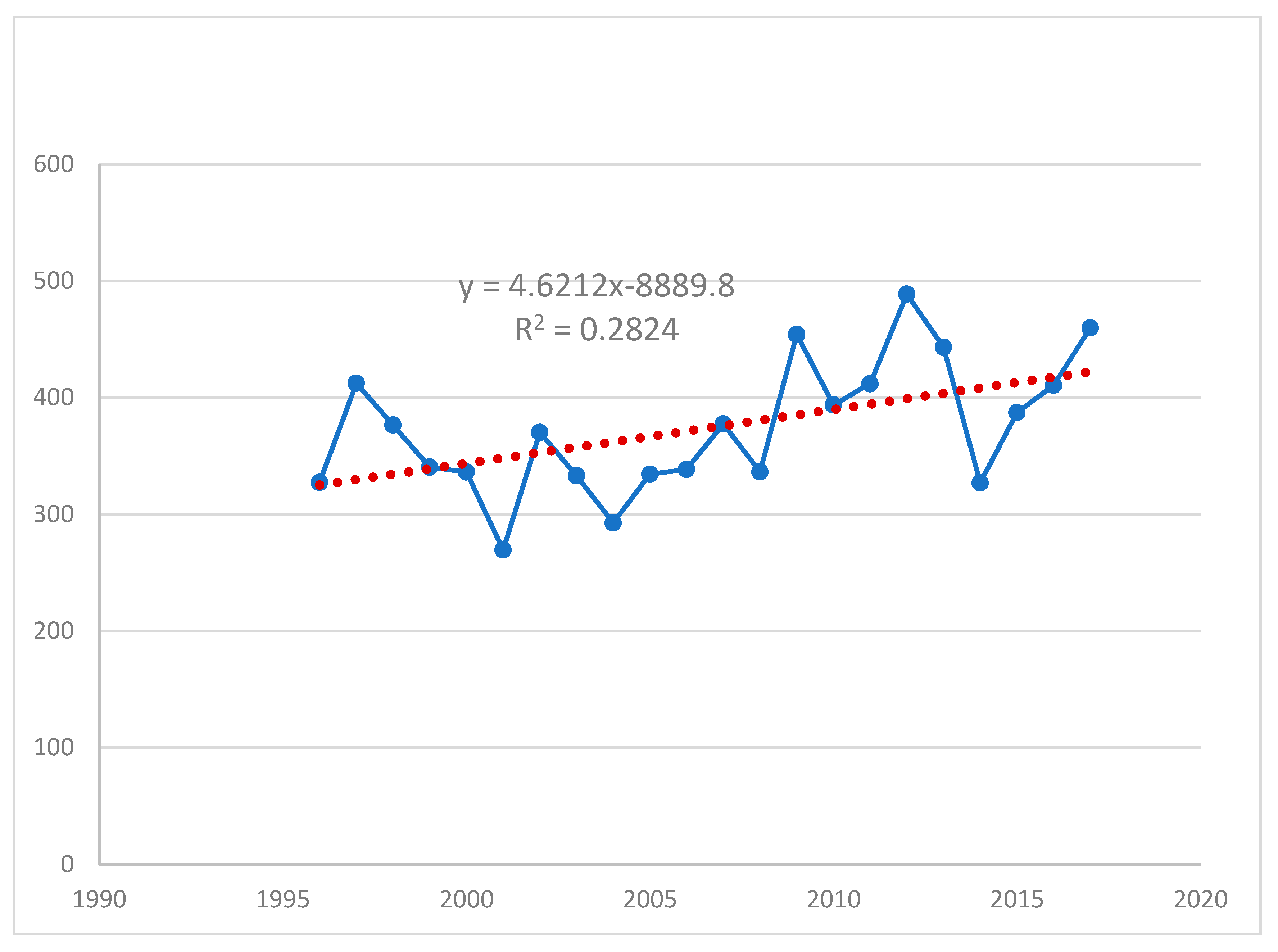
3.1.1. The Trend of Yam Production

Figure 2 below illustrates the trend analysis of yam production for the period under study (1996–2016). The trend analysis shows an upward trend in yam production for the entire period. Nevertheless, low output in yam was observed between 1996 and 2004. This low output of yam found during this time may have been due to the decline in the total labor force in agriculture from 59% in the 1981–1995 period to 45% in the 1996–2000 period (Nwaobiala and Nottidge 2015).
However, the trend analysis reveals that there has been a steady increase in the output of yam between the years 2005 and 2016 in the study area, as shown in Figure 2. These persistently higher rates in yam output may be a result of the structural adjustment programme (SAP) in Nigeria, which was introduced into the system around 1986. Furthermore, this increase was perhaps achieved through the capital expenditure towards agriculture that had a higher growth rate than the growth rates found in other sectors of the economy in Nigeria (Ayinde et al. 2011; Nwaobiala and Nottidge 2015). More so, during the period under study, the maximum output was 5325.65 tonnes/ha in the year 2017, whereas the minimum was 1256.00 tonnes/ha in the year 2007. The mean output of yam was calculated to be 2689.90 tonnes/ha. The findings of this analysis correspond with those of Verter and Bečvářová (2015) who worked on the analysis of yam production in Nigeria. The study reported that the output of yam in Nigeria was in an upward trend from 1994 to 2012.
Besides, the coefficient of variation (CV), also called relative variability, which is simply the measure of the dispersion of the variable was determined. The CV was estimated to be 54.43%. This implies a high variability in the rate of yam output for the period under study. Moreover, the R squared in the trend analysis is 0.8809, which indicates that the trendline fits about 88% of data values.
From the findings of the study, one potential impact of higher yam output in the future might be food waste, which entails high societal costs (Cerciello et al. 2019).

3.1.2. The Trend of Annual Rainfall

The figure below (Figure 3), reveals the existence of rainfall variability and irregularity in the study area in an unstable movement. The minimum yearly rainfall was 269.40 mm and experienced in the year 2004, while the maximum annual rainfall was 488.60 mm experienced in the year 2012 during the period under study. The mean rainfall for the study period was estimated to be 373.61 mm. However, the coefficient of variation was calculated to be 55.11%, which implies high variability in the rain in the study area. This fluctuation in rainfall confirms the changes in weather patterns over time. Further, the R-squared of 0.2824 in the analysis means that the trendline fits about 28% of the data values.

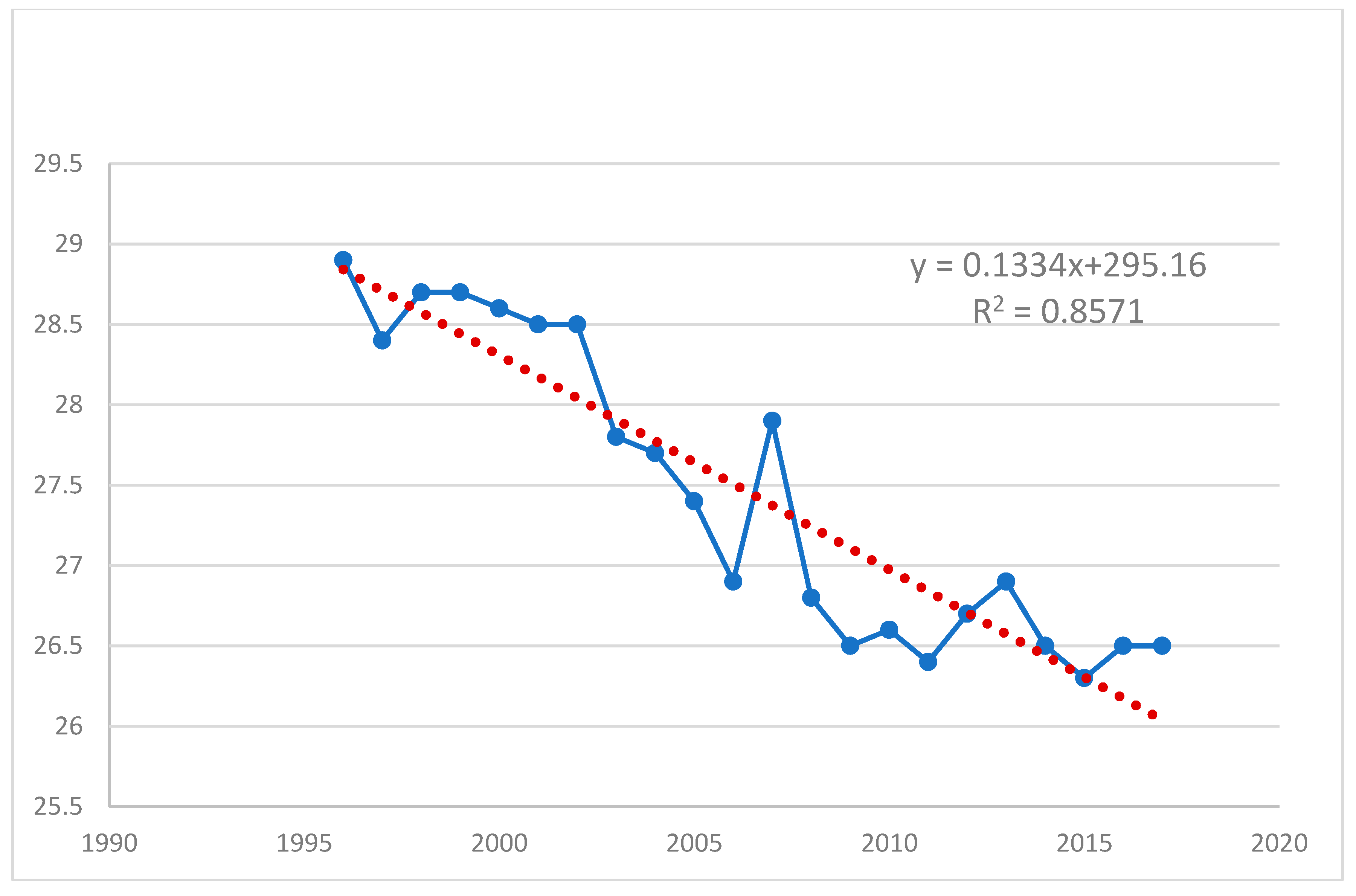
3.1.3. The Trend of Annual Temperature

The trend in annual temperature is shown in Figure 4 below. The trend line shows a general downward trend in movement. A decline in yearly temperature was observed from 1996 to 2005, and then a sharp increase between the years 2006 and 2008. It, however, continues to decline from 2008 to 2017 in an unsteady movement. During the period under study, the minimum annual temperature was recorded to be 26.3 °C in the year 2015, while the maximum yearly temperature was recorded to be 28.9 °C in the year 1996. The mean temperature for the period under study was estimated to be 27.4 °C.
Moreover, the relative variability was calculated to be 24.1%. This implies that variation in temperature for the period under study was not high. The R-squared is estimated to be 0.8571, which is an indication that the trend line fits about 85% of the data values.

3.2. Theoretical Overview and Evaluation of the Climate Change Variables on Yam Production

Looking further, the yields of root and tuber crops, including yam, which is presently on the decline, are predicted to increase in Nigeria towards 2050. As a result of the increase, exports are projected to grow, indicating a projected food surplus for the country (Jalloh et al. 2013). Moreover, impacts of climate change will vary according to location, soil type, crop, and other local factors. Consequently, it is essential to conduct enterprise-specific analysis (Ater and Aye 2012; Sarker et al. 2012). In a review by Knox et al. (2012), it was indicated that for yams, there were too few studies to comment on if there has been any significant impact of climate change on the yield in West Africa. As a result, part of this section attempts to analyze the effects of climate change on yam production in Cross River State.

3.2.1. Stationarity and Non-Stationarity of Time Series

Time series data is made up of observations, which are considered as an understanding of random variables that can be defined by some stochastic processes (Moreira Campos da Cunha Amarante et al. 2018). However, the notion of stationarity is associated with the properties of these stochastic processes. Following Zhang et al. (2019), this study will adopt the concept of weak stationarity. This concept implies that the data series is assumed to be stationary if the properties, such as means, variances, covariances, and autocorrelation of the series, are independent of time (i.e., constant over time), rather than the whole distribution. On the other hand, non-stationarity in a time series arises when the properties, such as the means, or variances, or both, are not constant over time. The most important source of the non-stationarity in time series originates from sources of the unit root (Zhang et al. 2019).

3.2.2. Unit Root (Stationarity) Test

Applying the Johansen’s co-integration technique involves some preliminary testing of the time series to ensure the time series variables are integrated in order one, that is to say, testing for the presence of unit root. Given that time series data are susceptible to spurious regression outcomes, it is crucial to carry out a unit root test before estimating the econometric model (Verter and Bečvářová 2015). In other words, the time series analysis starts by carrying out a unit root test to determine the stationarity or non-stationarity of the variables and to ascertain the suitability of the model specification. Accordingly, the Augmented Dickey–Fuller (ADF) tests were employed to check if each of the variables possesses unit root (that is, to check the stationarity of the data series).
The ADF equation is provided as follows;
ΔYt = δYt−1 + ϵt
where Δ = the first difference operator, δ = (φ − 1) and ϵt denotes a serially uncorrected white noise error term with an average of zero and a constant variance.
The ADF test reduces autocorrelation in the error term because it includes the first difference in lags such that the error term is disseminated as white noise (Eregha et al. 2014). The result of the ADF-test is presented in Table 1. It reveals that all the variables are integrated of order one [I(1)] at level, indicating non-stationarity (presence of unit root) of the time series data. In this circumstance, where the time-series variables under consideration are non-stationary, it, therefore, implies that the result that will be produced by the regression using these variables will be a spurious regression result, except their linear combination provides a stationary residual (Tesso et al. 2012; Zhang et al. 2019).
Moreover, since most of the variables follow order one [I(1)] process (that is, are integrated at the same order), the next stage is to test if there exists a long-run relationship (co-integration) among the variables. Nevertheless, the variables of integrated order one [I(1)] need to undergo first difference before an estimation can be carried out (Sarker et al. 2012; Moreira Campos da Cunha Amarante et al. 2018). However, the study variables became stationary after the first difference exception of the output of yam, which is confirmed by the ADF-test statistics in Table 1. Since the weather series are integrated in the same order, the co-integration technique was employed to ascertain if a stationary long-run relationship exists between the time series. Consequently, the stationarity of the linear combination of the variables in integration order one [I(1)] was tested, and the outcome is presented in the next sub-section using Johansen’s multivariate approach.

3.2.3. Co-Integration Test (Long Term Co-Integrating Relationship)

In a situation of non-stationary time-series, co-integration offers suitable statistical procedures to examine the presence of an economically significant long-term relationship between climate variables (Tesso et al. 2012). Thus, the weather series for stationarity in levels and first difference is tested. In time series econometrics, climate variable that is integrated of order one is represented by Ct~I (1) and climate variable that is integrated in order zero is denoted by ΔCt~I (0). In a case where time series are discovered to be non-stationary at levels, but stationary in first difference, co-integration procedures will probably be implemented (Natanelov et al. 2013). After completion of the unit root test on the time series, and with the assumption that the time series are integrated in the same order, a multivariate Johansen test was conducted on all the variables to investigate co-integration.

3.2.4. Johansen Co-Integration Test Result

The results of the trace statistics from the Johansen co-integration test are shown in Table 2, which suggests a strong rejection of the null hypothesis. The results imply that the hypothesis of no co-integration among the variables can be rejected for the model used. The results further revealed that two co-integrating vectors exist among the study variables in the model. Hence, the rejection of the hypothesis of no co-integrating relationship among the variables under investigation. The result, however, infers that there exists a co-integrating long-run relationship among the time series at 0.05% level of significance. Nevertheless, the trace test indicated that the hypothesis of one co-integrating equation could not be rejected.
As soon as co-integration between time series is recognized, it is crucial to investigate the causality of each co-integrating pair. The causality from the estimated Johansen Vector Error Correction Model (VECM) is evaluated via a likelihood ratio (LR) test by using a restricted disequilibrium error term (Natanelov et al. 2013; Zhang et al. 2019).
Given the presence of long-term relationships recognized among the study variables, the analysis, therefore, undertook an error correction model (ECM) estimation approach. Consequently, the outcome of the ECM is made known in the following sub-section.
In view of the presence of long-term relationships recognized among the study variables, the analysis, therefore, undertook an error correction model (ECM) estimation approach. Consequently, the outcome of the ECM is made known in the following sub-section.
Alternatively, the long run co-integrating relationship was tested using the Engle and Granger technique. The results are shown in Table 3 below. It reveals that the R-squared value of 0.981 (98%) is exceptionally high. Still, the Durbin–Watson statistics are low (1.188), implying that using variables with an ordinary level regression (OLS) will lead to spuriousness.
Furthermore, in examining the residual, which is the Error Correction Model (ECM), the ADF was used to perform unit root on ECM. The result of the test is shown in Table 4 below. The outcome revealed that since the ADF test statistics of −3.37 is significant at 1% level of significance, the null hypothesis of the presence of unit root in ECM was rejected. It, therefore, means that a linear combination of the three non-stationary series is stationary. In other words, the variables are co-integrated. Thus, the study proceeds to the error correction model.

3.2.5. The Outcome from the Error Correction Model

By employing the lag length of three as determined by the information criteria, Table 5 below presents the error correction model result (parsimonious model).
The error correction model results presented in Table 5 specifiy that the model is devoid of any critical econometric hitches. This is so because the Durbin–Watson value of 1.186 indicated the unit root test statistically addressed the existence of positive autocorrelation. Therefore, the Durbin–Watson statistics show the nonappearance of serial correction. The F-statistics value of 2.718, however, conceded the significant test. Simply put, the value of F-statistics suggests that there exists a considerable congruence between each of the climate change variables in the model as the dependent variable and the independent variables are placed together. This implies that the model was statistically fitted at 1% level of probability, which confirms the general explanatory power of the model.
Furthermore, the value of the coefficient of determination of the model clearly showed the goodness of fit. The explanatory variables explained 40% of the variation in output of yam, which was used as the dependent variable in the model. In other words, the R-squared value of 0.404 implied that 40% of the total variation in yam production (dependent variable) was explained by the climate variables (independent variables) included in the model. Thus, the results of the error correction model analysis are reliable and can be used to draw inferences.
Specifically, it can be deduced from the ECM result in line with the theory that climate variables, such as temperature, played a significant role in yam production in the study area. Rainfall was seen to have a positive coefficient but was not statistically significant. The temperature, on the other hand, had a negative impact on yam production in the study area. This implies that a rise in the amount of temperature could result in a decline in yam output in Cross River State. The coefficient (−2.8747) was statistically significant at a 5% probability level, meaning that a 1% increase in temperature will lead to a 28% decrease in yam production. This is true because an increase in temperature encourages the proliferation of pests and diseases, which could be a threat to yam production and yield at the growth and developmental stages. This finding corresponds with the a priori expectation since the temperature has shown a downward trend. In contrast, yam output showed an upward trend during the period under study, implying that as temperature decreases, the quantity of yam produced increases. Hence, the lower the temperature, the higher the quantity of yam produced and vice versa.
However, the Error Correction Model (ECM-1), which signifies the long-run adjustment of the model after disequilibrium, was seen to be statistically significant. The coefficient (−0.477128) of this term specified that, annually, about 48% of the deviation from the equilibrium was adjusted back to stability. In other words, the result from the ECM implies that about 48% of the variation of yam production from its long-run value is corrected. This outcome demonstrates the presence of a strong co-integration, which, in turn, indicates that there is a long-run equilibrium relationship between the study variables.
From previous studies, the assessment of the impact of climate change on China’s rice production was done using the Cobb–Douglas function by Wang et al. (2018). They utilized the daily weather information over the whole growing season for the period 1979–2011. They reported that the minimum temperatures (Tmin), maximum temperatures (Tmax), temperature difference (TD), and precipitation (RP) are the four significant climatic factors that affect rice production in China. They added that except for maximum temperatures, all the factors have positive effects. Similarly, another study was carried out by Samuel et al. (2017) in southwest Nigeria on the impacts of climate variability on agricultural productivity of smallholder farmers. The study discovered that crop yield had reduced tremendously as a result of erratic rainfall, an increase in the number of hours of sunshine, a rise in temperature and pest outbreak.
This finding implies that as the temperature continues to increase over time, it may lead to a decrease in yam production in Cross River State.

3.2.6. Post Regression Test

A post-estimation of the model was carried out, and the result is presented in Table 6 below. The post-regression analysis shows that the model employed is well specified. In the course of estimation, the Durbin–Watson statistic was used to detect the presence of autocorrelation in the model. Any Durbin–Watson statistic outside the range of 1.5–2.5 indicates the presence of autocorrelation (Agwu et al. 2012). Therefore, the Durbin–Watson statistics were estimated to be 1.762265, meaning that there is no autocorrelation detected in the sample. Moreover, the sum squared residual, also known as the residual sum of square, is small (0.045143). This, however, has fulfilled the least square principle that states that the coefficient of sum squared residual is selected such that this value is as small as possible (Moreira Campos da Cunha Amarante et al. 2018).

4. Summary and Conclusions

The findings produced by the research objective one was in two aspects. The first aspect revealed the trend analysis for yam production, annual precipitation, and annual temperature for the period under study. Using the linear trend model, the outcome for yam production revealed an R-squared of 88%. It further showed that there was a steady increase in yam quantity produced between the years 2005 and 2016. The yam production forecast predicts that there will be a sustained increase in yam output for the next 20 years in the study area. This constant higher rates in yam quantity produced may be due to the Structural Adjustment Programme (SAP) in Nigeria, which was introduced into the system around 1986, and some other agricultural policies put in place by the Nigerian government to support agriculture. Concerning the trend in annual precipitation, the outcome of the trend analysis shows the presence of rainfall variability and irregularity in the study area from the unstable movement in trend direction. The R-squared was estimated to be 28%. The annual rainfall was predicted to be on the increase in the next 20 years. As for the trend in annual temperature, the trend analysis estimated the R-squared to be 85%. The trend line showed an overall downward trend in movement, indicating a decline in yearly temperature for the period under study. The annual temperature was forecasted to decrease over the next 20 years continually. In conclusion, the study revealed that for the period under review, an increase in precipitation increased the quantity of yam produced. In contrast, a decrease in temperature increased yam output.
Furthermore, the second aspect of this objective was concerned with the evidence of climate change variables on yam production in Cross River State using the co-integration model. Time series analysis starts by carrying out a unit root test to determine the stationarity or non-stationarity of the variables. The result of the ADF-test carried out showed that all the variables were integrated of order one [I(1)] at level, signifying the presence of unit root in the time series data. For this reason, a test for the presence of a long-run relationship (co-integration) among the variables was done. The outcome of the analysis suggested that there is the presence of co-integrating long-run relationship among the time series at 0.05% level of significance. It revealed a very high R-squared value of 98% and a low Durbin−Watson statistic (1.188), implying that using the variables with an ordinary level regression (OLS) will lead to spuriousness. Therefore, the Error Correction Model (ECM) was employed. The ECM result is in harmony with the literature that climate variables, such as temperature, played a significant role in agricultural production. Rainfall was seen to have a positive coefficient but was not statistically significant. Temperature, on the other hand, was statistically significant and had a negative impact on yam production in the study area.

5. Recommendations

Based on the findings, the research offers the following recommendation:
  • Given the observed adverse effect of temperature on yam production, policymakers need to create an enabling environment for independent researchers as well as institutes to develop pest- and disease-tolerant yam varieties.
  • The agricultural policy to support farmers in Nigeria to concentrate more on the bottom-top participatory approach so that the existing and the developing adaptation practices and technologies could be focused at the farm level since the impact of climate change is crop and location-specific.
  • The government should take appropriate steps to provide an effective weather forecast system that can facilitate the extension of weather information to local farmers to help them know when to expect temperature increase and thus take necessary adaptation action.

6. Limitations of the Study

The study focused on the trends of yam production, precipitation, and rainfall, and also the impact of these climate variables on yam output. No measure was used to take into account labor productivity, capital availability, and production technology, which are factors that may have a role in explaining yam production. Further research should be considered in this direction. Moreover, there was a challenge in collecting time-series data on yam output over a more extended period in Cross River State as there were no documented data before 1996. Therefore, the study used the data available in the state’s database.

Author Contributions

Conceptualization, C.W.A.; data curation, C.W.A.; formal analysis, C.W.A.; funding acquisition, C.W.A.; investigation, C.W.A.; methodology, C.W.A.; resources, C.W.A.; software, C.W.A.; supervision, R.N.B. and A.J.B.; validation, C.W.A., R.N.B., and A.J.B.; visualization, C.W.A., R.N.B., and A.J.B.; writing—original draft, C.W.A.; writing—review & editing, C.W.A., R.N.B., and A.J.B. All authors have read and agreed to the published version of the manuscript.

Funding

The funding for this research was provided by the Niger Delta Development Commission, Nigeria and the Funds for Women Graduate, UK. The Article Processing Charge (APC) for this paper was waived.

Acknowledgments

This paper is part of the Ph.D. research at the Royal Agricultural University, UK. Many thanks to the Niger Delta Development Commission (NDDC), Nigeria and Funds for Women Graduate (FfWG) UK, for providing grants to support this research. Special thanks to the University of Calabar, Nigeria, for granting the corresponding author study leave. We express our gratitude to the Editorial Team of the Journal of Sustainable Development for waiving the APC of this publication.

Conflicts of Interest

The authors declare no conflict of interest.

References

  1. Agwu, Namak, Ifeanyi Nwachukwu, and Cynthia Anyanwu. 2012. Climate variability: Relative effect on Nigeria’s cassava productive capacity. Report Opinion 4: 11–14. Available online: http://www.sciencepub.net/report (accessed on 3 September 2018).
  2. Akinbobola, Temidayo, Tayo Adedokun, and Philip Nwosa. 2015. The impact of climate change on composition of agricultural output in Nigeria. American Journal of Environmental Protection 3: 44–47. [Google Scholar]
  3. Angba, Augustine Oko, Hilda Eta, and Cynthia W. Angba. 2018. Knowledge sharing and learning mechanisms for climate change adaptation among key stakeholders of yam and cassava production in cross river state, Nigeria. Journal of Teaching and Education 8: 177–86. [Google Scholar]
  4. Ater, Peter, and Goodness Aye. 2012. Economic impact of climate change on Nigerian maize sector: A Ricardian analysis. WIT Transactions on Ecology and the Environment 162: 231–39. [Google Scholar] [CrossRef] [Green Version]
  5. Ayinde, OOpeyemi, Mammo Muchie, and Gabriel Olatunji. 2011. Effect of climate change on agricultural productivity in Nigeria: A co−integration model approach. Journal of Human Ecology 35: 189–94. [Google Scholar] [CrossRef]
  6. Cerciello, Massimiliano, Massimiliano Agovino, and Antonio Garofalo. 2019. Estimating urban food waste at the local level: Are good practices in food consumption persistent? Economia Politica 36: 863–86. [Google Scholar] [CrossRef]
  7. Dinar, Ariel, Rashid Hassan, Robert Mendelsohn, and James Benhin. 2008. Climate Change and Agriculture in Africa: Impact Assessment and Adaption Strategies. London: Earthscan, pp. 1–105. [Google Scholar]
  8. Egbe, Cyprian, Margaret Yaro, Asuquo Okon, and Francis Bisong. 2014. Rural Peoples’ Perception to Climate Variability/Change in Cross River State-Nigeria. Journal of Sustainable Development 7: 25–37. [Google Scholar] [CrossRef] [Green Version]
  9. Elijah Samuel, Osuafor Ogonna, and Anarah Samuel. 2018. Effects of Climate Change on Yam Production in Cross River State, Nigeria. International Journal of Agriculture and Forestry 8: 104–11. [Google Scholar]
  10. Enete, Ifeanyi. 2014. Impacts of climate change on agricultural production in Enugu state, Nigeria. Journal of Earth Science & Climatic Change 5: 234. [Google Scholar]
  11. Eregha, Perekunah, Joseph Babatolu, and Rufus Akinnubi. 2014. Climate change and crop production in Nigeria: An error correction modelling approach. International Journal of Energy Economics and Policy 4: 297–311. [Google Scholar]
  12. Geospatial Analysis Mapping and Environmental Research Solutions. 2018. Available online: https://www.gamers.com.ng/map-of-cross-river-state-nigeria/ (accessed on 1 April 2020).
  13. Jalloh, Abdulahi, Gerald Nelson, Timothy Thomas, Robert Zougmore, and Harold Roy-Macauley. 2013. West African Agriculture and Climate Change: A Comprehensive Analysis. Washington: International Food Policy Research Institute, pp. 259–90. [Google Scholar]
  14. Knox, Jerry, Tim Hess, Andre Daccache, and Tim Wheeler. 2012. Climate change impacts on crop productivity in Africa and South Asia. Environmental Research Letters 7: 8. Available online: http://iopscience.iop.org/article/10.1088/1748−9326/7/3/034032/pdf (accessed on 12 March 2017). [CrossRef]
  15. Mbanasor, Jude, Ifeanyi Nwachukwu, Nnanna Agwu, and Ndubuisi Onwusiribe. 2015. Impact of climate change on the productivity of cassava in Nigeria. Journal of Agriculture and Environmental Sciences 4: 138–47. [Google Scholar]
  16. Moreira Campos da Cunha Amarante, Janaina, Tatiana Bach, Wesley Vieira da Silva, Daniela Matiollo, Alceu Souza, and Claudimar Pereira da Veiga. 2018. Econometric analysis of co-integration and causality between market prices toward futures contracts: Evidence from the live cattle market in Brazil. Cogent Business & Management 5: 1457861. [Google Scholar] [CrossRef]
  17. Natanelov, Valeri, Andrew McKenzie, and Guido Van Huylenbroeck. 2013. Crude oil-corn-ethanol-nexus: A contextual approach. Energy Policy 63: 504–13. [Google Scholar] [CrossRef]
  18. National Population Commission (NPC). 2011. Census enumeration survey N. P. C. Abuja, Nigeria. Federal Government Statistical Bulletin 2: 6–8. [Google Scholar]
  19. Nwaobiala, Chioma, and Do Nottidge. 2015. Effect of climate variability on output of cassava in Abia State, Nigeria. Nigeria Agricultural Journal 46: 81–86. [Google Scholar]
  20. Samuel, Ogalloh, Wandiga Shem, Olago Daniel, and Oriaso Silas. 2017. Impacts of climate variability and climate change on agricultural productivity of smallholder farmers in Southwest Nigeria. International Journal of Scientific & Engineering Research 8: 128–32. [Google Scholar]
  21. Sarker, Md. Abdur Rashid, Khorshed Alam, and Jeff Gow. 2012. Exploring the relationship between climate change and rice yield in Bangladesh: An analysis of time series data. Agricultural Systems 112: 11–16. [Google Scholar] [CrossRef]
  22. Tesso, Gutu, Bezabih Emana, and Mengistu Ketema. 2012. A time-series analysis of climate variability and its impacts on food production in North Shewa zone in Ethiopia. African Crop Science Journal 20: 261–74. [Google Scholar]
  23. Thomas-Hope, Elizabeth. 2017. Climate Change and Food Security: Africa and the Caribbean. Amsterdam: Routledge, pp. 1–112. [Google Scholar]
  24. Verter, Nahanga, and Věra Bečvářová. 2015. An Analysis of Yam Production in Nigeria. Acta Universitatis Agriculturae et Silviculturae Mendelianae Brunensis 63: 659–65. [Google Scholar] [CrossRef] [Green Version]
  25. Wang, Dan, Yu Hao, and Jianpei Wang. 2018. Impact of climate change on China’s rice production—An empirical estimation based on panel data (1979–2011) from China’s main rice-producing areas. The Singapore Economic Review 63: 535–53. [Google Scholar] [CrossRef]
  26. Zhang, Rongmao, Peter Robinson, and Qiwei Yao. 2019. Identifying co−integration by eigenanalysis. Journal of the American Statistical Association 114: 916–27. [Google Scholar] [CrossRef]
Figure 1. Map of Cross River State showing the 18 Local Government Areas. Source: Geospatial Analysis Mapping and Environmental Research Solutions (2018).
Socsci 09 00042 g001
Figure 2. Trend analysis plot for yam output in Cross River State. Source: Author’s computation from data obtained from NPAFS and FMW&WR.
Socsci 09 00042 g002
Figure 3. Trend analysis plot for annual rainfall (MM) in Cross River State. Source: Author’s computation from data obtained from CBN.
Socsci 09 00042 g003
Figure 4. Trend analysis plot for annual temperature (°C) in Cross River State. Source: Author’s computation from data obtained from CBN.
Socsci 09 00042 g004
Table 1. Results of unit root test from the Augmented Dickey–Fuller Test.
Variables@ Level1st DifferenceDecision
ADF Statisticsp-ValueOrder of IntegrationADF Statisticsp-ValueOrder of Integration
Yam output−2.2620920.4335I(1)−2.5769550.2927I(1)Non-stationary
Rainfall−3.5263590.0623I(1)−4.7251980.0069 ***I(0)Stationary
Temperature−3.0005570.1550I(1)−4.5831920.0091 ***I(0)Stationary
Source: Author’s computations from data obtained from CBN, NPAFS and FMW≀ Note that *** indicates rejection of the null hypothesis (presence of a unit root) at 5% level of significance.
Table 2. Unrestricted Cointegration Rank Test (Trace).
Hypothesized No. of CE(s)EigenvalueTrace Statistic0.05 Critical ValueProb.
None *0.74956.9847.8560.005
At most 1 *0.56230.7229.7970.039
At most 20.44415.0415.4950.068
At most 3 *0.1843.8813.8410.048
Source: Author’s estimation. Trace test indicates two cointegrating equations at the 0.05 level. * denotes rejection of the hypothesis at the 0.05% level. Note that None = (r ≤ 0), At most 1 = (r ≤ 1), At most 2 = (r ≤ 2), At most 3 = (r ≤ 3).
Table 3. Long run relationship (OLS regression).
VariableCoefficientStd. Errort-StatisticsProb.
C14.4283.5534.0600.000
LOG(AVRAINFALL)0.1500.1491.0100.326
LOG(AVTEMP)−3.4200.991−3.4520.003
R-Squared0.981Mean dependent variable7.730
Adjusted R-Squared0.979S.D. dependent variable0.550
SE of Regression0.080Akaike info criterion−2.047
Sum Squared Residual0.116Schwarz criterion−1.848
Log-Likelihood26.512Hannan–Quinn criterion−1.999
F-Statistic323.743Durbin–Watson statistic1.188
Prob(F-Statistic)0.000
Source: Author’s estimation.
Table 4. ADF unit root test on ECM.
VariableCoefficientStd. Errort-StatisticProb.
ECM(−1)−0.7790.231−3.3720.003
D(ECM(−1))0.3530.2041.7290.100
R-Squared0.386Mean dependent variable0.003
Adjusted R-Squared0.352S.D. dependent variable0.079
SE of Regression0.063Akaike info criterion−2.572
Sum Squared Residual0.073Schwarz criterion−2.472
Log-Likelihood27.72Hannan–Quinn criterion−2.552
Source: Author’s estimation.
Table 5. Results from the Error Correction Model.
VariableCoefficientStd. Errort-StatisticProb.
C0.0120.0230.5520.588
DLOG(AVRAINFALL)0.1190.1041.1400.271
DLOG(AVTEMP)−2.8751.159−2.4790.025 **
ECM(−1)−0.4770.269−1.7714660.0955 *
R-Squared0.405Mean dependent variable0.064
Adjusted R-Squared0.256S.D. dependent variable0.085
SE of Regression0.073Akaike info criterion−2.181
Sum Squared Residual0.086Schwarz criterion−1.933
Log-Likelihood27.909Hannan–Quinn criterion−2.128
F-Statistic2.718Durbin–Watson statistics1.287
Prob(F-Statistic)0.067
Source: Author’s computation (Note that ** and * indicate that the test statistics are significant at 5% and 10% respectively).
Table 6. Post regression test result.
VariableCoefficientStd. Errort-StatisticProb.
C0.0187010.0194140.9632380.3518
DLOG(AVRAINFALL)−0.0348800.081811−0.4263420.6763
DLOG(AVTEMP)0.1188220.9000550.1320160.8968
ECM(−1)−1.2745330.451685−2.8217320.0136
RESID(−1)1.6738030.4827093.4675210.0038
RESID(−2)0.3871200.3125561.2385620.2359
R-squared0.476140Mean dependent variable7.23 × 10−18
Adjusted R-squared0.251629SD dependent varvariable0.065641
SE of Regression0.056785Akaike info criterion−2.637900
Sum Squared Residual0.045143Schwarz criterion−2.289726
Log-Likelihood34.69795Hannan–Quinn criterion−2.562337
F-Statistic2.120784Durbin–Watson statatistic1.762265
Prob(F-Statistic)0.115641
Source: Author’s computation.

