1. Introduction
In recent years, the term circular economy has gained much attention. It refers to a system of production and consumption providing minimal losses of materials and energy through extensive reuse, recycling, and recovery
Haupt et al. (
2017). In other words, it is an economic system for which is essential to recycle materials from waste in order “to close the cycle”.
Waste disposal should be gradually eliminated, and where this is not possible, it should be monitored in order to be safe for human health and the environment. Consequently, solid waste management increasingly represents a challenge since municipalities must provide an efficient system to their population. However, they often have to struggle with complexity and with lack of both organization and financial resources
Burntley (
2007).
Among other things, sustainable waste management is able to reduce the incidence of health problems, the emission of greenhouse gases, and the deterioration of landscape, water, and air caused by landfilling
Cucchiella et al. (
2017). However, it not only represents a contribution to environmental protection, but it also pays off economically
Nelles et al. (
2016): waste management practices, indeed, can be cost-saving and generate revenue opportunities
Romero-Hernández and Romero (
2018).
In fact, waste can be a useful source of raw materials and energy, too. Metals, glass, and textiles have long been collected and put to new use; for example, the extraction of nickel and cobalt from raw materials, as well as from waste, is strategically important for industry and society
Komnitsas et al. (
2019). Waste can be turned into energy too, enabling the value of products, materials, and resources to be maintained on the market for as long as possible, minimizing waste and resource use in the wake of the objectives of circular economy
Malinauskaite et al. (
2017).
For all these reasons, and since the circular economy is an important issue for the future and the competitiveness of businesses
Garcia-Muiña et al. (
2018), solid waste management might represent an opportunity for the municipal authorities of developing countries, especially those characterized by a low-income
Minghua et al. (
2009).
In conclusion, in a circular economy wastes are considered a resource, especially from an economic point of view, consequently attracting an increasing number of industrial actors, policy-makers, and researchers
Cucchiella et al. (
2017). Thus, in the last years, a large number of studies have tried to detect factors influencing waste management systems in developing countries.
From our analysis, it may be concluded that a study of this kind offers a potential pathway for academics to work with policy-makers in moving toward the realization of waste management policies tailored to the local context.
2. Materials and Methods
Real data often consists of mixed variables, that is, both continuous and categorical ones; an example is provided by the dataset analyzed in this paper, produced by
Abarca-Guerrero (
2014), the variables of which are described in
Table 1. Traditionally, cluster analysis has only focused on datasets composed of a single type of variable (all quantitative or all qualitative). For this reason, researchers dealing with mixed data usually convert them into a single data type, transform the categorical variables into binary ones and consequently apply methods for numeric variables, or transform continuous variables into categorical ones
Dougherty et al. (
1995);
Ichino and Yaguchi (
1994).
Indeed, clustering methods specific to mixed data are less encountered in the literature.
Some traditional methods are:
data pre-processing, that is, all variables are converted to the same scale, either numerical to categorical or vice-versa;
distance measures specifically developed for mixed datasets.
With regards to data pre-processing, these algorithms are essentially created for purely categorical attributes, although they have also been applied to mixed data after a transformation of numerical attributes to categorical ones (discretization). In general, these kinds of algorithms can be applied to mixed data through a discretization process that may, nevertheless, produce a loss of important information
Caruso et al. (
2018).
One example is represented by the dummy coding of all categorical variables. But this increases the dataset’s dimensionality, representing a problem when the number of categorical variables simultaneously increases with the size of the data. Another disadvantage is that any semantic similarity in the original dataset is lost in the transformed one. Finally, coding strategies imply a difficult choice of weights representing categorical attributes
Foss et al. (
2016).
An alternative to recoding categorical or continuous variables is to use a dissimilarity measure, taking into account the different types of data
Caruso (
2019). A common approach is to use the Gower distance
Gower (
1971).
2.1. Clustering Mixed Data
Let denote a set of n objects and indicate an object constituted by L variables. Since the L variables of the considered dataset are both continuous and categorical, it is possible to write , where Q corresponds to the number of numeric variables and C to the number of categorical ones. is a subset identifying the qualitative variables and is a subset denoting the quantitative ones. The aim of clustering is to assign the n objects contained in X to K separate clusters. When clustering mixed datasets, the main problem is to determine how close or how far apart objects are from each other.
2.2. The Huang Method
Huang (
1998) presented a so-called K-prototypes algorithm, which is based on the K-means method but overcomes its quantitative data limitation, preserving, at the same time, its efficiency. The algorithm groups the objects in clusters against k prototypes. The updates occur in a dynamical manner, so as to minimize the following objective function:
where
is an element of a partition matrix
, and
is a dissimilarity measure for mixed data between the objects
and
.
is the prototype or representative vector for cluster k. U represents a hard partition matrix, where , and if is allocated to cluster k.
The Huang dissimilarity measure for mixed data is defined as
where the first term is the squared Euclidean distance, whereas the second one is defined as
for
and
for
.
is a weight for categorical variables in cluster
k.
The internal term in Equation (
1) can be defined as
. It measures the total dissimilarity of objects in cluster
k from their prototype
. The quantity
could be considered as the total cost of allocating the objects
to cluster
k.
This term may be rewritten as
where
and
represent the dissimilarity of the objects in cluster
k for the quantitative and the qualitative variables, respectively. In order to minimize these two components, let
and
be the prototypes for cluster
k for the numerical and categorical variables, respectively.
is minimized with the usual update of the K-means algorithm for continuous variables. That is, the generic component of
is the arithmetic mean:
where
is the number of objects in cluster
k. Let
be the set enclosing the distinct values of the
l-th categorical variable, and let
be the probability that value
is observed in cluster
k.
It is possible to rewrite
in (
3) as
In Equation (
5),
is minimized by selecting the categorical values of the prototype
, such that
for
for all categorical variables.
On the basis of the Huang algorithm, by minimizing (
1), we implemented a cluster analysis with a number of clusters equal to
. This choice was made based on the Silhouette index
Rousseeuw (
1987); since higher values corresponds to better results, the resultant (optimal) maximum value precisely corresponds to 2.
4. Discussion
On the basis of our analysis of quantitative variables, it appears that the first cluster is characterized by a lower percentage of urban population, lower levels of GDP, and a lower life expectancy. As a consequence of limited urbanization and greater poverty, this group registers lower rates of waste generation and of
emissions. Since the cluster discrimination between the two groups is well defined, the second cluster registers the opposite tendency for all of the above-mentioned variables, namely higher levels of GDP and a stronger percentage of urban population, with a consequently higher life expectancy. The higher urbanization corresponds to higher levels of waste generation and of
emissions. In more detail, in order to better describe the distribution of the quantitative variables analyzed, each of these has been represented through a box plot
Cleveland (
1993).
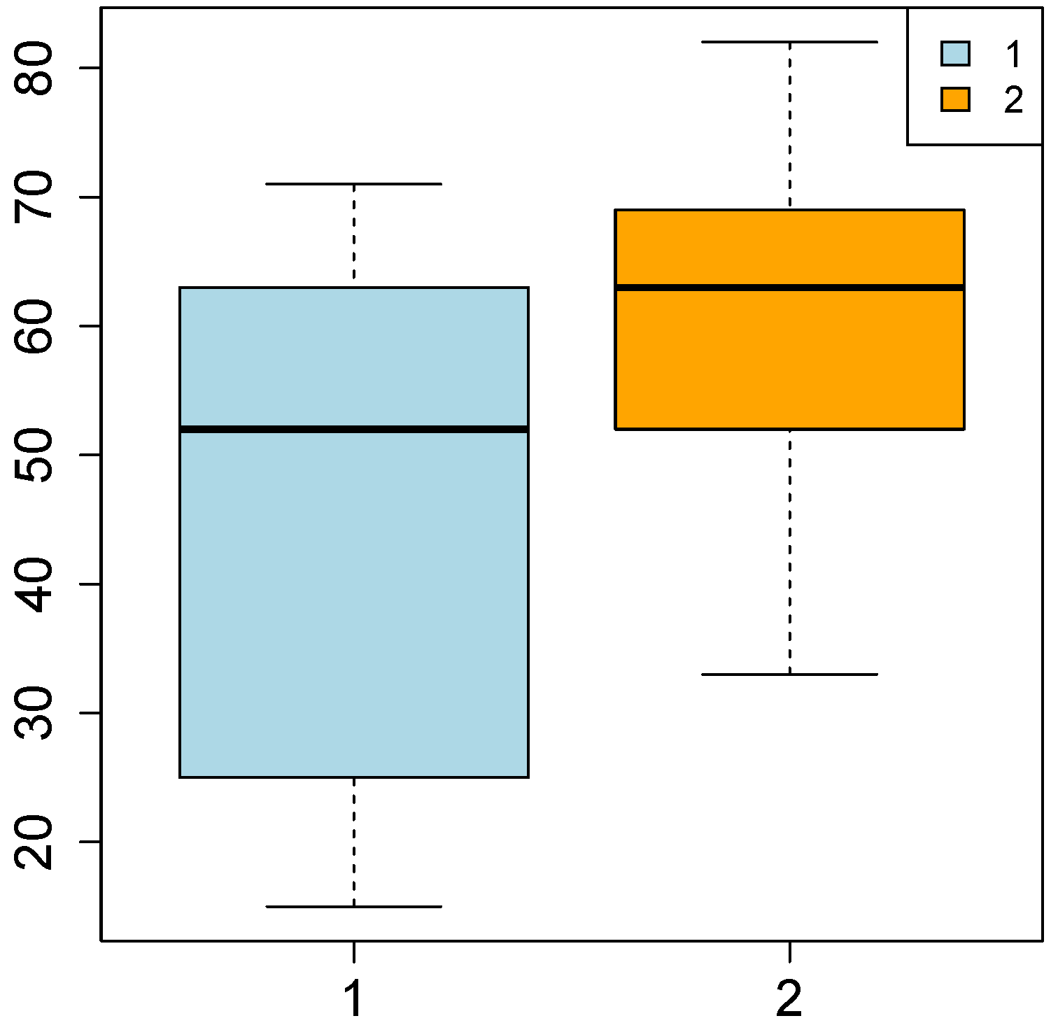
With regards to the percentage of urban population (
Figure 1), the overall median of the distribution equals 57.00, whereas the overall mean is 51.12; the mean of the first cluster is lower than this, whereas the one associated with the second cluster is higher. In the first cluster, the interquartile distance is much higher than in the second one, denoting a greater dispersion of the
most central observations around the median. On the other hand, since the interquartile distance of the second cluster is lower, the
most central observations are highly concentrated around the median. Furthermore, since in the first cluster the distances between each quartile and the median are quite different from one another, the distribution is asymmetric. In the second cluster, instead, the distances are more similar between these, denoting a lower asymmetry of the distribution.
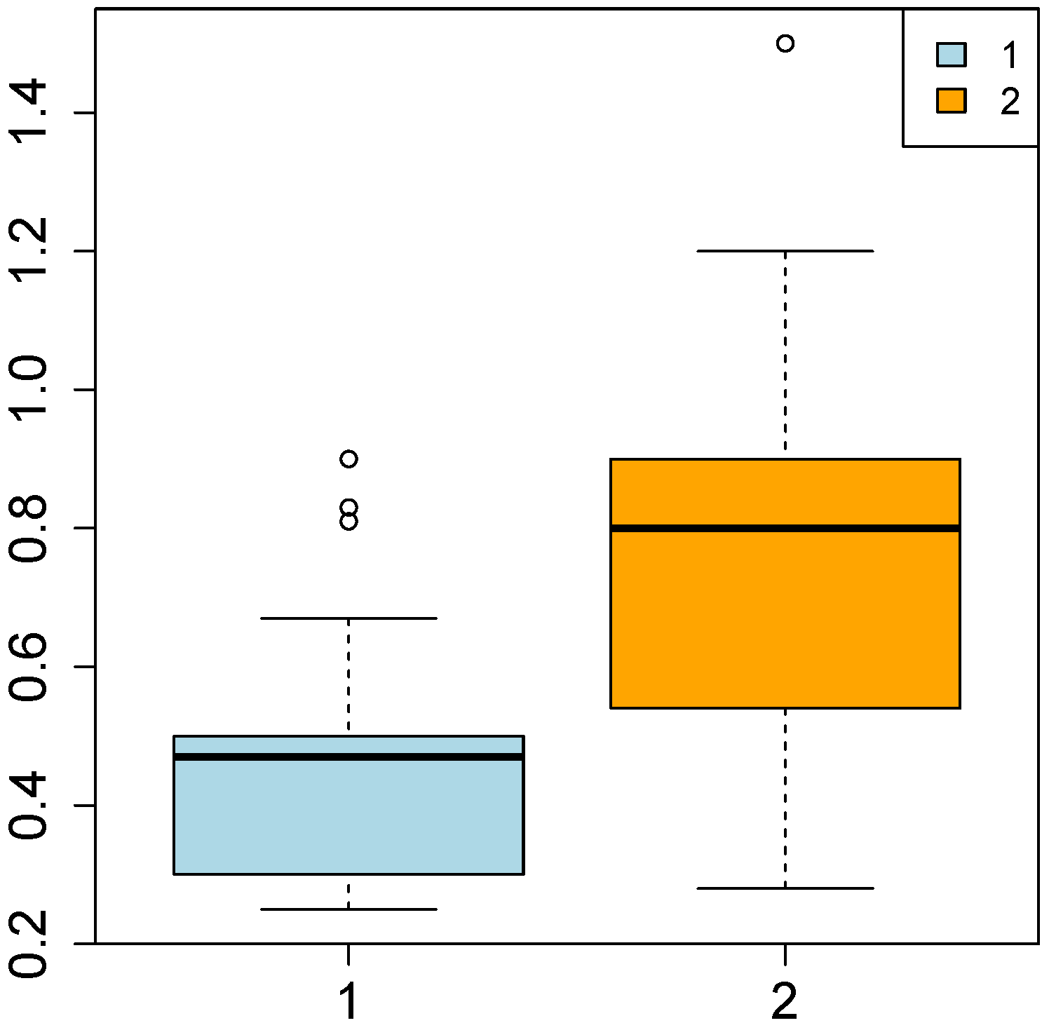
For what concerns the waste generation (
Figure 2), the overall median of the distribution equals 0.50, whereas the overall mean is 0.61; the mean of the first cluster is lower than this, whereas the one associated with the second cluster is higher. In the first cluster, the interquartile distance is lower than in the second one. Thus, in the first group there is a low dispersion of the
most central observations around the median. On the other hand, since the interquartile distance of the second cluster is higher, the
most central observations are less concentrated around the median. Furthermore, in the first cluster the two distances are quite different from one another, denoting a very asymmetric distribution, whereas in the second group these distances are more similar, resulting in a slightly lower asymmetry of the distribution.
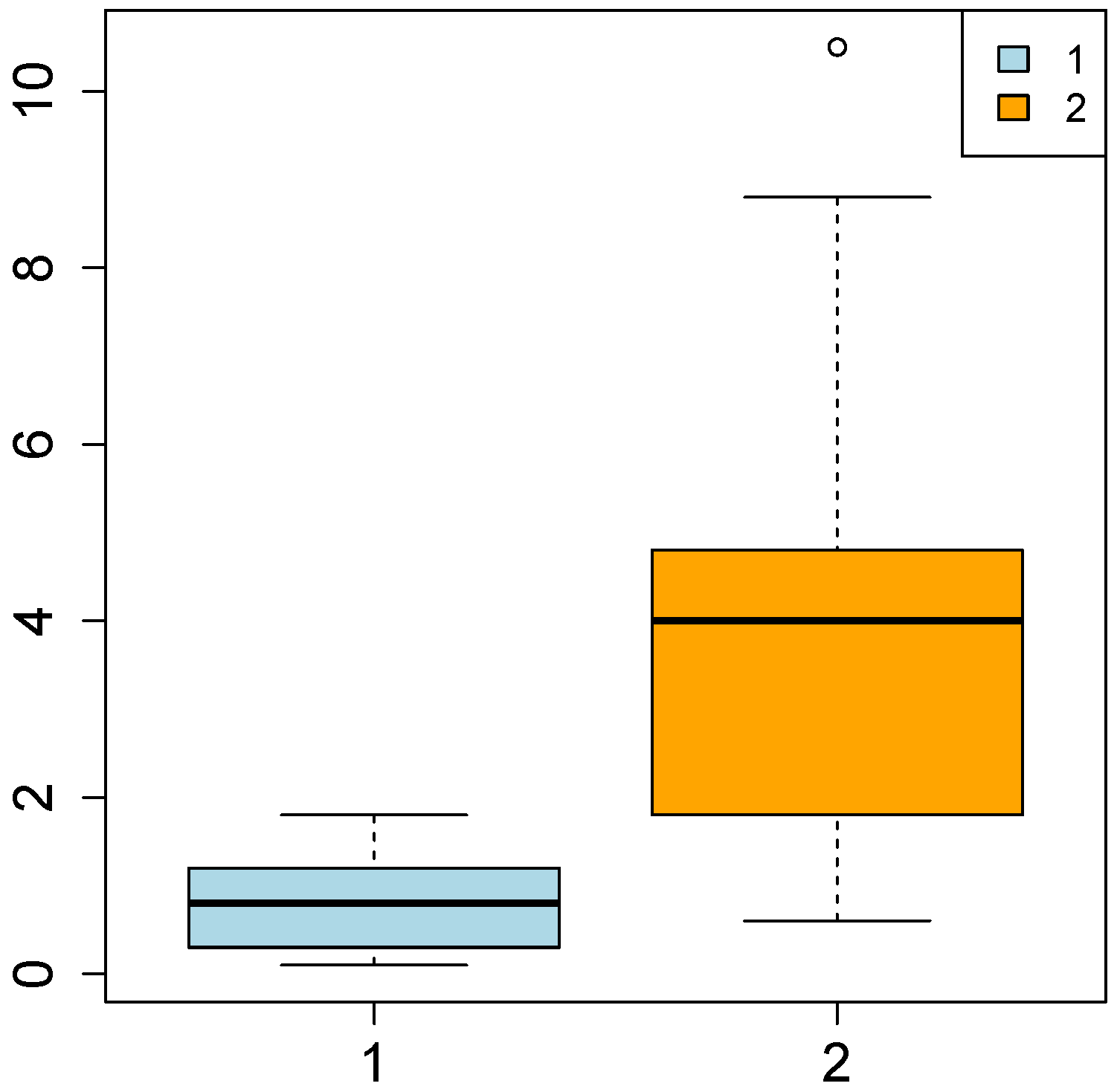
With regards to the
emissions (
Figure 3), the overall median of the distribution equals 1.40, whereas the overall mean is 2.28; the mean of the first cluster is lower than this, whereas the one associated to the second cluster is higher. In the first cluster, the interquartile distance is lower than in the second one. Thus in the first group, the dispersion of the
most central observations around the median is lower. On the other hand, since the interquartile distance of the second cluster is higher, the
most central observations are less concentrated around the median. Furthermore, in the first cluster the two distances are very similar to one another, denoting a symmetric distribution, whereas in the second cluster they are less similar, indicating the asymmetry of the distribution.
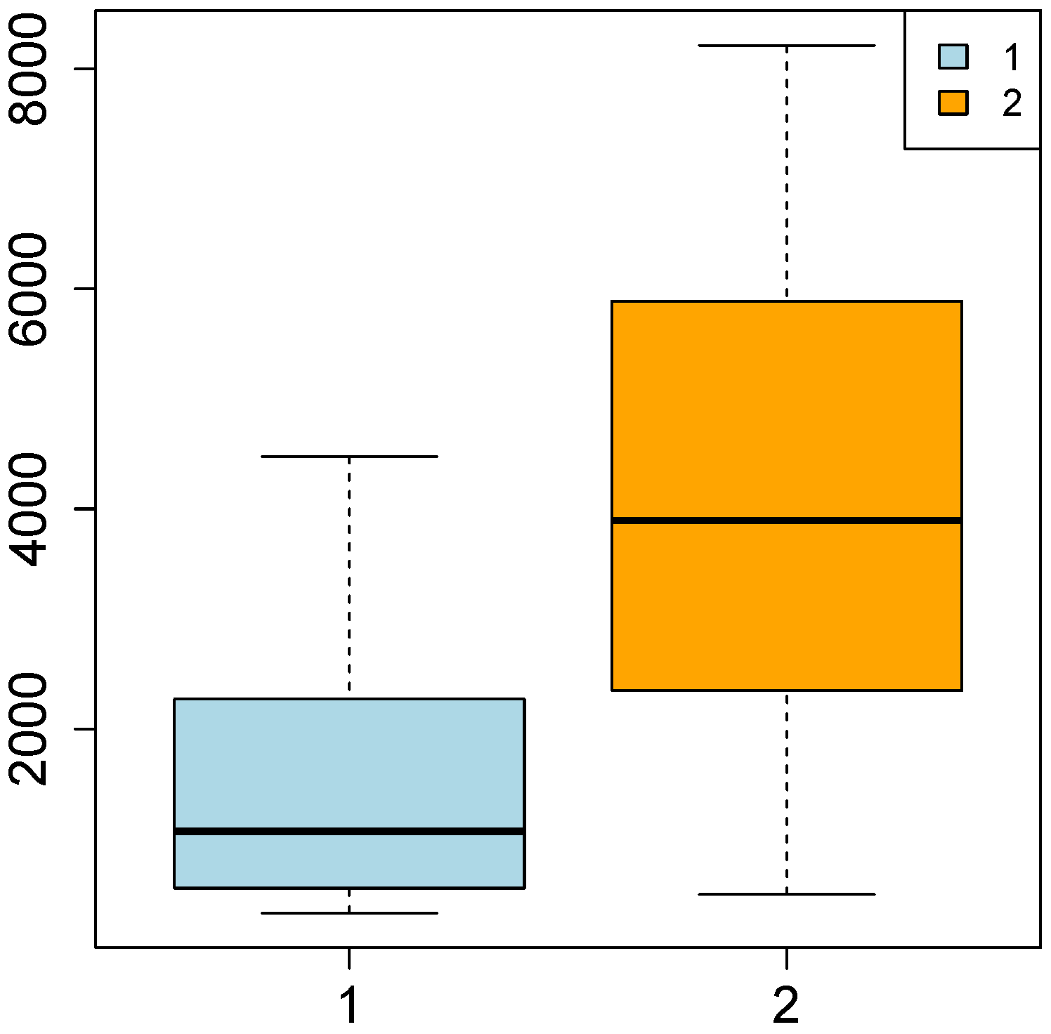
With regards to the GDP (
Figure 4), the overall median of the distribution equals 2349, whereas the mean is 3825; the median of the first cluster is lower than this, whereas the one associated with the second cluster is higher. In the first cluster, the interquartile distance is lower than in the second one. Thus, in the first group the dispersion of the the
most central observations around the median is lower. Since the interquartile distance of the second cluster is higher, instead, the
most central observations are less concentrated around the median. Furthermore, in the first cluster the two interquartile distances are quite different from one another, so the distribution is asymmetric. In the second cluster, instead, they are more similar, denoting the lower asymmetry of the distribution.
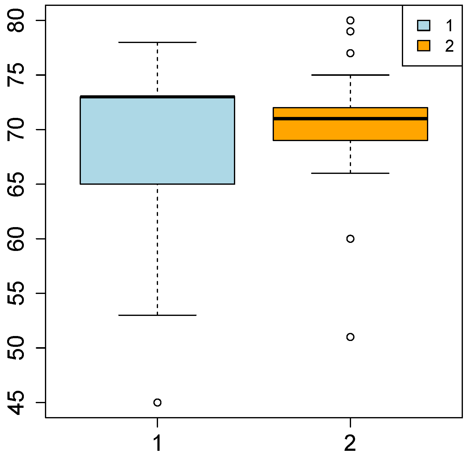
For what concerns life expectancy (
Figure 5), the overall median of the distribution equals 71.00, whereas the overall mean is 68.46, thus the mean of the first cluster is lower than this, whereas the one associated with the second cluster is higher. In the first group, the interquartile distance is higher than in the second one. Thus, in the first group the dispersion of the
most central observations around the median is higher. On the other hand, since the interquartile distance of the second cluster is lower, the
most central observations are highly concentrated around the median. Furthermore, in the first cluster the two distances are quite different from one another, so the distribution is asymmetric, whereas in the second group the distances are more similar, denoting the lower asymmetry of the distribution.
With regards to qualitative variables, instead, the first cluster is characterized by the overwhelming majority of recycling awareness campaigns supported by the municipality, the waste is mainly collected through animal power, and there are some recyclable-material-buying companies and some recycling companies in the surrounding areas of the cities. The countries falling under this category are mostly characterized by monsoonal precipitation and are the following: Ethiopia, Sri Lanka, Thailand, China, Peru, Tanzania, India, Bangladesh, Nepal, Malawi, Zambia, Nicaragua, Kenya, and the Philippines.
The second cluster, instead, is mainly characterized by the absence of recycling awareness campaigns supported by the municipality, the waste is mainly collected through mechanized tools, but it is mostly characterized by the absence of recyclable-material-buying companies and of recycling companies in the surrounding areas of the cities. Furthermore, it is characterized by the prevalence of a fully humid climate. The countries falling into this cluster are Turkey, Suriname, Costa Rica, Ecuador, Pakistan, and Bhutan, whereas Indonesia and South Africa are in the overlapping area of the two clusters.
5. Conclusions
Since nowadays more and more applications are based on datasets composed of mixed data, there is an ever-growing interest in cluster analysis. Due to their characteristics, traditional methods are unable to capture, store, manage, and analyze these datasets. A cluster analysis implemented on such a dataset has huge potential; however, most clustering algorithms are designed to exclusively handle one type of data at a time, being unable to analyze mixed data simultaneously. The use of cluster analysis for mixed data represents an element of innovation, especially in the waste management sector, since until now only the traditional cluster analysis has been applied in this framework.
Certainly, the research in this area is far from being complete. There are quite a few methods in the literature, but further advancements in this field are needed
Caruso (
2019). Furthermore, in the wake of this work, future research will be focused on the development of new cluster analysis techniques for mixed data and on the consequent creation of dedicated software packages, also with the aim of widening the number of potential users of this method
Caruso et al. (
2019).
The basis for future developments will take into consideration the results yielded from the applications described in
Section 3 and from an interesting insight provided by the work of Diday and Govaert
Diday and Govaert (
1977). They propose an adaptive clustering that consists in a dynamic procedure and is useful for calibrating the weights of variables used in the clustering.
Usually, indeed, all of the variables participate in the cluster analysis with the same importance, but since some of them may be more discriminant than others, or better characterize a cluster, there are some ways to correctly consider their different values
Irpino et al. (
2016).
One strategy consists in assigning a weight to each variable in advance, on the basis of a prior knowledge, and then performing a cluster analysis; a future development could consist in computing the weights for each variable in an automatic way
Caruso (
2019). In this context, Diday and Govert
Diday and Govaert (
1977) proposed using an adaptive distance when clustering real data. It is necessary to introduce a weighting step in the optimization process, generating a set of weights; each of these corresponds to a variable and measures its importance in the cluster analysis. While Diday and Govert’s proposal is only focused on quantitative variables, a further advancement could be to extend it to both quantitative and qualitative data.
