Article

Googling Fashion: Forecasting Fashion Consumer Behaviour Using Google Trends

1
Centre for Fashion Business and Innovation Research, Fashion Business School, London College of Fashion, University of the Arts London, 272 High Holborn, London WC1V 7EY, UK
2
Research Institute of Energy Management and Planning, University of Tehran, Tehran 1417466191, Iran
3
Department of Business, Marketing and Law, School of Business, University of South-Eastern Norway, Bredalsveien 14, 3511 Hønefoss, Norway
4
Centre for Fashion Business and Innovation Research, Fashion Business School, London College of Fashion, University of the Arts London, 272 High Holborn, London WC1V 7EY, UK
*
Author to whom correspondence should be addressed.
Soc. Sci. 2019, 8(4), 111; https://doi.org/10.3390/socsci8040111
Submission received: 22 February 2019 / Revised: 25 March 2019 / Accepted: 29 March 2019 / Published: 4 April 2019
(This article belongs to the Special Issue Fashion Merchandising and Consumer Behavior)

Abstract

:
This paper aims to discuss the current state of Google Trends as a useful tool for fashion consumer analytics, show the importance of being able to forecast fashion consumer trends and then presents a univariate forecast evaluation of fashion consumer Google Trends to motivate more academic research in this subject area. Using Burberry—a British luxury fashion house—as an example, we compare several parametric and nonparametric forecasting techniques to determine the best univariate forecasting model for “Burberry” Google Trends. In addition, we also introduce singular spectrum analysis as a useful tool for denoising fashion consumer Google Trends and apply a recently developed hybrid neural network model to generate forecasts. Our initial results indicate that there is no single univariate model (out of ARIMA, exponential smoothing, TBATS, and neural network autoregression) that can provide the best forecast of fashion consumer Google Trends for Burberry across all horizons. In fact, we find neural network autoregression (NNAR) to be the worst contender. We then seek to improve the accuracy of NNAR forecasts for fashion consumer Google Trends via the introduction of singular spectrum analysis for noise reduction in fashion data. The hybrid neural network model (Denoised NNAR) succeeds in outperforming all competing models across all horizons, with a majority of statistically significant outcomes at providing the best forecast for Burberry’s highly seasonal fashion consumer Google Trends. In an era of big data, we show the usefulness of Google Trends, denoising and forecasting consumer behaviour for the fashion industry.

1. Introduction

The emergence of big data and advances in big data analytics led to the creation of Google Trends (Choi and Varian 2012), a tool and source for analysing big data on web searches across the globe. Given that 70% of luxury purchases are estimated to be influenced by online interactions (D’Arpizio and Levato 2017), Google Trends has the potential to play a pivotal role in the developments of big data in fashion. Fashion consumers are actively using Google, looking for ideas, finding the best designs, and buying with a tap (Boone 2016). In 2016 alone, Google was receiving more than 4 million search queries per minute from 2.4 billion internet users and was processing 20 petabytes of information per day (Wedel and Kannan 2016). Data analytics on such online behaviour lets Google predict the next big fashion trend (Bain 2016) with Google’s Online Retail Monitor indicating that in 2018, fashion has seen the highest growth in searches, boosted by overseas shoppers (especially from the EU) seeking access to UK brands online (Jahshan 2018). Such trends are positive for the fashion industry in the UK which is experiencing considerable uncertainty with Brexit looming on the horizon.
Google Trends is a good example of how big data can be exploited and visualised in a user-friendly style. The term big data itself struggles to find a universal definition and it can mean different things to different people (Marr 2015; Hassani and Silva 2015b). Nevertheless, most researchers agree on building upon the three defining dimensions of Big Data (3Vs) as introduced by Laney (2001): volume, variety and velocity. Figure 1 below summarises the 3Vs to give the reader an indication on how big data was initially thought to be expanding. Today, the definition of big data has evolved (much like the size of big data which has only gotten bigger as predicted by Varian 2014) and now includes 5Vs, with additional Vs being veracity (which accounts for the quality of the data) and value (which accounts for analytics on data) (Hassani and Silva 2018).
It is no secret that Google Trends are increasingly influencing business decision-making in a variety of industries (see, for example, Yu et al. 2019; Siliverstovs and Wochner 2018; Zhang et al. 2018) given its ability to act as a leading indicator for forecasting key variables of interest. The fashion industry too can benefit from the exploitation of Google Trends for forecasting fashion variables, from predicting future purchase decisions, to determining the effectiveness of marketing campaigns and forecasting online consumer brand engagement. Moreover, there is a need for more conclusive research which evaluates whether big data in the form of Google Trends can help predict actual sales for fashion brands. Whilst finding the answer to this problem is beyond the scope of our research, there is reason to believe that this could be the case, since evidence suggests that Google searches can predict other types of economic activity such as real estate sales and prices (Wu and Brynjolfsson 2015), exchange rates (Bulut 2018), UK cinema admissions (Hand and Judge 2011), stock market volatility (Hamid and Heiden 2015), inflation expectations (Guzman 2011) and tourist arrivals (Bangwayo-Skeete and Skeete 2015). In addition, there could be several alternate research avenues which are waiting to be explored not only from a fashion design, buying and merchandising perspective, but also from a fashion management perspective (see, for example, Madsen 2016), particularly in evaluating the success of marketing and social media campaigns.
We subscribe to Gordon’s (2017) view that Google Trends can be a metric for online consumer behaviour, as more than 75% of the world’s internet searches are conducted on Google (Net Market Share 2019). Therefore, we believe that the fashion industry should consider relevant Google Trends as ‘fashion consumer Google Trends’ which according to McDowell (2019) can enable brands to identify consumer patterns and profit from them. Here, it is worthwhile to define Google Trends for the reader. In brief, as one of the largest real time datasets currently available (Rogers 2016), recording Google search data from 2004 to present (Choi and Varian 2012), Google Trends allows one to gauge consumer search interest in brands. However, instead of the raw level of queries for a given search term, it is important to note that Google Trends reports the query index, which begins with a query share (Choi and Varian 2012):
Total   query   volume   for   search   term   in   a   given   geographic   location Total   number   of   queries   in   that   region   at   a   point   in   time
In other words, its normalised nature (which enables more accurate comparisons over time) means that Google Trends will always show the search interest on a topic as a proportion of all searches on all topics on Google at that time and location (Rogers 2016). Data quality is another important consideration, and Google Trends seeks to improve the quality of its data by excluding searches made by very few people, duplicate searches and special characters (Google 2019; Choi and Varian 2012). Furthermore, the query share based approach to computing Google Trends has its benefits in a world where big data and data mining have been marred by privacy issues and concerns (Hassani et al. 2014, 2016a). The data aggregation underlying Google Trends ensures the output is anonymised and thus no individual is identified personally (Rogers 2016).
The motivations for this research (and its importance) stems from several existing studies. Firstly, Jun et al. (2018) notes that the purpose of big data utilisation is now shifting from monitoring towards forecasting, and thereby, indicating the importance of predictive analytics and forecasting for the future. Secondly, the increase in ‘research shopping’, whereby consumers are seen accessing information via one channel and purchasing through another channel (Verhoef et al. 2007; Bradlow et al. 2017), adds more importance to the potential of fashion consumer Google Trends to be a useful fashion analytics tool. Thirdly, as LaValle et al. (2011) points out, organisations are interested in what is likely to happen next, and forecasting is a tool which can provide this information. However, the emergence of big data brings about its own challenges for generating accurate forecasts (Hassani and Silva 2015b). Fourthly, Wedel and Kannan (2016) assert that trend forecasting is vital for companies to be able to identify changes in the environment and set up defences to retain market share. Furthermore, the fashion industry currently benefits from big data trend forecasts and analytics through popular and well reputed services by WGSN and Edited. As discussed later, Google Trends has the potential to complement these existing platforms. To this end, Google Trends can indicate consumer sentiment towards a brand, and has the ability to extrapolate this to potential purchasing behaviour that can help brands plan more effectively.
Thus, our interest lies in understanding the benefits of Google Trends for fashion analytics and identifying the possibility of forecasting such online consumer trends into the future so that more productive managerial and marketing decisions can be made. Accordingly, the aim of this paper is to determine whether there exists a single univariate forecasting model which can predict fashion consumer Google Trends across both short and long run horizons. The following objectives are put forward to help achieve this aim. (1) Identify the uses of Google Trends for predicting fashion consumer behaviour and the need for forecasting same, (2) analyse parametric and nonparametric univariate time series models at forecasting fashion consumer Google Trends and (3) evaluate the importance of signal extraction and denoising for fashion analytics.
Accordingly, this study has several contributions; the first of which it is the initial attempt at forecasting Google Trends for fashion. Secondly, this paper marks the introductory application of the Denoised Neural Network Autorgression (DNNAR) model of Silva et al. (2019), which incorporates Singular Spectrum Analysis (SSA) (Broomhead and King 1986a, 1986b) and the Trigonometric Box–Cox ARMA trend seasonal (TBATS) model for improving the accuracy of forecasts in the fashion industry. This contribution is important as Bradlow et al. (2017) points out that new research insights arise either from new data, new methods or some combination of the two. Thirdly, the forecast evaluation presented herewith compares five popular and powerful univariate time series analysis and forecasting techniques covering both parametric and nonparametric models. Section 4 provides more detail around the importance of each chosen model, what they do and how they are used in this study. Fourthly, to the best of our knowledge this is the first academic paper to take stock of the status of Google Trends as a useful analytical tool for the fashion industry, not only by summarising the latest examples from the industry, but also by presenting several additional examples of our own.
The remainder of this paper is organised as follows. Section 2 presents a concise review of the status of Google Trends as an analytical tool in the fashion industry and provides some insights on how it could be more useful in future; we also refer to the need for statistical models and accurate forecasting of fashion consumer Google Trends through the examples. Section 3 focuses entirely on introducing the data, whilst Section 4 briefly introduces the forecasting models. Section 5 is dedicated for the forecast evaluation which is followed by a discussion in Section 6. The paper concludes in Section 7 by pointing out the key findings and limitations of our research.

2. Googling Fashion

2.1. How is the Fashion Industry Exploiting Google Trends?

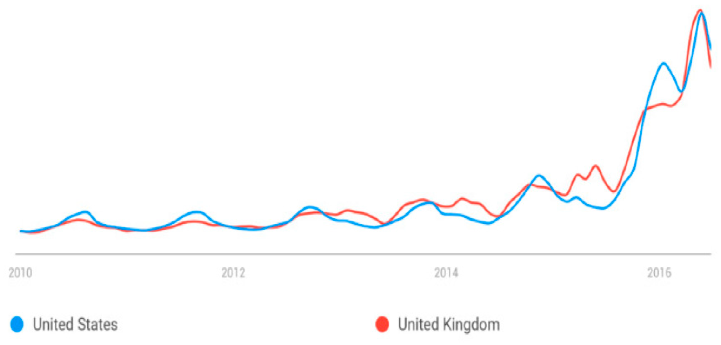
Boone (2016) asserts that Google Trends can also show which styles really catch on with shoppers when search patterns and geographic factors driving the biggest fashion trends in 2016 were analysed. For example, Figure 2 below shows Google Trends for bomber jackets which grew 297% YoY in the UK and 612% YoY in the US and illustrated the shift towards genderless fashion (Boone 2016). In addition, fashion companies can track Google searches to identify purchasing decisions and swiftly meet that demand (Hastreiter 2016). Given the increasing competition within the industry, such analytics can give any brand or retailer a clear competitive advantage in terms of more efficient resource allocations and minimising waste.
There is also evidence of some fashion brands looking into exploiting Google Trends to their advantage for enhancing consumer engagement via improved online consumer experiences. One such example is Miinto, a leading Norwegian fashion retailer that created a fun nostalgia-based quiz using Google Trends to enable consumers to be fashion forward (Armstrong 2016). Google and Zalando teamed up to create Project Muze to exploit the data in Google’s Fashion Trends report using Neural Networks for creating designs based on users’ interests (Think with Google 2017). Whilst some have criticised the process (see for example, Perez (2016)), there is potential for further research and development to improve the outputs from such novel use of big data analytics.
The lack of academic research into Google Trends as a viable analytical tool for the fashion industry is indeed worrying for an industry which is valued at 3 trillion USD and 2% of the world’s GDP (Fashion United 2019). The relative neglect of Google Trends in the context of the fashion industry is surprising since research using Google Trends has increased dramatically in the last decade with lucrative applications in IT, communications, medicine, health, business and economics (Jun et al. 2018). It is our hope that the topics covered in this paper would motivate more academic research into fashion consumer Google Trends and its value for decision-making.

2.2. How Can Google Trends Help Strategic Fashion Management & Marketing Decisions?

In addition to presenting selected examples of how the fashion industry can benefit from analytics based on fashion consumer Google Trends for making more productive and strategic fashion management and marketing decisions, we also use this subsection to highlight the importance and utility of being able to forecast fashion consumer Google Trends accurately into the future.

2.2.1. Identifying Seasonal Patterns in Demand

The see-now, buy-now trend was expected to flatten out the seasonal peaks in the fashion industry via cruise collections and trans-seasonality. For example, in 2016, the luxury fashion house Burberry launched its entirely straight-to-consumer collection as it aimed to create a seasonless fashion calendar, breaking all the rules at the London Fashion Week (Brown 2016; Rodulfo 2016; Cusick 2016). However, evidence suggests that fashion remains highly seasonal (for example, the most recent retail sales patterns in UK, as visible via the Office for National Statistics too supports this view). This could partly be due to the see-now, buy-now trend failing to become an industry standard as some early adopters such as Tom Ford found it backfired, whilst the Kering Group has so far resisted the model (Reuters 2018). Smith (2018) found, from Edited asserts, that there is growing need to understand the shifting seasonality of apparel. Whilst there is a plethora of evidence in academia indicating the importance of seasonality in fashion demand (Nenni et al. 2013), Thomassey (2014) correctly notes that not all fashion products have a seasonal demand (as continuity lines have year-round demand). Nonetheless, a considerable number of items are impacted by seasonality and thus, seasonality should be incorporated into fashion forecasting systems.
To this end, fashion consumer Google Trends could indicate consumers’ seasonality in demand for any given product and clearly show changes in seasonal demand patterns. Figure 3 considers Google web search patterns for ‘bomber jackets’, which not only show that there is a seasonal demand, but also that the seasonal demand patterns have changed considerably over time. For example, there is a diminishing seasonal demand from 2004 up until December 2013, which is followed by the seasonal demand shifting upwards prior to illustrating a downward sloping trend as visible.
If a fashion company could find evidence of a significant positive correlation between its historical sales for a product and consumer interest in the said product, as indicated via fashion consumer Google Trends, then it is reasonable to assume that Google Trends could serve as a potential indicator for changes in future sales. It is noteworthy that Boone et al. (2017) found evidence of Google Trends improving sales forecasts. Therefore, it would be useful if fashion brands can accurately forecast future seasonality movements in fashion consumer Google Trends, enabling better decisions on what to stock, when to stock and how much to stock, in addition to using consumer trends to determine when to reduce and increase the price points from a marketing perspective. Hastreiter (2016) supports the view that tracking Google searches could be useful for identifying purchasing decisions and that acting upon such analytics to swiftly meet the growing demand could strengthen top lines through value realisation which enables removal of discount traps and more full price sales.
From this example, it is evident that the fashion industry could benefit through the application of statistical signal processing models which have the capability of extracting seasonal variations in data and providing insights and seasonal forecasts into the future. Moreover, the data in Figure 3 appears to be nonstationary over time and would therefore benefit from the application of nonparametric models, which do not assume stationarity.

2.2.2. Competitor Analysis

Gone are the days when luxury brands viewed online as a “mass market” (Deloitte 2018). With e-commerce expected to account for 36% of global fashion retail sales by 2020 (Meena 2018), all brands are focused on getting their digital footprint right. Moreover, recent reports indicate that consumers are increasingly choosing online shopping over the high street (BBC 2019). This preference is understandable as online shopping enables quick and easy price comparisons and ensures that physical journeys are not wasted, as retailers may not always carry full stock of sizes and colours in every store. As consumers demand better shopping experiences, luxury brands are exploiting the web to provide personalised shopping experiences (Deloitte 2018) with global investments in improving luxury online shopping now topping 1 billion USD (Gallhagher 2017). Fashion consumer Google Trends has the potential to help brands assess the success of their online marketing campaigns and enable identification of key competitors through brand search trend analysis (Willner 2017). In addition, analysts can also compare performance based on specific products.
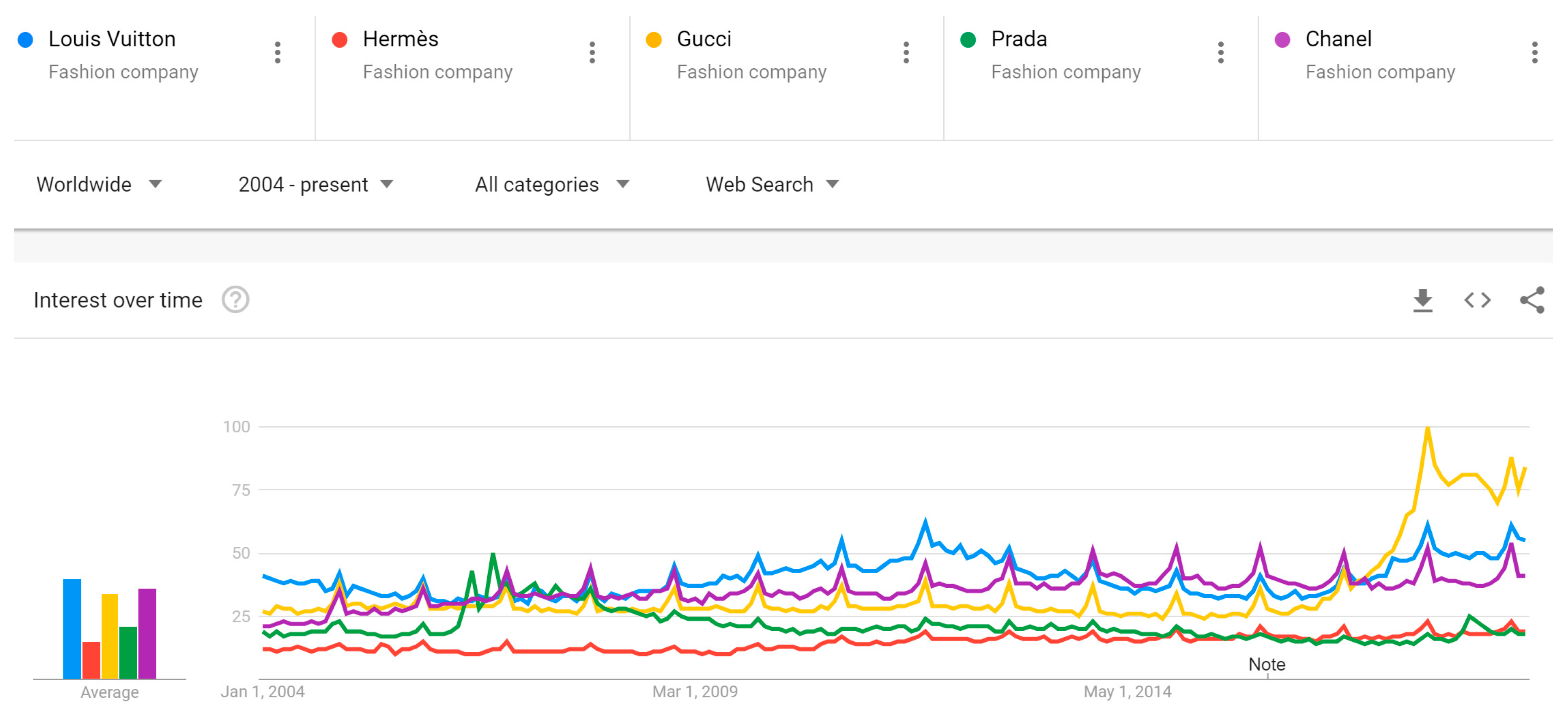
For example, Gucci was reported to be the most popular Google search for fashion brands in 2017 with Louis Vuitton coming in at number two (Bobila 2017), this trend appears to be continuing in 2019 (see, Figure 4). Such insights are useful for fashion brands as it shows them the effectiveness of their online marketing campaigns and websites in terms of engaging the consumer. In addition, brands can easily identify who their key competitors are, and this can enable them to study their competitors’ approaches to engaging the consumer online and improve upon their existing approaches. The simple example in Figure 4 also clearly illustrates how, except for Gucci, Louis Vuitton and Chanel, the other luxury brands considered here are struggling to get their online footprint set right. Interestingly, the trends shown here continue in terms of image, news, Google Shopping and YouTube searches online.
However, it is important to remember that high search trends are not always a good thing. It is imperative that managers and analysts understand the underlying cause of emerging trends (Bradlow et al. 2017). For example, Figure 5 below shows worldwide fashion consumer Google Trends for the search term “Dolce & Gabbana”. The peak popularity for the fashion brand in November 2018 is far from positive as this coincides with its disastrous marketing campaign featuring a Chinese woman struggling to eat pizza and other Italian foods with chopsticks (Hall and Suen 2018). Therefore, it is advisable that peaks in Google Trends are always cross-checked with research into other information surrounding brands to ensure it is a positive gain as opposed to one which is fuelled by negative media.
Such in-depth analysis of fashion consumer Google Trends data is useful for forecasting models looking at predicting the future of competition based on historical data. This is because outliers could be removed via time series analysis models which enable denoising; this would ensure the forecasts being generated are more realistic and accounts for negative press. Those interested in an example of a denoised time series whereby signal processing was used to remove an outlier are referred to Hassani et al. (2018, Figure 5).

2.2.3. Identifying Brand Extension Opportunities

Brand extension, a popular and fundamental luxury brand marketing strategy (Eren-Erdogmus et al. 2018) refers to the launching of a new product under an existing brand name. Investing in new products within the fashion industry can be a costly affair. Fashion brands now have the option of analysing fashion consumer Google Trends for the products/sectors they plan on expanding into, to understand the consumer demand/sentiment towards the said product or sector. For example, Figure 6 below shows fashion consumer Google Trends for smart watches. It is evident that the consumer interest in smart watches is increasing over time and is also becoming more seasonal in demand. Such information can give confidence to decision makers about investing in new products and show the best period for launching said investments in their brands.
Solanki (2018) discusses the importance of plus-size as a growing fashion sector, and notes how Google Trends not only shows an increasing number of searches, but also that the term reached its peak popularity in UK in June 2018. Another example is presented by Young (2018) with regard to the future of vegan fashion; she discusses Google Trends as a tool which can indicate the future for this particular sector. Overall, it is evident that the ability to accurately forecast such trends into the future based on historical fashion consumer Google Trends data can be of utmost importance for fashion brands to develop better and more successful brand extension strategies.

2.2.4. Identifying Better Marketing Terms

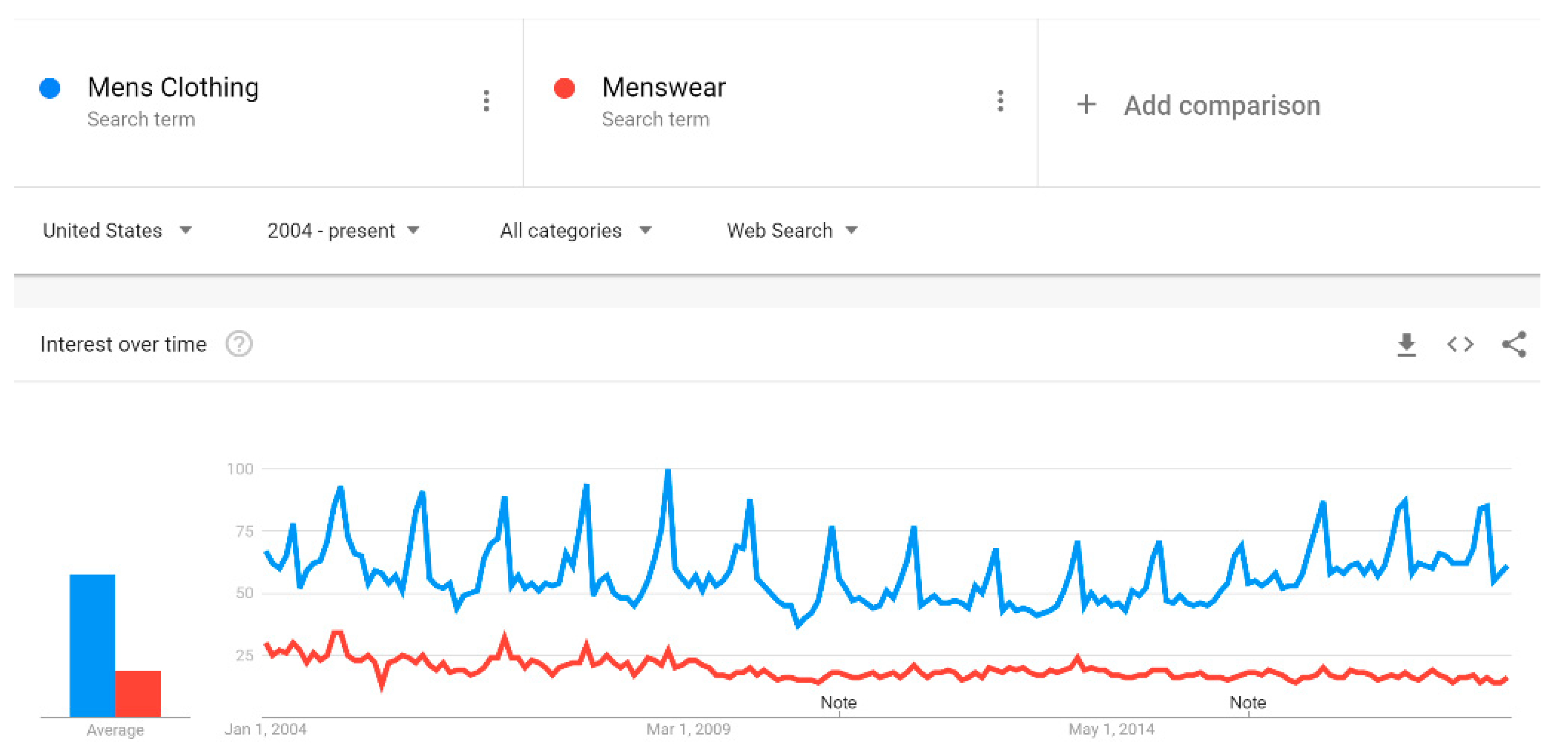
Fashion marketing and advertising are more complex today than ever before, with consumers demanding ethical advertising and use of appropriate language (Bae et al. 2015). As Forni (2018) asserts, when marketing fashion online, the failure to understand the need for geographical language changes can be detrimental. Fashion consumer Google Trends can help fashion brands ensure they are using the most appropriate terms online for marketing and search engine optimisation in the countries in which they operate. For example, Figure 7 below shows the fashion consumer Google Trends for two product categories in two different markets (i.e., United States and United Kingdom). This example illustrates that using the term ‘Men’s Clothing’ as opposed to ‘Menswear’ on a brand’s websites or even offline marketing campaigns is likely to attract more engagement from the consumer in the United States. On the other hand, it also shows that using the term ‘Men’s Clothing’ in the United Kingdom market will have a completely different effect as the term ‘Menswear’ is more popular. The ability to analyse fashion consumer Google Trends by country adds more value as it enables brands to personalise their websites according to the consumer search interests in any given country across the globe. Once again, being able to forecast these fashion consumer Google Trends accurately into the future can help improve search engine optimisation for fashion brands.

3. Data

Burberry Google Trends

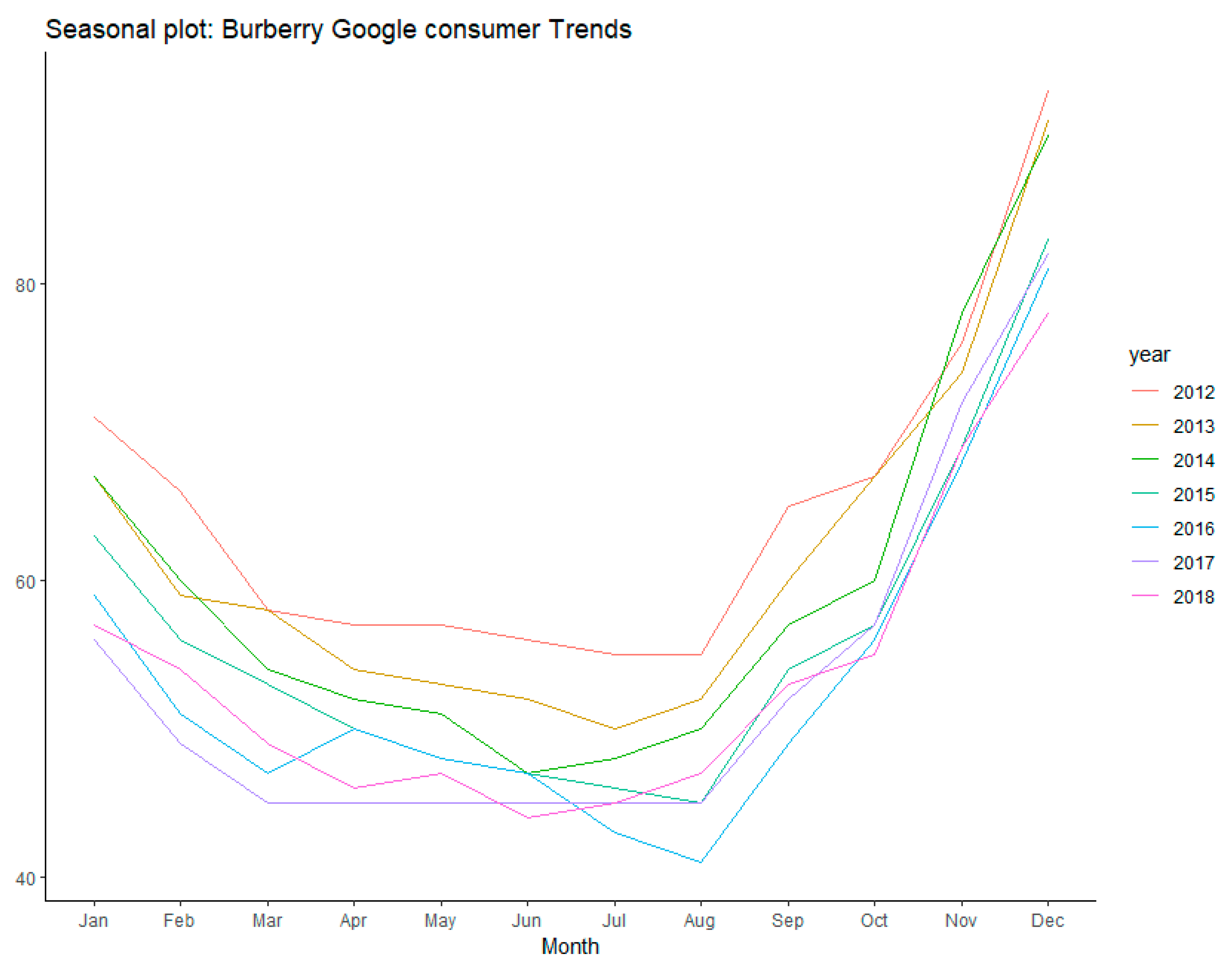
The choice of Burberry as the data set of interest for this study was influenced by several factors. First, Burberry is one of the UK’s highest profile exporters, but supply chain disruptions resulting from Brexit are expected to add millions in extra trade costs for this fashion house (Rovnick 2019). Accordingly, there is a need for more data analytics into this brand to help improve its profitability via more lucrative resource allocations. Secondly, as evidenced in the seasonal plot in Figure 8, Burberry appears to be struggling in terms of increasing and maintaining online consumer interest in the brand name. Thus, there is need for further analysis and forecasting of future online behavioural trends for Burberry so that the management can put in place a series of actions for improving its online footprint and be better positioned to compete with other luxury fashion brands. Thirdly, Burberry believes in the importance of digital innovation and sees ‘online’ as the first access point to its brand (Burberry 2018a). Therefore, Google Trends-based analytics has the potential to help the brand ensure its online content remains highly relevant to its consumers. For example, Burberry (2018a) states the brand wishes to personalise online homepages, and fashion consumer Google Trends-based analytics can help the brand in identifying the most popular product categories and terminology for any given market (see Section 2.2.4). Fourthly, as a brand, Burberry has recently demonstrated its willingness to change for the better and become more sustainable. For example, in July 2018 Burberry was called out for burning millions of its products to protect its brand (BBC 2018). Swift to act, by September 2018 Burberry announced that it will stop the practice of destroying unsaleable products and the use of real fur, and work towards reusing, repairing, donating or recycling their unsaleable goods (Burberry 2018b; Hanbury 2018; Bain 2018). Thus, Burberry is a brand to watch, and is a brand that is responsive to the consumers’ needs and wants.
The data considered within the forecast evaluation was extracted through Google Trends and relates to monthly web search history for the search term “Burberry” as recorded worldwide from January 2004–February 2019. The chosen time period is influenced by the availability of data and the fact that longer time horizons can capture the historical trends and changes in seasonal variations visible in time series. Analysing such detailed information should enable forecasting models to generate more accurate parameters for modelling and forecasting future consumer trends. However, it should be noted that depending on the objective of the forecasting exercise, the use of shorter time series can be more useful under certain scenarios. For example, if a fashion company does not wish to rely on a nonparametric forecasting model, then analysing shorter time series can be a better option as longer time series are more likely to be nonstationary over time (Bradlow et al. 2017).
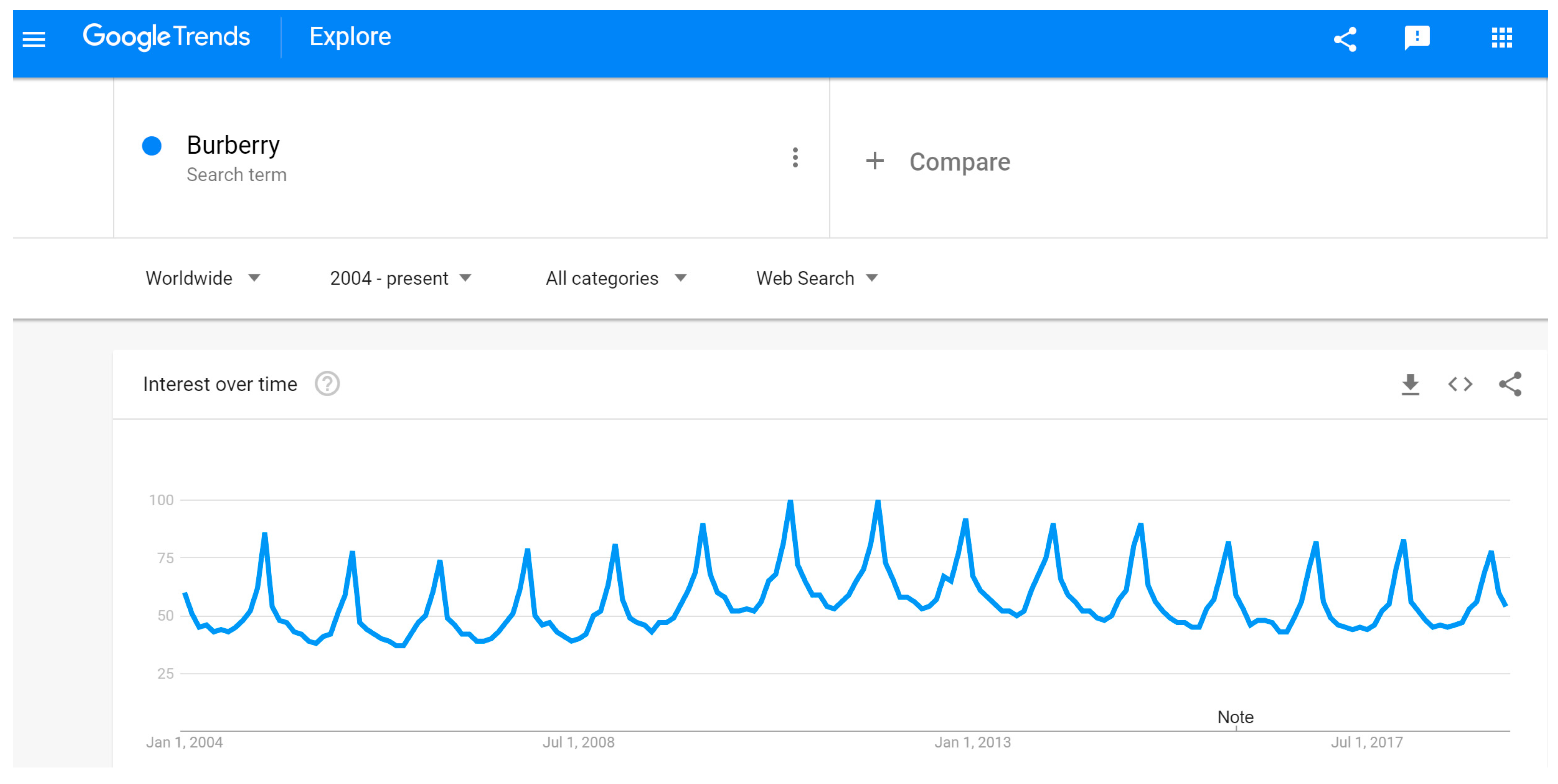
Figure 9 shows the time series plot for Burberry’s fashion consumer Google Trends. The peak in consumer trends has remained constant over time and occurs in December annualy coinciding with Christmas, but interestingly, consumer interest in the brand always declines during the start of the new year. We also plot the seasonal changes in consumer trends over the last seven years as an example (Figure 8). This shows how consumer interest in Burberry has declined each season as recorded via Google Trends (with the exception of 2018 which is slightly better than 2017). Moreover, upon closer inspection, it is evident that there are constant shifts in seasonality in terms of Burberry’s fashion consumer Google Trends over time. For example, the occurrence of troughs vary between June, July and August resulting in varying amplitudes. It will be interesting to see how the forecasting models perform at capturing these minute, yet very important changes.
As visible (Figure 9), the data is highly seasonal yet fairly stationary (there was no evidence of seasonal unit roots based on the Osborn–Chui–Smith–Birchenhall (Osborn et al. 1988) test for seasonal unit roots) over this time period. In terms of the vertical axis in Figure 9 and the figures that follow, the numbers shown represent search interest relative to the highest point on the chart for the given region and time. A value of 100 is the peak popularity for the term. A value of 50 means that the term is half as popular. A score of 0 means there was not enough data for this term.

4. Forecasting Models

At the outset, it is noteworthy that the forecasting exercise is recursive (i.e., within each horizon of interest, the models re-estimate parameters by remodelling the historical data with each new observation that is introduced). This process continues until all required forecasts are computed) and considers horizons of 1, 3, 6 and 12 months ahead. At each horizon, we compute Nh + 1 forecasts, where N = 60, and h refers to the forecasting horizon of interest. The accuracy of the out-of-sample forecasts are evaluated via the Root Mean Squared Error (RMSE) and Ratio of the RMSE (RRMSE) criteria. Those interested in the formulae for the RMSE and RRMSE are referred to Silva et al. (2019) and references therein. In what follows, we provide concise introductions to the forecasting models used in this paper.

4.1. Autoregressive Integrated Moving Average (ARIMA)

The Box and Jenkins (1970) ARIMA model is one of the most popular and frequently used parametric time series analysis and forecasting models (Silva et al. 2019). As a parametric model, ARIMA is bound by the assumptions of normality and stationarity of the residuals and linearity. Whilst such assumptions are unlikely to hold in the real world, for univariate forecast evaluations, it is widely accepted that ARIMA should be considered as a benchmark forecasting model (Hyndman 2010). Moreover, ARIMA has previously been adopted in studies looking at forecasting variables of interest in the fashion industry, for example, Wong and Guo (2010), Yu et al. (2012) and Liu et al. (2013). However, in contrast to the aforementioned papers, here, we rely on an automated and optimised algorithm for ARIMA, which is popularly referred to as ‘auto.arima’, and is accessible freely via the forecast package in R. Those interested in details of the theory underlying ‘auto.arima’ are referred to Hyndman and Athanasopoulos (2018).

4.2. Exponential Smoothing (ETS)

In brief, ETS forecasts are weighted averages of past observations, where a higher weight is assigned to the more recent record with overall exponentially decaying weights (Hyndman and Athanasopoulos 2018). The development of the ETS technique is closely associated with the work of Brown (1959), Holt (1957) and Winters (1960), whilst its performance in a fashion context was previously evaluated through the work of Fumi et al. (2013). In this paper, we rely on the nonparametric, automated ETS algorithm found within the forecast package in R. Instead of replicating information surrounding the 30 ETS formulae evaluated as part of the modelling process, we refer those interested in details of the theory underlying ETS to Hyndman and Athanasopoulos (2018).

4.3. Trigonometric Box–Cox ARMA Trend Seasonal Model

The TBATS model was developed by De Livera et al. (2011) for handling complex seasonal patterns. Given the earlier discussion around the importance of seasonality in fashion, it is useful to evaluate the performance of this model at forecasting fashion consumer Google Trends. Also noteworthy is that this application is the initial application of TBATS for forecasting in fashion. In brief, TBATS is an exponential smoothing state space model with Box–Cox transformation, ARMA error correction and Trend and Seasonal components, for which the detailed theoretical foundation can be found in Hyndman and Athanasopoulos (2018). Once again, we rely on the automated TBATS algorithm provided via the forecast package in R.

4.4. Neural Network Autoregression (NNAR)

Neural networks represent a nonparametric forecasting model made available as an automated algorithm via the forecast package in R. The feed-forward neural network model with one hidden layer is denoted by NNAR (p, P, k)m, where p refers to lagged inputs, P takes a default value of 1 for seasonal data (as is the case here), k refers to nodes in the hidden layer and m refers to a monthly frequency. Those interested in the theory are referred to Hyndman and Athanasopoulos (2018), whilst a discussion around the impact of seasonality on neural network forecasts can be found in Silva et al. (2019). Interestingly, there have been several applications of varying Neural Network models for forecasting in fashion research (Au et al. 2008; Sun et al. 2008; Yu et al. 2011; Xia et al. 2012; Kong et al. 2014).

4.5. Denoised Neural Network Autoregression (DNNAR)

The DNNAR model was introduced in Silva et al. (2019) as a solution to the issues identified with the NNAR model when faced with seasonal time series. In brief, the DNNAR model is a nonparametric hybrid model which combines the denoising capabilities of singular spectrum analysis (Sanei and Hassani 2015) with the power of NNAR forecasting to produce superior forecasts. This paper marks the introductory application of the DNNAR model as a useful and viable option for forecasting in the fashion industry. We believe the application of the DNNAR model can be useful in this context because, as Choi and Varian (2012) asserts, the sampling method used to calculate Google Trends varies somewhat from day-to-day, thus creating a sampling error which contributes to additional noise in the data. Given that noise refers to random components which cannot be forecasted, it makes sense to reduce noise levels in fashion consumer Google Trends via the use of a denoising algorithm.

5. Empirical Results

In this section, we present the findings from our attempts at forecasting fashion consumer Google Trends using a variety of univariate time series analysis and forecasting models. Table 1 below reports the out-of-sample forecasting results from the forecasting exercise. The first observation is that there is no single model that can forecast fashion consumer Google Trends for “Burberry” best across all horizons. We find forecasts from ARIMA outperforming all competing models at h = 1 month-ahead, whilst forecasts from the TBATS model outperforms the competing forecasts at h = 3 months-ahead. In the long run, i.e., h = 6 and 12 months-ahead, we find ETS forecasts to be more accurate than those from ARIMA, TBATS and NNAR models.
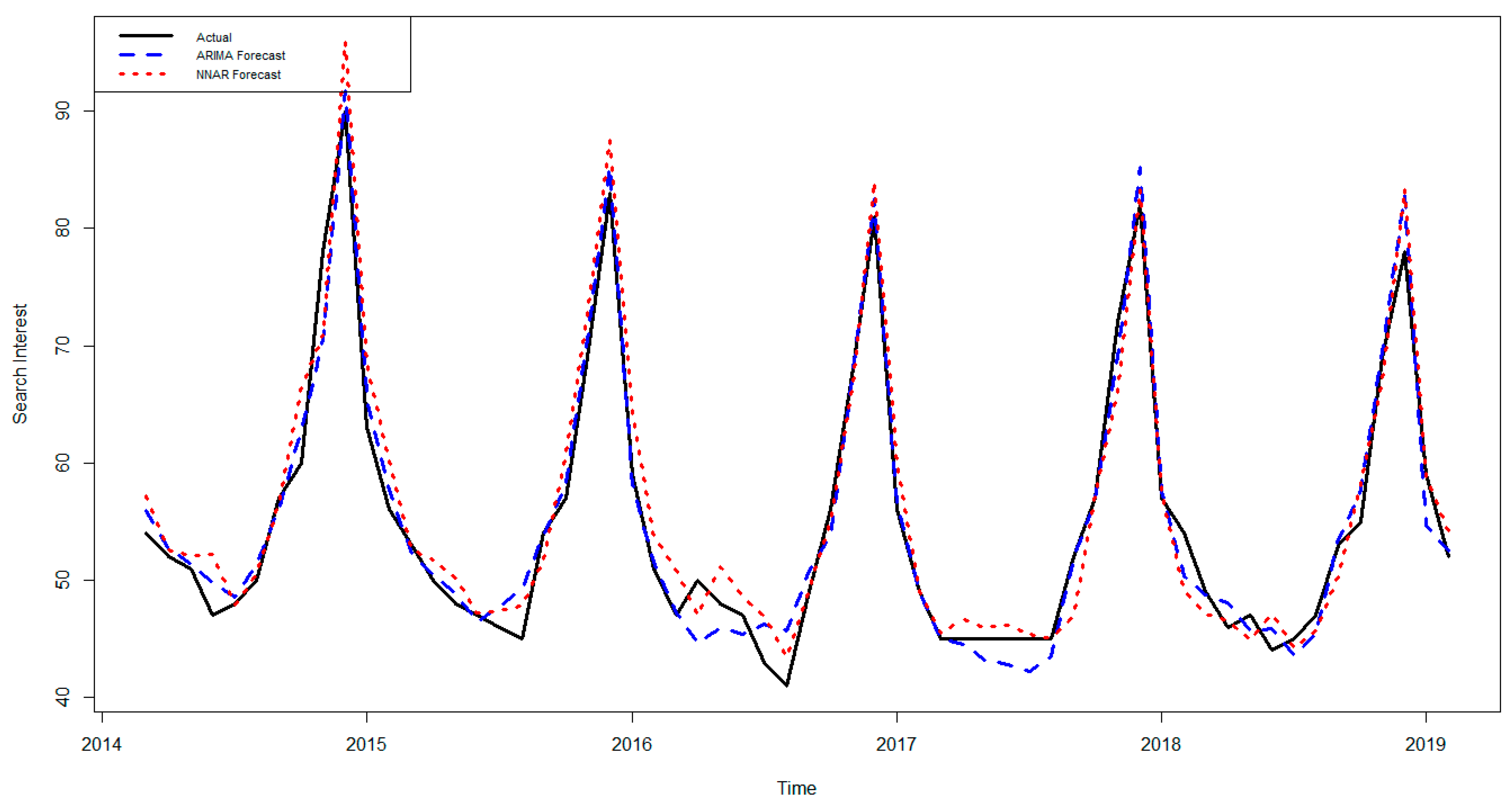
The NNAR model is seen to be the worst performer at forecasting fashion consumer Google Trends for “Burberry” across all horizons. Figure 10 shows a time series plot of the best and worst performing forecasts at h = 1 month-ahead. In relation to the ARIMA model, the NNAR model fails at forecasting the peaks in search trends accurately (in addition to the problems with forecasting troughs accurately). Therefore, these initial findings indicate that if a fashion company wishes to forecast fashion consumer Google Trends for “Burberry” using univariate models, then they would have to switch between models depending on the forecasting horizon of interest. From an operational perspective this is problematic as one would prefer to adopt a single model for forecasting across all horizons so that it gives more consistency. As such, we extend the modelling process further in search of a univariate model which can provide consistently accurate forecasting results across all horizons.
Even though the NNAR model was the worst performer for this data, we find it pertinent to give it further consideration; especially as in an era of big data the importance of data mining techniques such as neural networks for the future of fashion analytics should not be ignored. Moreover, existing fashion trend forecasting platforms, such as Edited (2019), also overly rely on neural network-based models for its data analytics. Accordingly, we call upon a recently published hybrid neural network model which is referred to as the DNNAR model (Silva et al. 2019).
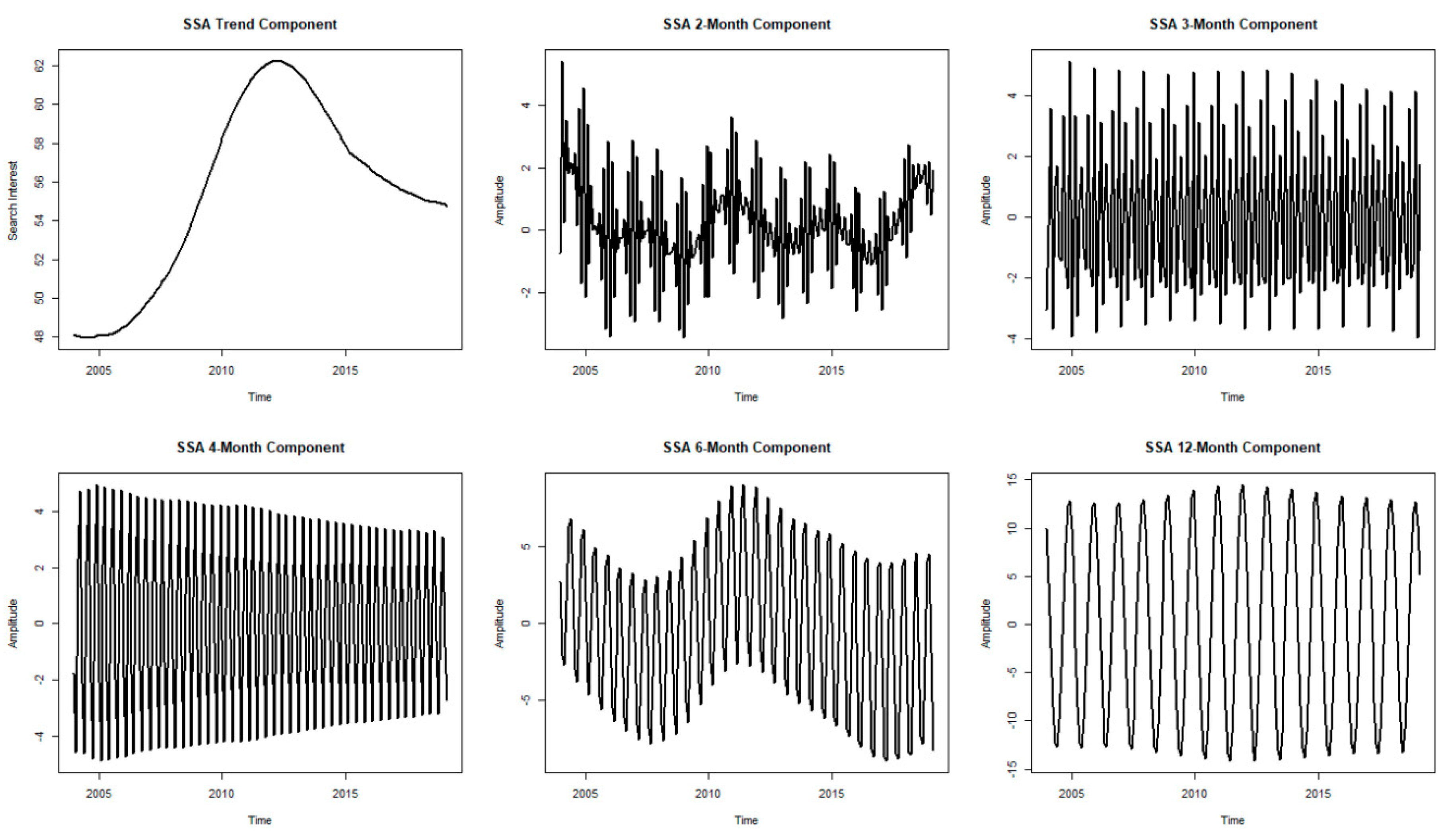
The first step of the DNNAR model involves the application of SSA for denoising the “Burberry” fashion consumer Google Trends series and extracting signals to create a less noisy, reconstructed series. This reconstructed series is then used as input data for generating NNAR forecasts—in a nutshell this summarises the DNNAR model. Figure 11 below shows the SSA signal extractions. The extracted components themselves will relate to a trend, periodic components, quasi-periodic components and noise (Hassani et al. 2016b). The combination of these signals provides us with the reconstructed, smoothed “Burberry” fashion consumer Google Trends series for forecasting with NNAR.
The trend extraction in Figure 9 shows the long run behaviour of online consumer trends for “Burberry”. Accordingly, it indicates the necessity for rethinking Burberry’s online marketing strategies as following the peak in March 2012, online consumer interest in the brand indicates an ongoing declining trend over time. The upward sloping trend between 2005 and 2012 is attributable to Burberry’s successful initiatives in driving online consumer interest in the brand through launching its UK transactional website in 2006, to the first ever live-streamed Burberry fashion show in 2009, to launching Burberry.com in 2011 (Burberry 2019). In terms of seasonality, Figure 11 also clearly indicates that Burberry’s fashion consumer Google Trends are strongly influenced by seasonal factors. Moreover, the seasonality underlying this time series is of varying amplitude depending on the periodicity in question. These seasonal patterns add further to the difficulty associated with forecasting Burberry’s fashion consumer Google Trends. It is noteworthy that the use of SSA for denoising fashion data also enables fashion companies to forecast seasonal variations alone to determine how consumer trends can vary over selected periodic cycles.
Table 2 below reports the out-of-sample forecasting RRMSEs for “Burberry” fashion consumer Google Trends. Here, we consider the DNNAR model as the benchmark and report all results relative to same. As such, where the RRMSE is less than 1, it indicates the DNNAR model is more accurate than a competing model. Moreover, the RRMSE criterion enables us to quantify the accuracy gain further as a percentage, such that it equals 1-RRMSE%. First and foremost, it is evident that the DNNAR model outperforms ARIMA, ETS, TBATS and NNAR forecasts for “Burberry” fashion consumer Google Trends and takes over as the best univariate forecasting model across all horizons. In addition, the majority of the RRMSEs reported here represent statistically significant differences between forecasts (except in the very long run at h = 12 months-ahead).
The results in Table 2 show that when forecasting at h = 1 month-ahead, DNNAR forecasts are significantly better than forecasts from ARIMA, ETS, TBATS and NNAR models by 28%, 35%, 32% and 47%, respectively. Likewise, at h = 3 months-ahead, the DNNAR forecasts are 29%, 33%, 29% and 53% significantly better than ARIMA, ETS, TBATS and NNAR forecasts, respectively. At h = 6 months-ahead, the DDNAR model outperforms the competing forecasts with statistically significant accuracy gains of 27%, 27%, 29% and 46%, respectively. Finally, at h = 12 months-ahead, the DNNAR model outperforms all competing models but we fail to find evidence of statistically significant differences between forecasts, suggesting that these long-term forecasting gains could be a result of chance occurrences.
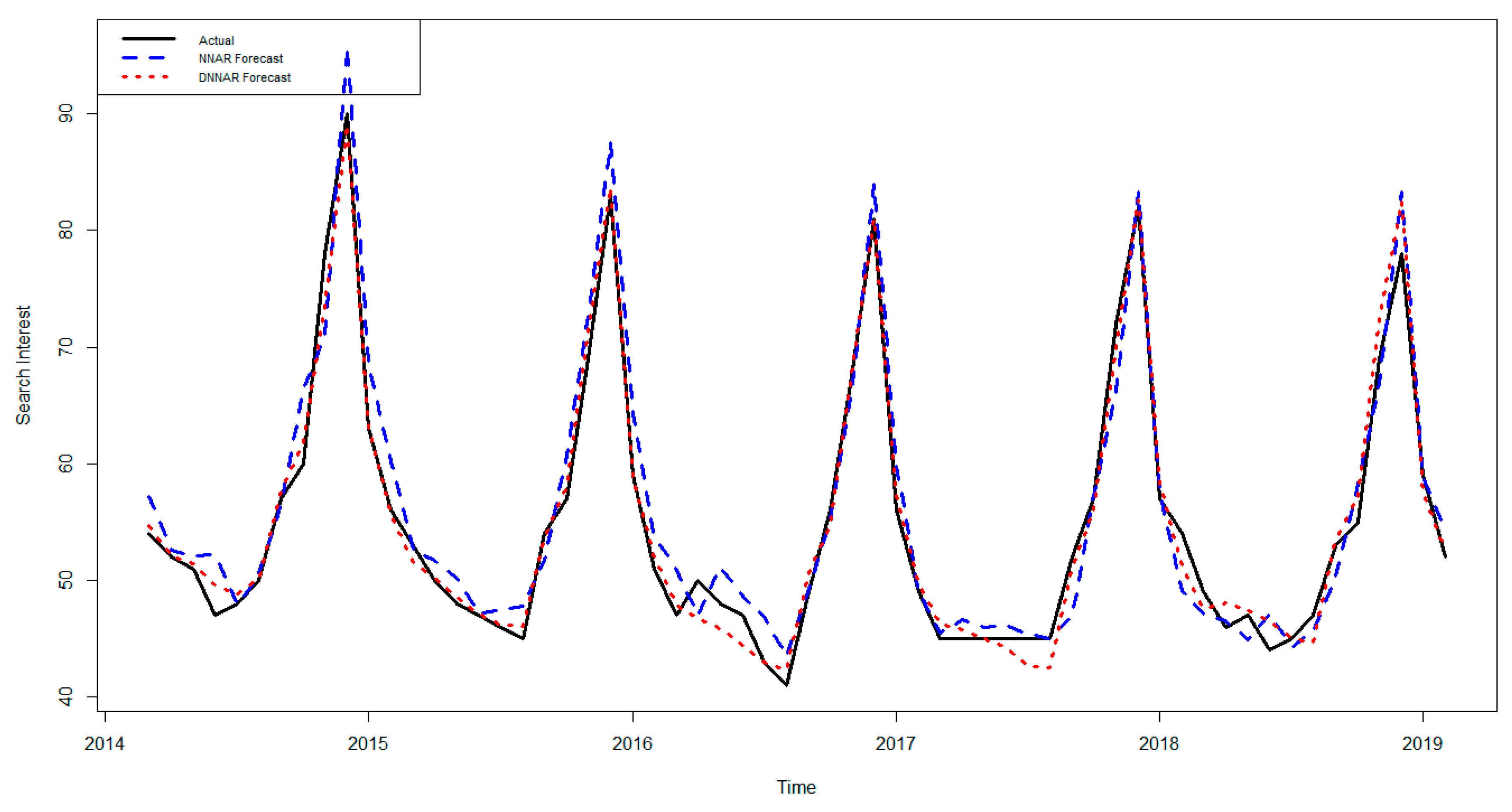
Finally, Figure 12 provides a graphical representation of the out-of-sample forecasts at h = 1 month-ahead from the DNNAR and NNAR models. Upon close inspection, it is visible that denoising with SSA has enabled the DNNAR model to accurately forecast 4/5 peaks in the out-of-sample data, whilst also providing comparatively better forecasts for 4/5 troughs in relation to the NNAR model. Forecasting Burberry’s fashion consumer Google Trends with DNNAR can enable the prediction of change points in consumer trends more accurately, and strategists can then make use of this information to inform their resource allocations and decision-making. For example, more efficient decisions on when to start targeting online marketing campaigns to uplift consumer interest in the brand and vice versa could be made well in advance. The ability to forecast when consumer trends would rise and fall, and the time period over which a contraction could last, or a recovery could take can be of utmost importance for strategic fashion management and marketing decision-making.

6. Discussion

We begin our discussion with a comparison of our findings with those from previous research. As Nenni et al. (2013) note, the importance of seasonality in fashion demand continues to be visible within Burberry’s fashion consumer Google Trends, whilst the seasonal plot in Figure 8 further evidences Smith’s (2018) assertion that there is a growing need to understand the shifting seasonality in fashion products.
Overall, the forecast evaluation undertaken in this study saw the introduction of several new time series analysis models for forecasting fashion data and this combination of new methods applied to new data has resulted in new research insights as suggested by Bradlow et al. (2017). First and foremost, in line with Jun et al.’s (2018) assertion that the purpose of big data utilisation shifting from monitoring to forecasting, our forecasting evaluation of fashion consumer Google Trends illustrates the possibility of accurately forecasting fashion consumer Google Trends using time series analysis models. Secondly, we evidence how Hassani and Silva’s (2015) assertion that noise reduction is important for big data forecasting is reasonable and extremely useful in helping generate forecasts, which are more consistent in accuracy across both short and long run horizons.
The introductory application of the DNNAR model for fashion forecasting yields similar findings to those reported in Silva et al. (2019) where the authors found the DNNAR model providing significantly better forecasts when faced with highly seasonal data. We also extend the comparison of the DNNAR model’s performance to include the TBATS model in addition to the ARIMA and ETS models which were considered in Silva et al. (2019). The findings here indicate that forecasts from the DNNAR model can outperform those from the TBATS model too.
Finally, as this is the first attempt at forecasting fashion consumer Google Trends, we are unable to compare our findings with directly comparable studies. Nevertheless, the superior forecasting performance of the DNNAR model is in line with the findings in Yu et al. (2012), where the authors found that artificial neural network models outperformed ARIMA at forecasting fashion colour trends; Wong and Guo (2010) found neural network forecasts outperformed ARIMA in terms of forecasting fashion retail supply chains. Au et al. (2008) found neural networks to be a good forecasting model for fashion retail data with weak seasonal trends. In contrast, our findings show that the DNNAR model which denoises seasonal data can produce significantly better forecasts for highly seasonal fashion data.

6.1. Are Web Searches for Burberry Predominantly Generated by Online Fashion Consumers who are Looking to Shop?

The simple answer is that we do not know for certain. Such analysis would require access to microlevel data around Burberry’s monthly sales (both online and offline) which could then be evaluated in detail via causality tests. However, it is important to remember that fashion brands load millions of Stock Keeping Units (SKUs) relating to different sizes and different colour ways online regardless of whether consumers buy or not. As such, Google Trends can still be useful for brands to identify the consumer attitudes towards its product range, and to identify which SKUs are most popular online (regardless of whether these trends translate into sales or not). The ensuing analytics can ensure brands are providing the options demanded by their consumer and if brands can accurately predict future consumer trends about these SKUs, then they can make more efficient managerial and marketing decisions leading to better resource allocation.
Nonetheless, Google Trends also report Google Search patterns from consumers accessing Google Shopping. We analysed “Burberry” web search patterns and Google shopping patterns. Figure 13 shows the time series and scatterplots used at the beginning of this analysis. As both graphs indicated the possibility of a strong correlation, we evaluated for same via Pearson’s correlation and found a statistically significant strong, positive, linear correlation of 72% between web search patterns and Google shopping patterns for the search term “Burberry”. Whilst appreciating that correlation does not imply causation, these findings indicate that a 72% increase in web search patterns can signify a 72% increase in Google shopping patterns related to “Burberry”. This justifies the consideration of web searches as a proxy for online consumer shopping behaviour to a certain extent and appears to be in line with Hastreiter (2016) and Boone et al. (2017) assertions that Google Trends can identify purchase decisions. Moreover, Bloomberg (2017) reported that Google Trends was able to predict a slowdown in Salvatore Ferragamo SpA sales six to nine months before it happened in 2015, and that Prada reports one of the highest correlations between Google web searches and revenue growth.

6.2. Google Trends vs. Trend Forecasting Giants (Edited & WGSN)

To the best of our knowledge, Edited does not exploit Google Trends data to inform its current analytics and there is no publicly available information which indicates same. Accordingly, first and foremost, in contrast to the analytics made possible via Edited, Google Trends can help users determine the effectiveness of marketing campaigns from a very broad sense (as explained in detail in Section 2.2). Secondly, Edited and WGSN are both subscription-based services that are purely focused on product listings, and therefore fail to provide a complete picture, whereas Google Trends is entirely free to access and can be utilised to analyse online consumer interest on any aspect of fashion.
Thirdly, it is not possible to export raw data from Edited (unless you pay for subscription), which hinders the ability to conduct independent, raw analysis using new methods, and could potentially hinder the discovery of new research insights (Bradlow et al. 2017). In contrast, users can freely download the aggregated data capturing online fashion consumer Google Trends over time. In addition, the founder of WGSN states that consumers complain about everything looking the same today, but that it is inevitable as thousands of fashion companies are signed up for trend forecasting services and looking at the same colour, material and silhouette forecasts (The Fashion Law 2017). Thus, there is the question of a decline in creativity which is the backbone of fashion. It is our notion that the inclusion and consideration of fashion consumer Google Trends can add more variety to the eventual product offering.
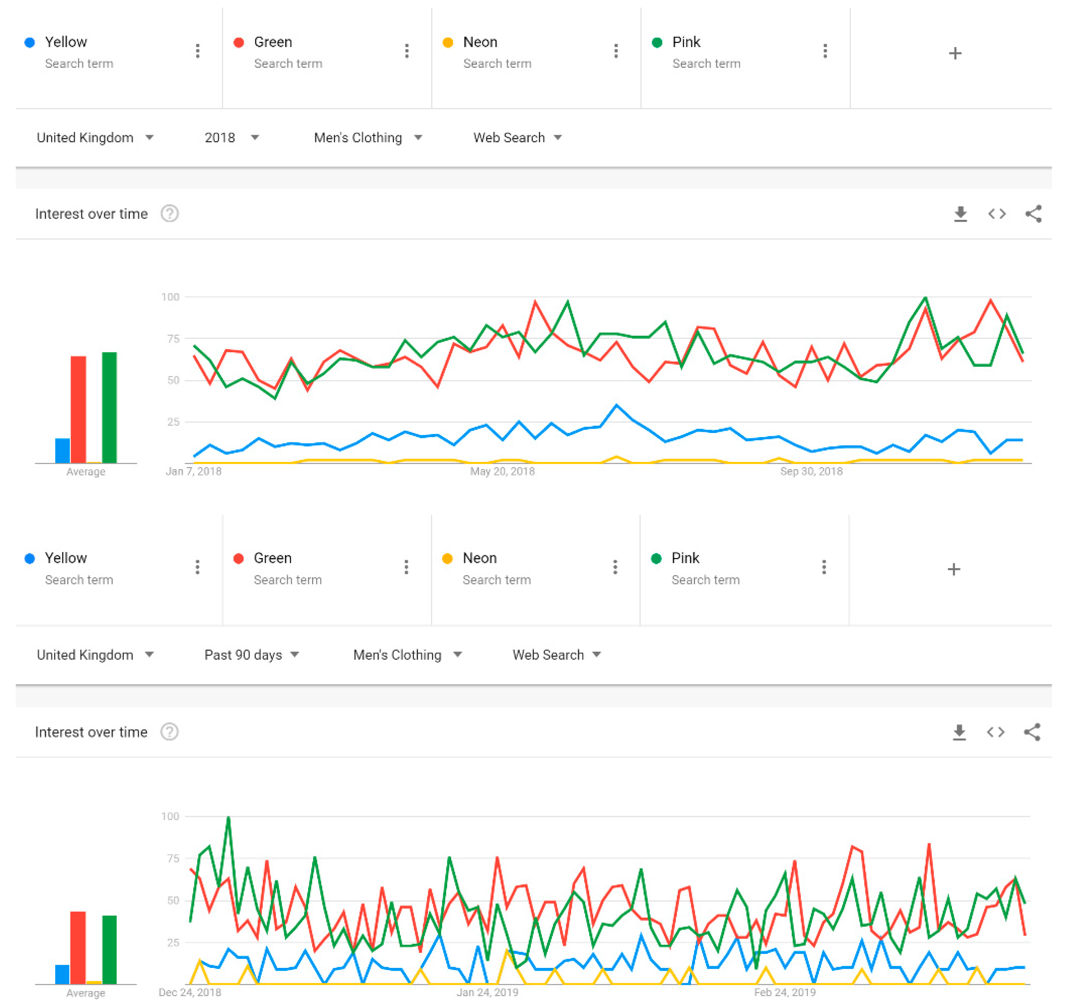
Finally, Edited mines the websites of brands and retailers around the globe and generates trends based on the patterns it identifies within the existing product offering (i.e., what is being stocked and what is sold). In contrast, Google Trends focus on consumer search interest and can offer insights which are more directly comparable with consumer needs and wants. For example, Edited predicts that in terms of colour ways; yellow, green, pink and neon would be the trending colour options for men’s clothing in 2019 (Yau 2019). However, if the trend forecasts also considered fashion consumer Google Trends, then it might have given a different and more relevant colour way forecast for 2019. Figure 14 below shows that even in 2018 yellow and pink were not popular colours in relation to men’s clothing web searches whilst the fashion consumer Google Trends for these colours in 2019 follows a similar trend. If Edited considered correlating their trends with fashion consumer Google Trends and forecasting same into the future, then they would be able to incorporate this new information into their decision models and improve the accuracy of their trend forecasts further. As such, we believe there is scope for the development of more efficient fashion trend forecasts by combining fashion consumer Google Trends data with the trend forecasts from Edited and WGSN.

7. Conclusions

In terms of the uses of Google Trends in fashion, we find evidence of the fashion industry seeking to exploit Google Trends to benefit the consumer experience. However, there is little evidence (and none from an academic perspective) of its exploitation as an analytical tool for better decision-making and forecasting in fashion. We present examples of how fashion consumer Google Trends can be useful for fashion brands to identify seasonal patterns in demand, conduct competitor analysis, brand extension opportunities and better marketing terms.
Regarding the overarching aim of this paper to determine the existence of a single univariate forecasting model that can predict fashion consumer Google Trends accurately across all horizons, using Burberry as an example, the forecast evaluation failed to find a single univariate model which could provide the best forecast across all horizons. The study considered both parametric and nonparametric forecasting models such as ARIMA, ETS, TBATS and NNAR. Whilst ARIMA, ETS and TBATS were successful in providing the best forecast at least at one horizon of interest, the NNAR model was the worst performer. The failure of any single model at providing the best forecast across all horizons could be a result of the complex seasonal variations with varying amplitudes underlying the Burberry fashion consumer Google Trends series.
Given that existing trend forecasting platforms such as Edited too relies on Neural Networks for its modelling and forecasts (Edited 2019), we were motivated to evaluate the performance of the DNNAR model when applied to a fashion context. Overall, this application resulted in providing overwhelming support indicating the importance of signal extraction and denoising for fashion analytics. This is because the application of the DNNAR model, which includes denoising and signal extraction with SSA prior to forecasting with NNAR, resulted in a model which was successful at providing the best forecast for Burberry’s fashion consumer Google Trends across all horizons with statistically significant outcomes in most cases. Thus, in addition to identifying a hybrid univariate model which can be used by Burberry for forecasting its fashion consumer Google Trends across all horizons, we also show the usefulness of applying denoising and signal extraction techniques for fashion data analytics in an era of big data.
Like all research, our study and its findings are not without its limitations. As discussed previously in our paper, it is well documented that using only search information for analytics without complementing it with other sources of big data and news has its limitations (Jun et al. 2018). Thus, brands should always consider using different types of information to support any strategic fashion management or marketing decisions they wish to pursue based on fashion consumer Google Trends. Moreover, in this paper, the DNNAR model is applied for forecasting a highly seasonal example of fashion consumer Google Trends. It is likely that these results will not hold for fashion consumer Google Trends which do not display such high levels of seasonality.
Nevertheless, our study opens several research avenues. Firstly, there is a need for more research that can provide conclusive evidence on whether fashion consumer Google Trends can help predict fashion purchases. Such research would require the fashion industry to agree on liberalising its practices when it comes to making data available for research purposes. Secondly, a more thorough forecast evaluation which considers a wider range of univariate and multivariate models at predicting a range of fashion consumer Google Trends for a variety of brands at higher frequencies should be undertaken. Thirdly, it would be interesting to collaborate with Edited and/or WGSN to determine how their trend forecasts can be further improved upon by incorporating fashion consumer Google Trends whilst assessing the existence of any correlation or causality between Google Trends-based fashion forecasts and Edited/WGSN trend forecasts.

Author Contributions

Conceptualization, E.S.S.; Data curation, H.H.; Formal analysis, E.S.S. and H.H.; Resources, L.G.; Supervision, D.Ø.M.; Writing—original draft, D.Ø.M.

Funding

This research received no external funding.

Acknowledgments

We would like to thank two anonymous referees for many helpful comments. However, any remaining errors are solely ours.

Conflicts of Interest

The authors declare no conflicts of interest.

References

  1. Armstrong, Paul. 2016. Why Your Business Should Be Using Google Trends. Available online: https://www.forbes.com/sites/paularmstrongtech/2016/04/01/why-your-business-should-be-using-google-trends/#4495c66d8268 (accessed on 22 July 2018).
  2. Au, Kin-Fan, Tsan-Ming Choi, and Yong Yu. 2008. Fashion retail forecasting by evolutionary neural networks. International Journal of Production Economics 114: 615–30. [Google Scholar] [CrossRef]
  3. Bae, Su Yun, Nancy Rudd, and Anil Bilgihan. 2015. Offensive advertising in the fashion industry: Sexual objectification and ethical judgments of consumers. Journal of Global Fashion Marketing 6: 236–49. [Google Scholar] [CrossRef]
  4. Bain, Marc. 2016. Google Already Knows the Fashion Trends that Will Be Popular this Fall. Available online: https://qz.com/767643/google-already-knows-the-fashion-trends-thatll-be-popular-this-fall/ (accessed on 22 July 2018).
  5. Bain, Marc. 2018. Burberry Won’t Burn Unsold Goods Anymore, but What about the Brands that didn’t Get Caught? Available online: https://qz.com/quartzy/1381150/burberry-wont-burn-unsold-goods-anymore-but-what-about-everyone-else/ (accessed on 24 March 2019).
  6. Bangwayo-Skeete, Prosper F., and Ryan W. Skeete. 2015. Can Google data improve the forecasting performance of tourist arrivals? Mixed-data sampling approach. Tourism Management 46: 454–64. [Google Scholar] [CrossRef]
  7. BBC. 2018. Burberry Burns Bags, Clothes and Perfume Worth Millions. Available online: https://www.bbc.co.uk/news/business-44885983 (accessed on 11 March 2019).
  8. BBC. 2019. Boohoo Remains in Fashion as Sales Surge. Available online: https://www.bbc.co.uk/news/business-46874367 (accessed on 19 February 2019).
  9. Bloomberg. 2017. Google Searches Seen as Luxury Investors’ Must-Have Tool in Fashion. Available online: https://www.businessoffashion.com/articles/news-analysis/google-searches-seen-as-luxury-investors-must-have-tool-in-fashion (accessed on 17 March 2019).
  10. Bobila, Maria. 2017. Chinese Retail giant Alibaba Launches ‘Big Data Anti-Counterfeiting Alliance’ with Louis Vuitton, Swarovski and More. Available online: https://fashionista.com/2017/01/alibaba-anti-counterfeit-alliance (accessed on 3 February 2019).
  11. Boone, Torrence. 2016. Fashion Trends 2016: Google Data Shows What Shoppers Want. Available online: https://www.thinkwithgoogle.com/advertising-channels/search/fashion-trends-2016-google-data-consumer-insights/ (accessed on 14 February 2019).
  12. Boone, Tonya, Ram Ganeshan, Robert L. Hicks, and Nada R. Sanders. 2017. Can Google Trends Improve your Sales Forecast? Production and Operations Management 27: 1770–74. [Google Scholar] [CrossRef]
  13. Box, George Edward Pelham, and Gwilym Jenkins. 1970. Time Series Analysis: Forecasting and Control. San Francisco: Holden-Day. [Google Scholar]
  14. Bradlow, Eric Thomas, Manish Gangwar, Praveen Kopalle, and Sudhir Voleti. 2017. The Role of Big Data and Predictive Analytics in Retailing. Journal of Retailing 93: 79–95. [Google Scholar] [CrossRef] [Green Version]
  15. Broomhead, David S., and Gregory P. King. 1986a. Extracting qualitative dynamics from experimental data. Physica D: Nonlinear Phenomena 20: 217–36. [Google Scholar] [CrossRef]
  16. Broomhead, David S., and Gregory P. King. 1986b. On the qualitative analysis of experimental dynamical systems. In Nonlinear Phenomena and Chaos. Edited by Sarben Sarkar. Bristol: Adam Hilger, pp. 113–44. [Google Scholar]
  17. Brown, Robert Goodell. 1959. Statistical Forecasting for Inventory Control. New York City: McGraw/Hill. [Google Scholar]
  18. Brown, Indya. 2016. Watch Burberry’s First See-Now, Buy-Now Collection Live. Available online: https://www.thecut.com/2016/09/watch-burberrys-first-see-now-buy-now-collection-live.html (accessed on 11 March 2019).
  19. Bulut, Levent. 2018. Google Trends and the forecasting performance of exchange rate models. Journal of Forecasting 37: 303–15. [Google Scholar] [CrossRef]
  20. Burberry. 2018a. Strategic Report. Available online: https://www.burberryplc.com/content/dam/burberry/corporate/Investors/Results_Reports/2018/Burberry_AnnualReport_FY17-18.pdf (accessed on 11 March 2019).
  21. Burberry. 2018b. Burberry Ends Practice of Destroying Unsaleable Products. Available online: https://www.burberryplc.com/en/news-and-media/press-releases/corporate/2018/burberry-ends-practice-of-destroying-unsaleable-products.html (accessed on 11 March 2019).
  22. Burberry. 2019. History. Available online: https://www.burberryplc.com/en/company/history.html (accessed on 16 March 2019).
  23. Choi, Hyunyoung, and Hal Varian. 2012. Predicting the present with Google Trends. Economic Record 88: 2–9. [Google Scholar] [CrossRef]
  24. Cusick, Ashley. 2016. Burberry Breaks All the Rules at London Fashion Week. Available online: http://www.essentialjournal.co.uk/burberry-breaks-all-the-rules-at-london-fashion-week/ (accessed on 11 March 2019).
  25. D’Arpizio, Claudia, and Federica Levato. 2017. The Millennial State of Mind. Available online: https://farfetch.prezly.com/bain--company-media-pack (accessed on 11 March 2019).
  26. De Livera, Alysha M., Robin John Hyndman, and Ralph David Snyder. 2011. Forecasting time series with complex seasonal patterns using exponential smoothing. Journal of the American Statistical Association 106: 1513–27. [Google Scholar] [CrossRef]
  27. Deloitte. 2018. Global Powers of Luxury Goods 2018: Shaping the Future of the Luxury Industry. Available online: https://www2.deloitte.com/content/dam/Deloitte/global/Documents/Consumer-Business/cb-global-powers-luxury-goods-2018.pdf (accessed on 11 March 2019).
  28. Edited. 2019. More Data. With More Data Science Behind It. Available online: https://edited.com/data/ (accessed on 16 March 2019).
  29. Eren-Erdogmus, Irem, Ilker Akgun, and Esin Arda. 2018. Drivers of successful luxury fashion brand extensions: Cases of complement and transfer extensions. Journal of Fashion Marketing and Management: An International Journal 22: 476–93. [Google Scholar] [CrossRef]
  30. Fashion United. 2019. Global Fashion Industry Statistics—International Apparel. Available online: https://fashionunited.com/global-fashion-industry-statistics/ (accessed on 19 September 2019).
  31. Forni, Christine. 2018. Using Google Trends to Get an Edge in Digital Marketing. Available online: https://growthpilots.com/using-google-trends-edge-digital-marketing/ (accessed on 11 March 2019).
  32. Fumi, Andrea, Arianna Pepe, Laura Scarabotti, and Massimiliano M. Schiraldi. 2013. Fourier Analysis for Demand Forecasting in a Fashion Company. International Journal of Engineering Business Management 5: 1–10. [Google Scholar] [CrossRef]
  33. Gallhagher, Kevin. 2017. Luxury Fashion Brands Shift Budgets to Digital. Available online: https://www.businessinsider.com/luxury-fashion-brands-shift-budgets-to-digital-2017-6?r=US&IR=T (accessed on 11 March 2019).
  34. Google. 2019. How Trends Data is Adjusted. Available online: https://support.google.com/trends/answer/4365533?hl=en (accessed on 11 March 2019).
  35. Gordon, Steven. 2017. Google Trends: A Metric of Consumer Behavior. White Paper. Sphere Quantitative Insights. Available online: https://sphereqi.com/wp-content/uploads/2017/09/whitepaper-6-30-17-Using-Google-Trends.pdf?pdf=GoogleTrends-A-Metric-Of-Consumer-Behavior (accessed on 23 March 2019).
  36. Guzman, Giselle. 2011. Internet search behavior as an economic forecasting tool: The case of inflation expectations. Journal of Economic and Social Measurement 36: 119–67. [Google Scholar] [CrossRef]
  37. Hall, Casey, and Zoe Suen. 2018. Dolce & Gabbana China Show Cancelled Amid Racism Outcry. Available online: https://www.businessoffashion.com/articles/news-analysis/racism-accusations-force-dolce-gabbana-to-cancel-chinese-fashion-show (accessed on 11 March 2019).
  38. Hamid, Alain, and Moritz Heiden. 2015. Forecasting volatility with empirical similarity and Google Trends. Journal of Economic Behavior & Organization 117: 62–81. [Google Scholar]
  39. Hanbury, Mary. 2018. Burberry is Changing Its Policy of Burning Millions of Dollars of Unsold Goods after Backlash Erupts Online. Available online: https://www.businessinsider.com/burberry-responds-to-backlash-stops-burning-unsold-goods-2018-9?r=US&IR=T (accessed on 24 March 2019).
  40. Hand, Chris, and Guy Judge. 2011. Searching for the picture: Forecasting UK cinema admissions using Google Trends data. Applied Economics Letters 19: 1051–55. [Google Scholar] [CrossRef]
  41. Hassani, Hossein, and Emmanuel Sirimal Silva. 2015a. A Kolmogorov-Smirnov Based Test for Comparing the Predictive Accuracy of Two Sets of Forecasts. Econometrics 3: 590–609. [Google Scholar] [CrossRef]
  42. Hassani, Hossein, and Emmanuel Sirimal Silva. 2015b. Forecasting with Big Data: A Review. Annals of Data Science 2: 5–19. [Google Scholar] [CrossRef]
  43. Hassani, Hossein, and Emmanuel Sirimal Silva. 2018. Big Data: A big opportunity for the petroleum and petrochemical industry. OPEC Energy Review 42: 74–89. [Google Scholar] [CrossRef]
  44. Hassani, Hossein, Gilbert Saporta, and Emmanuel Sirimal Silva. 2014. Data Mining and Official Statistics: The Past, The Present and The Future. Big Data 2: 34–43. [Google Scholar] [CrossRef]
  45. Hassani, Hossein, Xu Huang, and Emmanuel Sirimal Silva. 2016a. A Review of Data Mining Applications in Crime. Statistical Analysis and Data Mining: The ASA Data Science Journal 9: 139–54. [Google Scholar] [CrossRef]
  46. Hassani, Hossein, Zara Ghodsi, Emmanuel Sirimal Silva, and Saeed Heravi. 2016b. From nature to maths: Improving forecasting performance in subspace-based methods using genetics Colonial Theory. Digital Signal Processing 51: 101–9. [Google Scholar] [CrossRef]
  47. Hassani, Hossein, Xu Huang, and Emmanuel Sirimal Silva. 2018. Banking with blockchain-ed big data. Journal of Management Analytics 5: 256–75. [Google Scholar] [CrossRef]
  48. Hastreiter, Nick. 2016. 4 Ways Big Data Is Going to Revolutionize the Fashion Industry. Available online: https://www.futureofeverything.io/4-ways-big-data-is-going-to-revolutionize-the-fashion-industry-2/ (accessed on 2 May 2018).
  49. Holt, Charles C. 1957. Forecasting Seasonals and Trends by Exponentially Weighted Averages. (O.N.R. Memorandum No. 52). Pittsburgh: Carnegie Institute of Technology. [Google Scholar]
  50. Hyndman, Robin John. 2010. Benchmarks for Forecasting. Available online: https://robjhyndman.com/hyndsight/benchmarks/ (accessed on 13 March 2019).
  51. Hyndman, Robin John, and George Athanasopoulos. 2018. Forecasting: Principles and Practice, 2nd ed. OTexts: Available online: https://otexts.com/fpp2/ (accessed on 19 February 2019).
  52. Jahshan, Elias. 2018. UK Fashion Brands Continue to Attract Overseas Online Shoppers. Available online: https://www.retailgazette.co.uk/blog/2018/05/uk-fashion-retailers-continue-catch-eye-overseas-online-shoppers/ (accessed on 22 July 2018).
  53. Jun, Seung-Pyo, Hyoung Sun Yoo, and San Choi. 2018. Ten years of research change using Google Trends: From the perspective of big data utilizations and applications. Technological Forecasting and Social Change 130: 69–87. [Google Scholar] [CrossRef]
  54. Kong, Xiaohong, Lixia Chang, and Junpeng Xu. 2014. Fashion colour forecasting based on BP neural network. Computer Modelling & New Technologies 18: 584–91. [Google Scholar]
  55. Laney, Doug. 2001. 3D Data Management: Controlling Data Volume, Velocity, and Variety. META Group Research Note 6: 1. [Google Scholar]
  56. LaValle, Steve, Eric Lesser, Rebecca Shockley, Michael S. Hopkins, and Nina Kruschwitz. 2011. Big Data, Analytics and the Path from Insights to Value. MIT Sloan Management Review 52: 20–31. [Google Scholar]
  57. Liu, Na, Shuyun Ren, Tsan-Ming Choi, Chi-Leung Hui, and Sau-Fun Ng. 2013. Sales Forecasting for Fashion Retailing Service Industry: A Review. Mathematical Problems in Engineering. [Google Scholar] [CrossRef]
  58. Madsen, Dag Øivind. 2016. Using Google Trends in Management Fashion Research: A Short Note. Available online: https://hal.archives-ouvertes.fr/hal-01343880/ (accessed on 2 March 2019).
  59. Marr, Bernard. 2015. Why only One of the 5 vs. of Big Data Really Matters. Available online: https://www.ibmbigdatahub.com/blog/why-only-one-5-vs-big-data-really-matters (accessed on 11 March 2019).
  60. McDowell, Maghan. 2019. What Google Search can Reveal about Trends. Available online: https://www.voguebusiness.com/technology/big-data-trends-spate-google (accessed on 23 March 2019).
  61. Meena, Satish. 2018. Forrester Analytics: Online Fashion Retail Forecast, 2017 To 2022 (Global). Available online: https://www.forrester.com/report/Forrester+Analytics+Online+Fashion+Retail+Forecast+2017+To+2022+Global/-/E-RES145235 (accessed on 19 February 2019).
  62. Nenni, Maria Elena, Luca Giustiniano, and Luca Pirolo. 2013. Demand Forecasting in the Fashion Industry: A Review. International Journal of Engineering Business Management 5. [Google Scholar] [CrossRef]
  63. Net Market Share. 2019. Desktop Search Engine Market Share. Available online: https://goo.gl/ESpbRp (accessed on 23 March 2019).
  64. Osborn, Denise R., A. P. L. Chui, Jeremy Smith, and Chris R. Birchenhall. 1988. Seasonality and the order of integration for consumption. Oxford Bulletin of Economics and Statistics 50: 361–77. [Google Scholar] [CrossRef]
  65. Perez, Sarah. 2016. Googles New Project Muze Proves Machines Aren’t that Great at Fashion Design. Available online: https://techcrunch.com/2016/09/02/googles-new-project-muse-proves-machines-arent-that-great-at-fashion-design/ (accessed on 22 July 2018).
  66. Reuters. 2018. Fashion Brands Slow to See Now, Buy Now. Available online: https://www.businessoffashion.com/articles/news-analysis/fashion-labels-dither-over-see-now-buy-now (accessed on 11 March 2019).
  67. Rodulfo, Kristina. 2016. Burberry Introduces the “Seasonless” Fashion Calendar. Available online: https://www.elle.com/fashion/news/a33859/burberry-cuts-down-four-show-calendar-to-two-shows-a-year/ (accessed on 11 March 2019).
  68. Rogers, Simon. 2016. What is Google Trends Data—And What Does it Mean? Available online: https://medium.com/google-news-lab/what-is-google-trends-data-and-what-does-it-mean-b48f07342ee8 (accessed on 11 March 2019).
  69. Rovnick, Naomi. 2019. Burberry Warns on Impact of No-Deal Brexit. Available online: https://www.ft.com/content/073cc80a-1edb-11e9-b126-46fc3ad87c65 (accessed on 11 March 2019).
  70. Sanei, Saeid, and Hossein Hassani. 2015. Singular Spectrum Analysis of Biomedical Signals. Boca Raton: CRC Press. [Google Scholar]
  71. Siliverstovs, Boriss, and Daniel S. Wochner. 2018. Google Trends and reality: Do the proportions match?: Appraising the informational value of online search behavior: Evidence from Swiss tourism regions. Journal of Economic Behavious & Organization 145: 1–23. [Google Scholar]
  72. Silva, Emmanuel Sirimal, Hossein Hassani, Saeed Heravi, and Xu Huang. 2019. Forecasting with denoised neural networks. Annals of Tourism Research 74: 134–54. [Google Scholar] [CrossRef]
  73. Smith, Katie. 2018. Understanding the Shifting Seasonality of Apparel. Available online: https://edited.com/blog/2018/08/shifting-seasonality-apparel/ (accessed on 2 May 2018).
  74. Solanki, Hiten. 2018. COMMENT: Is Plus-Size a Growing Sector of Fashion? Available online: https://www.retailgazette.co.uk/blog/2018/11/comment-plus-size-growing-sector-fashion/ (accessed on 19 February 2019).
  75. Soubra, Diya. 2012. The 3Vs that Define Big Data. Available online: https://www.datasciencecentral.com/forum/topics/the-3vs-that-define-big-data (accessed on 11 March 2019).
  76. Sun, Zhan-Li, Tsan-Ming Choi, Kin-Fan Au, and Yong Yu. 2008. Sales forecasting using extreme learning machine with applications in fashion retailing. Decision Support Systems 46: 411–19. [Google Scholar] [CrossRef]
  77. The Fashion Law. 2017. Is Trend Forecasting Doing More Harm to Fashion Than Good? Available online: http://www.thefashionlaw.com/home/is-trend-forecasting-doing-more-harm-to-the-fashion-industry-than-good (accessed on 14 March 2019).
  78. Think with Google. 2017. Zalandos Project Muze: Fashion Inspired by You, Designed by Code. Available online: https://www.thinkwithgoogle.com/intl/en-cee/success-stories/global-case-studies/zalandos-project-muze-fashion-inspired-you-designed-code/ (accessed on 22 July 2018).
  79. Thomassey, Sébastien. 2014. Sales Forecasting in Apparel and Fashion Industry: A Review. In Intelligent Fashion Forecasting Systems: Models and Applications. Edited by Yong Yu, Tsan-Ming Choi and Chi-Leung Hui. Berlin and Heidelberg: Springer, pp. 9–27. [Google Scholar]
  80. Varian, Hal. 2014. Big data: New tricks for econometrics. Journal of Economic Perspectives 28: 3–28. [Google Scholar] [CrossRef]
  81. Verhoef, Peter C., Scott A. Neslin, and Björn Vroomen. 2007. Multichannel Customer Management: Understanding the Research-shopper Phenomenon. International Journal of Research in Marketing 24: 129–48. [Google Scholar] [CrossRef]
  82. Wedel, Michel, and P. K. Kannan. 2016. Marketing analytics for data-rich environments. Journal of Marketing 80: 97–121. [Google Scholar] [CrossRef]
  83. Willner, Richard. 2017. Competitor Analysis: The Essential Guide for Marketing Managers. Available online: https://www.further.co.uk/blog/competitor-analysis-essential-guide/ (accessed on 11 March 2019).
  84. Winters, Peter R. 1960. Forecasting sales by exponentially weighted moving averages. Management Science 6: 324–42. [Google Scholar] [CrossRef]
  85. Wong, W. K., and Z. X. Guo. 2010. A hybrid intelligent model for medium-term sales forecasting in fashion retail supply chains using extreme learning machine and harmony search algorithm. International Journal of Production Economics 128: 614–24. [Google Scholar] [CrossRef]
  86. Wu, Lynn, and Erik Brynjolfsson. 2015. The future of prediction: How Google searches foreshadow housing prices and sales. In Economic Analysis of the Digital Economy. Chicago: University of Chicago Press, pp. 89–118. [Google Scholar]
  87. Xia, Min, Yingchao Zhang, Liguo Weng, and Xiaoling Ye. 2012. Fashion retailing forecasting based on extreme learning machine with adaptive metrics of inputs. Knowledge-Based Systems 36: 253–59. [Google Scholar] [CrossRef]
  88. Yau, Charlotte. 2019. 2019 key Trends: See Them First Right Here. Available online: https://edited.com/blog/2018/12/2019-key-trends/ (accessed on 24 March 2019).
  89. Young, Elewisa. 2018. What Does the Future Hold for Vegan Fashion? Available online: https://www.plantbasednews.org/post/future-hold-vegan-fashion (accessed on 19 February 2019).
  90. Yu, Yong, Tsan-Ming Choi, and Chi-Leung Hui. 2011. An intelligent fast sales forecasting model for fashion products. Expert Systems with Applications 38: 7373–79. [Google Scholar] [CrossRef]
  91. Yu, Yong, Chi-Leung Hui, and Tsan-Ming Choi. 2012. An empirical study of intelligent expert systems on forecasting of fashion color trend. Expert Systems with Applications 39: 4383–89. [Google Scholar] [CrossRef]
  92. Yu, Lean, Yaqing Zhao, Ling Tang, and Zebin Yang. 2019. Online big data-driven oil consumption forecasting with Google trends. International Journal of Forecasting 35: 213–23. [Google Scholar] [CrossRef]
  93. Zhang, Zuochao, Yongjie Zhang, Dehua Shen, and Wei Zhang. 2018. The cross-correlations between online sentiment proxies: Evidence from Google Trends and Twitter. Physica A: Statistical Mechanics and Its Applications 508: 67–75. [Google Scholar] [CrossRef]
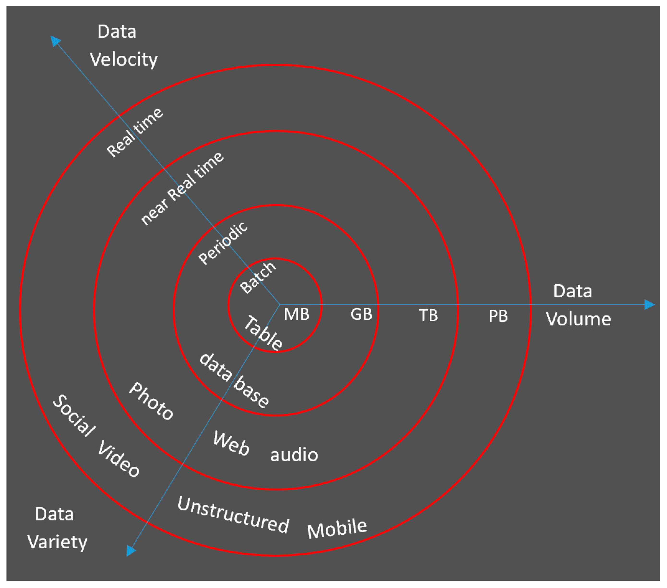
Figure 1. The 3Vs of big data (Soubra 2012).
Socsci 08 00111 g001
Figure 2. Google search trends for bomber jackets in UK and US (Boone 2016).
Socsci 08 00111 g002
Figure 3. Google Trends for bomber jackets (January 2004–February 2019) (Data Source: Google Trends, 1 February 2019).
Socsci 08 00111 g003
Figure 4. Google Trends for selected luxury fashion brands (January 2004–February 2019) (Data Source: Google Trends, 20 February 2019).
Socsci 08 00111 g004
Figure 5. Google Trends for “Dolce & Gabbana” over the past 12 months. (Data Source: Google Trends, 12 March 2019).
Socsci 08 00111 g005
Figure 6. Google Trends for smart watches (January 2004–February 2019). (Data Source: Google Trends, 20 February 2019).
Socsci 08 00111 g006
Figure 7. Google Trends for different product categories in USA and UK (January 2014–March 2019). (Data Source: Google Trends, 24 March 2019).
Socsci 08 00111 g007aSocsci 08 00111 g007b
Figure 8. Seasonal plot of “Burberry” Google Trends (January 2012–December 2018). (Data Source: Google Trends, 10 February 2019).
Socsci 08 00111 g008
Figure 9. Google Trends for “Burberry” (January 2014–February 2019). (Data Source: Google Trends, (10 February 2019).
Socsci 08 00111 g009
Figure 10. Out-of-sample forecasts for “Burberry” fashion consumer Google Trends at h = 1 month-ahead from ARIMA and NNAR models.
Socsci 08 00111 g010
Figure 11. Singular spectrum analysis (SSA) signal extractions for “Burberry” fashion consumer Google Trends.
Socsci 08 00111 g011
Figure 12. Out-of-sample forecasts for “Burberry” fashion consumer Google Trends at h = 1 month-ahead.
Socsci 08 00111 g012
Figure 13. Time series plot and scatterplot for Burberry fashion consumer Google Trends: web search vs. Google shopping (Data Source: Google Trends, 14 March 2019).
Socsci 08 00111 g013
Figure 14. Time series plots for fashion consumer Google Trends on Edited’s 2019 trending colour ways for men’s clothing (Data Source: Google Trends, 24 March 2019).
Socsci 08 00111 g014
Table 1. Out-of-sample forecasting root mean square error (RMSE) results for “Burberry” fashion consumer Google Trends.
HorizonARIMAETSTBATSNNAR
12.302.522.423.08
32.762.902.754.13
62.992.983.074.06
123.533.303.503.79
Note: Shown in bold font is the best performing univariate model at each horizon.
Table 2. Out-of-sample forecasting RRMSE results for “Burberry” fashion consumer Google Trends.
HorizonARIMAETSTBATSNNAR
10.72 *0.65 *0.68 *0.53 *
30.71 *0.67 *0.71 *0.47 *
60.73 *0.73 *0.71 *0.54 *
120.800.860.810.75
Note: * indicates the differences between forecasts are statistically significant based on the Hassani-Silva test (Hassani and Silva 2015a) at the 10% significance level.