Article

Accounting for Demography and Preferences: New Estimates of Residential Segregation with Minimum Segregation Measures

by
Jeffrey M. Timberlake
Department of Sociology, University of Cincinnati, 1018 Crosley (ML 0378), Cincinnati, OH 45221-0378, USA
Soc. Sci. 2018, 7(6), 93; https://doi.org/10.3390/socsci7060093
Submission received: 8 May 2018 / Revised: 25 May 2018 / Accepted: 30 May 2018 / Published: 6 June 2018

Abstract

:
The index of dissimilarity (D) has historically been and continues to be a widely used quantitative measure of residential segregation. Conventional interpretations of D imply that normatively desirable residential patterns occur when ethnoracial compositions of lower-order geographic units (such as neighborhoods) match those of higher-order units (such as metropolitan areas). However, it is likely that average preferences for same-group contact in neighborhoods sometimes exceed group population shares in metropolitan areas. In such situations, there is mathematical tension between the capacity for group preferences for co-ethnic neighbors to be satisfied and the degree of residential segregation. In this article, I quantify this tension by calculating , or the difference between D and the minimum segregation measure D*, which returns the lower bound on segregation for a given average in-group preference level and ethnoracial share. Positive scores on indicate that a metropolitan area is more segregated than necessary to satisfy average group preferences, while negative scores indicate that observed residential patterns do not satisfy such preferences. I use data from the 2010 decennial census and 2006–2010 American Community Survey to analyze the associations between predictors of residential segregation and .

1. Introduction

Residential patterns have captured the attention of social scientists for nearly a century (Park 1926; Burgess 1928). However, the quantitative measurement of ethnoracial segregation began in earnest during the decade immediately following World War II (Jahn et al. 1947; Cowgill and Cowgill 1951; Duncan and Duncan 1955). Following the publication of Duncan and Duncan (1955) seminal review of segregation indexes—ushering in what Massey and Denton (1988, p. 281) call the Pax Duncana—most quantitative analyses of segregation have featured, inter alia, the index of dissimilarity (D). Although several methodological weaknesses have been noted (Cortese et al. 1976; Winship 1977; White 1983), D continues to be widely employed in the literature (Iceland et al. 2013; Parisi et al. 2015).
D measures the extent to which the demographic composition of more fine-grained geographic units (such as census block groups or tracts) matches the composition of more coarse-grained units (such as cities or metropolitan areas). As calculated in Equation (1) below, it ranges from 0 to 100 and is frequently interpreted as the percentage of one group that would have to move in order to achieve a completely even distribution. As noted by Winship (1977), the problem with this interpretation is that it requires that the members of one group move into neighborhoods disproportionately occupied by another group, “assuming that no one in the other group moved out of those [neighborhoods]” (p. 1061). Moreover, the percentage of one group (or the other) that would have to move depends on the precise demographic makeup of the city or metropolitan area.
A more realistic and accurate definition of D is that of a deviation, or the difference between the empirical distribution of two groups and a counterfactual distribution in which all members of the two groups live in lower-order geographic units with the same demographic composition as the higher-order unit (yielding a D score of 0). Figure 1 in Duncan and Duncan (1955, p. 212) nicely demonstrates this interpretation of D as a deviation, showing that it is the “maximum vertical distance between the diagonal [i.e., no segregation] and the [Lorenz] curve,” or a plot of the tract cumulative proportion of nonwhites on the horizontal axis and whites on the vertical axis. Similarly, Winship (1977) refers to D as measuring “a deviation from complete desegregation” (p. 1065).
Massey and Denton (1993) offer the rule of thumb that D scores above 60 are “high,” between 30 and 60 are “moderate,” and below 30 are “low.” Although there is not an intrinsically normative connotation to these terms, most analysts imply that “high” segregation scores are undesirable and “low” scores are desirable.2 I argue that this interpretation of D is limited because it assumes that the most normatively desirable residential pattern is one in which groups are perfectly evenly distributed (i.e., the deviation between the empirical world and this particular counterfactual world is 0). It does not take into account the possibility that groups may be willing—or even prefer—to trade evenness of population distribution for same-group contact in neighborhoods. If true, then such preferences take on added importance in light of the constraining effects of the ethnoracial demography of higher-order geographic units.
To understand these constraining effects, consider the following: estimates derived from the Multi-City Study of Urban Inequality (MCSUI) indicate that black respondents report average preferences for neighborhoods that are 33 to 64% black across the four metropolitan areas surveyed in the MCSUI (see Table 1 below). Yet blacks make up between 7% and 32% of these four metropolitan areas; hence, in order for blacks to achieve a D score of 0 they would have to live in neighborhoods that are somewhat to substantially less black than their reported average preferences. Put conversely, if blacks are to live in neighborhoods that match their reported preferences, they must mathematically experience at least some level of segregation.
That level is well described by “minimum segregation measures” (Massey and Gross 1991; Fossett 2004), which indicate “the theoretical minimum level of racial residential segregation that can be achieved without violating individual preferences” (Fossett 2004, p. 2, emphasis in original). Conceptually, minimum segregation measures record the level of segregation that would exist if the households of two groups A and B were placed strategically into neighborhoods so as to maximize two desiderata: first, members of group A’s preference for same-group contact (or, alternatively, separation from members of group B) must be satisfied, and second, segregation must be kept at the minimum possible level to achieve the first goal. Hence, minimum segregation measures reveal the degree to which an aggregate-level demographic outcome such as residential segregation can be affected by preferences, especially in particular demographic contexts.
Although several minimum segregation measures exist (Fossett 2004, p. 16), in this article I focus on D*, which can be used to derive the minimum level of segregation any group would require to match their preferences for neighborhood ethnoracial composition. Massey and Gross (1991) originally employed a version of this measure to analyze the minimum amount of segregation that whites would require to keep their exposure to blacks at desired levels. Errors in their formula were subsequently identified by Krivo and Kaufman (1999) and Fossett (2004). In this article, I employ the corrected formula used by Fossett (2004) and analyze data from the 2010 decennial census to calculate D and D* scores for non-Latino whites, blacks, and Asians, and Latinos of all races. I then subtract D* from D to arrive at , or the extent to which a metropolitan area’s observed level of segregation exceeds or falls short of its associated hypothetical minimum score. I present descriptive statistics for this variable and then regress the values on measures derived from prior research on determinants of residential segregation.

2. Goals and Contributions

Before proceeding, I wish to specify the precise goals of this study and suggest some of its contributions. To begin with, I do not claim that preferences for same-group contact are the only or even primary cause of historical or contemporary residential segregation. Historically, segregation was constructed via unalloyed racism, ranging from the terrorism of in-migrating blacks by white citizens (Drake and Cayton 1945; Sugrue 1996) to the practice of redlining carried out by federal government agencies and private mortgage lenders from the mid-1930s until the late 1960s (Massey and Denton 1993). Although recent research suggests that overt discrimination in housing markets is on the wane (Ross and Turner 2005), more subtle forms may continue to target minority home seekers (Massey and Lundy 2001; Turner et al. 2013).
Contemporary residential patterns are the dynamic outcomes of thousands of household-level decisions made in the context of a large set of complex social conditions (Bruch 2014). Hence, although some component of residential decision-making may represent the exercise of preferences, those preferences are shaped by the experiences of living in a society with a long history of deep ethnoracial inequities and ongoing levels of advantage and disadvantage distributed unevenly across categories of achievement and ascription (Tilly 1998; Massey 2007). Thus, the term “preferences” should neither denote nor connote, to paraphrase Zubrinsky and Bobo (1996), “morally innocent ethnocentrism” (p. 372). Rather, research has suggested that preferences are likely a multidimensional construct, comprising elements of both homophily and out-group antipathy (Bobo and Zubrinsky 1996; Zubrinsky and Bobo 1996; Charles 2000; Timberlake 2000; Krysan 2002a, 2002b; Krysan and Farley 2002; Krysan and Bader 2007; Krysan et al. 2009).3
In this article, I address neither the determinants nor moral standing of preferences for neighborhood ethnoracial composition. I assume that these preferences (1) exist, at least in latent form, (2) represent one of several maximands in the residential decision-making process, and (3) comprise both positive in-group and negative out-group sentiment. Analytically, I seek to understand their potential implications for interpreting empirical levels of segregation. Put differently, I wish to highlight the fact that normative interpretations of D rest on one particular counterfactual—completely even population distribution—and to show that this is not the only possible counterfactual against which to evaluate levels of segregation. Put differently, the measure I introduce in this article retains the interpretation of segregation of a deviation, but a deviation from a different counterfactual than the one implied by D. In sum, I ask the following question: what new insights can be drawn from evaluating segregation as a deviation not from even population distribution, but from the level that would exist if groups’ average preferences for same-group contact were satisfied, conditional on the shares of those groups in metropolitan areas?
I stress that my estimates depend on one empirical value—group population shares—and one hypothetical (though derived from representative survey data) value—average in-group preferences. I believe that this exercise in “hypothetical demography” makes two important contributions to the literature on residential segregation. First, whereas prior studies using the index of dissimilarity either remain silent on the issue of the “desirable” level of segregation or, more commonly, imply that desirability refers to very low levels of segregation, the approach followed here allows for the notion of desirability to vary. Second, my estimates explicitly account for variation in the ethnoracial composition of metropolitan areas. Measures of this composition are frequently entered in the right-hand side of regression equations predicting levels of segregation; however, the estimates presented here incorporate this variation into the indicator itself. Overall, my findings suggest that one reason for the relative intransigence of segregation over time may be that—given the ethnoracial distributions that currently exist in most US metropolitan areas—groups face two inversely related demographic outcomes: (1) satisfaction of preferences for in-group contact and (2) residential segregation.

3. Theoretical Background

In the sections below, I provide a brief overview of empirical findings regarding patterns and determinants of ethnoracial segregation. In addition, interested readers should consult Timberlake and Ignatov (2014) and reviews of the theoretical explanations for residential inequality found in Farley and Frey (1994), Charles (2003), Logan et al. (2004), and Timberlake and Iceland (2007).
Findings from recent research show that, in 2010, African Americans continued to be the most segregated ethnoracial group in the United States. Logan and Stults (2011) report that the average weighted (by the metropolitan area minority population) black-white D score was 59 in 2010, compared to 49 for Latino-white and 41 for Asian-white. Findings from analyses of census data from 1980 to 2010 also indicate that while black segregation has declined modestly over time, segregation among Latinos and Asians has stagnated or even increased (Massey and Denton 1987; Farley and Frey 1994; Timberlake and Iceland 2007; Logan and Stults 2011). This latter trend likely results from high levels of immigration during the 1980s and 1990s (Iceland 2009). Heavy flows of new immigrants may have increased the size and density of residential enclaves, including “ethnic communities” located in the suburbs of metropolitan areas (Logan et al. 2002; Hall 2013). Such flows would cause segregation to increase in cities that are popular destinations for Latino and Asian immigrants. As a result, the Latino population experienced as much segregation in 2010 as it did in 1970, and the foreign-born population overall was more segregated in 2010 than in 1970 (Logan and Stults 2011).

3.1. Spatial Assimilation Theory

Spatial assimilation theory (Massey and Mullan 1984; Massey and Denton 1985) posits that immigrant groups experience a process towards residential integration in part via acculturation, or adopting the language and cultural practices of a society’s majority group. Indeed, numerous empirical studies confirm that English language acquisition is positively associated with spatial assimilation (Logan et al. 1996; Massey and Denton 1987; Iceland 2009). A second engine of spatial assimilation, according to spatial assimilation theory, is socioeconomic mobility. Ethnoracial groups tend to start at the bottom of the socioeconomic ladder and therefore are only able to purchase residence in low-SES neighborhoods. As these groups experience mobility, they convert increases in household SES into upward residential mobility, resulting in their occupying higher-status neighborhoods (Massey and Denton 1985). Empirical evidence from prior research indicates that SES plays a moderate role in explaining patterns of segregation for Latinos and Asians and less so for African Americans, though the spatial assimilation returns to SES have increased for blacks over time (Logan et al. 2004; Iceland 2009).
Finally, ethnoracial preferences can be incorporated into spatial assimilation theory, because preferences for (or against) other-group contact are intimately linked to the entire assimilation process, what Gordon (1964) calls “identification assimilation.” Contemporary scholarship on residential preferences follows the work of Schelling (1971), who demonstrated that micro-level residential choices can result in aggregate patterns of residential segregation. More sophisticated simulation models have followed in the footsteps of Schelling, incorporating multiple types of preferences, several ethnic groups, urban demographic composition, and intergroup inequality in socioeconomic status (Fossett and Waren 2005; Fossett 2006; Clark and Fossett 2008). These studies show that although group differences in preferences for same-group contact are not necessary to produce high levels of simulated segregation, they can be sufficient. In Fossett’s words, “the persistence of segregation in recent decades may have been overdetermined, that is, it may have been sustained by multiple sufficient causes including not only discrimination, but also social distance and preference dynamics” (Fossett 2006, p. 185).
The primary objection to the conclusions drawn from formal modeling and simulation techniques comes from research on the determinants and levels of in-group preferences. These studies show that blacks report more willingness to live in integrated neighborhood settings than whites do, and that a primary determinant of whites’ in-group preferences is negative out-group affect, not pure homophily (Bobo and Zubrinsky 1996; Zubrinsky and Bobo 1996; Timberlake 2000; Emerson et al. 2001; Krysan and Bader 2007; Krysan et al. 2009). For example, using an innovative design in which investigators showed experimentally manipulated video clips of neighborhoods to respondents, Krysan et al. (2009) found that whites were more sensitive than blacks to neighborhood racial composition and that whites who espoused negative attitudes toward blacks were especially sensitive to racial composition.
I do not dispute the evidence that ethnoracial minorities are more tolerant of integration than are whites, nor that a larger component of whites’ stated preferences is out-group antipathy than is true of blacks or other minority groups. However, neither of these stipulations vitiates the claim that ethnoracial preferences might have a large impact on the residential decision-making of both whites and minorities (see footnote 3 above). In other words, even if whites’ stated preferences for same-group contact are entirely due to out-group antipathy, and minorities’ preferences are driven entirely by in-group affinity, these factors would still serve to perpetuate high levels of segregation. Furthermore, even if minority groups are more tolerant than whites of living in mixed environments, segregation would persist if the supply of mixed neighborhoods at any given time is low. In such situations, minority preferences may not be able to be realized, and therefore potential movers must choose between neighborhoods with high concentrations of their own or another group. As Grauwin et al. (2012) argue, “large segregative patterns appear although they absolutely do not maximize the utility of most agents … one of the key element (sic) driving segregation is … the fact that even if the agents have a strict preference for mixed environments, they still prefer to belong to the majority group instead of being in (sic) minority” (p. 132).

3.2. Place Stratification

Hence, the primary tenet of spatial assimilation theory is that individuals and families make residential decisions based on exogenously-determined tastes and preferences for neighborhood characteristics and on their economic wherewithal. Proponents of the place stratification perspective acknowledge that SES and other household-level characteristics are important determinants of residential location, but in addition emphasize the role of discrimination in shaping residential patterns (Logan 1978; Logan and Molotch 1987). More specifically, negative out-group sentiments may both trigger discriminatory behavior among majority group members and become embedded in government, financial, insurance, and real estate institutions, leading to the exclusion of minority group members from certain communities. As a result, minority group members are constrained in the process of “locational attainment” or in their ability to translate their preferences and socioeconomic characteristics into desired residential outcomes. Indirect empirical support for the place stratification perspective comes from historically high levels of segregation and from inequalities in locational attainment. For example, middle-class blacks tend to live in neighborhoods with significantly lower median incomes and higher poverty rates than statistically comparable white (Logan et al. 1996; Alba et al. 2000; Reardon et al. 2015). In addition, scholars have documented discrimination in housing markets against African Americans, and to a lesser extent Latinos and Asians, through the use of audit studies (Massey and Lundy 2001; Ross and Turner 2005; Turner et al. 2013).
More direct empirical support has been limited largely due to a lack of data that clearly demonstrate effects of discrimination on lower levels of locational attainment for minorities. Researchers sympathetic to the place stratification perspective frequently conclude that, after controlling for measures suggested by the spatial assimilation model, residual ethnoracial inequality should be interpreted as the combined effects of discrimination. Yet some unknown portion of such residuals could be generated by other processes—for example, minority families’ decisions to trade residential integration with whites for propinquity to close friends and extended family members, churches or other community-based institutions, or simply more densely populated urban cores. Therefore, the findings I present should be interpreted as an assessment of the impact of variables suggested by the spatial assimilation model, not an adjudication between the spatial assimilation and place stratification perspectives.

3.3. Ecological Context

A third set of predictors of residential patterns has been grouped under the rubric “ecological context.” These are typically characteristics of metropolitan areas that are thought to constrain or abet the operation of spatial assimilation processes and to have effects on segregation in their own right. For example, cross-sectional research has found that inter-city variation in segregation was associated with the region, “functional specialization” (e.g., the concentration of manufacturing jobs or retirement-age population), size, proportion minority, population growth, and income inequality of metropolitan areas (Iceland et al. 2013). Logan et al. (2004) found that the segregation of blacks and Latinos from white was considerably lower in southern and western metro areas, though region was less important for white-Asian segregation. On average, metro areas devoted to retirement and durable goods manufacturing had more white-black segregation, and those with functional specializations in government, military, and higher education were less segregated. Finally, metropolitan areas with newer housing stock tend to be less segregated than those with older housing stock (Timberlake and Iceland 2007).

4. Data and Variables

4.1. Data

The data for this article come from two general sources. First, I calculate D scores and independent variables with data from the 2010 US Decennial Census and the 2006–2010 American Community Survey. Second, I generate plausible estimates of average in-group preferences with data from the 1992–1994 MCSUI, the 2004 Detroit Area Study (DAS), the 2004–2005 Chicago Area Study (CAS), and the 2000 General Social Survey (GSS).4 Although the methods described in this article allow for many possible preference levels, I establish baseline estimates through the use of these data.
The units of analysis are all Core-Based Statistical Areas (CBSAs)5 defined in the 2010 census. I eliminate CBSAs with fewer than 2500 members of each ethnoracial group taken in turn because segregation indexes calculated with small group populations can be unreliable (Logan et al. 2004; Iceland et al. 2013). This selection criterion yields 933 CBSAs for whites, 499 for blacks, 248 for Asians, and 586 for Latinos.

4.2. Dependent Variable

The dependent variable is the difference between the observed level of segregation experienced by non-Latino whites, blacks, and Asians, and Latinos of all races—with each group compared to all others (including members of “other races”)—and the minimum level of segregation required to satisfy each group’s hypothetical (though, again, derived from survey estimates) preferences for same-group neighbors. For the empirical measure of segregation, I compute the index of dissimilarity, at the block group level for each CBSA as
D = 0.5 ( i = 1 I | a i A b i B | ) · 100
where ai and bi are the number of members of groups A and B in block group i, and A and B are the number of members of groups A and B in the CBSA. As noted above, D ranges from 0 to 100, with higher scores indicating more difference between the empirical distribution of the population and a completely even distribution (registered by a D score of 0).
The minimum segregation measure is D*. As discussed in Fossett (2004, p. 31), D* can be calculated as
D * = ( 1 A / T B / T · ( 1 δ ) δ ) · 100   ( for   A / T > δ ;   0   otherwise ) ,
where A and B are as described above, T is the total CBSA population, and δ is the average proportion of own-group neighbors desired by group A. Equation (2) simplifies somewhat to
D * = ( 1 ( A A δ ) B δ ) · 100
and the difference between D and D*, which I abbreviate in this article as , is
D Δ = D D *
Hence, the quantity is the difference between the observed level of segregation (as measured by D) experienced by group A and the minimum level group A would experience if they were to live in neighborhoods that satisfied their average preferences for neighborhood ethnic composition (assuming indifference to the precise ethnoracial makeup of group B), accounting for their share of the CBSA population. Positive scores on indicate that a CBSA is more segregated than is necessary to satisfy the average ethnoracial preferences of group A, while negative scores indicate that observed residential patterns do not satisfy such preferences.

4.3. Estimates of In-Group Preferences

Equation (3) indicates that the magnitude of depends on both the ethnoracial composition of a city or metropolitan area (captured in the values for A and B) and the choice of the parameter δ. Ideally, I would be able to estimate δ for each ethnoracial group in each CBSA (see footnote 4). However, because those data are not available, I derive plausible estimates of δ from several sources. First, the MCSUI—administered in the early 1990s in Atlanta, Boston, Detroit, and Los Angeles—contains questions regarding the desired number of same-group “houses” in an imaginary 15-house “neighborhood.” Asian, black, and Latino (but not non-Latino white) respondents were presented show cards with 15, 10, 7, 2, and 0 same-group houses colored in on the cards and asked to rank them in terms of preference from most to least desirable. I took a weighted average of the percentage of same-group neighbors (with the number of respondents choosing each “neighborhood” as the weights) for the first- and second-most desirable neighborhoods and then averaged those percentages, giving two-thirds weight to the first preference and one-third weight to the second preference. Similar questions were asked of blacks on the 2004 DAS, about a decade after the fielding of the MCSUI.6
A second measure of preferences comes from questions on the Boston and Los Angeles MCSUI surveys, as well as the DAS, CAS, and GSS. Here respondents were given a blank 15-house show card and asked to fill in the houses with one of several (depending on the survey) ethnoracial groups. For each survey and city, I calculated the average percentage of own-group members desired by whites, Asians, blacks, and Latinos. Results of these calculations are shown in Table 1 in the rows labeled “ideal neighborhood.” In order to account for variability in the cities and in the two methods, I took a weighted (by the survey sample sizes) average of each group’s preferences, shown in Table 1 in the bolded row titled “Overall average.” Note that average preferences all exceed 50%, with Asians expressing preferences for higher levels of in-group contact (driven largely by the Los Angeles portion of the MCSUI).
Using the data from Table 1 (where δ is the value for each group in the bolded “overall average” row), I calculate D* scores for blacks ranging from 58.7 in Atlanta to 93.7 in Boston and Los Angeles. Because Atlanta, Chicago, and Detroit have higher percentages of blacks than Boston and Los Angeles, less segregation (again, measured in terms of D) is necessary to satisfy blacks’ specified preferences for same-group contact. D* scores for Asians and especially Latinos are lower in Los Angeles than in the other cities, owing to the relatively large Asian and Latino populations in LA. Finally, D* scores for whites are estimated to be zero in Boston, Chicago, and Detroit, due to the relatively high percentage of whites in these three metropolitan areas (75%, 55%, and 68% in 2010, respectively).

4.4. Independent Variables

I predict with a variety of independent variables shown in past literature to be associated with segregation scores in cross-sectional analyses. These include several measures of spatial assimilation and additional measures of ecological context, which capture historical and structural forces that may affect segregation levels.
I capture the two central propositions of spatial assimilation theory—that acculturation and socioeconomic mobility lead to minority spatial assimilation—by estimating effects of four metropolitan area-level variables on 2010 levels of . I operationalize acculturation as the CBSA-level percentage of each group that speaks English very well. I measure socioeconomic status as the percentage of each group who have a college degree or more, the percentage of each group owning their own homes, and the ratio of each group’s median household income relative to that of the other three groups combined.
Following the examples of much prior research, I assess the impact of ecological context on levels of and changes in residential inequality. First, I control for several population characteristics, including the natural log of population size and the percentage of each CBSA’s population that lives in the suburbs. I control for the “functional specialization” of CBSAs (Farley and Frey 1994) by controlling for the percentage of employed workers age 16 and over in the manufacturing and government sectors, and the percentage of the population age 65 and over, frequently used to operationalize retirement communities. I include the percent foreign born of each group to account for the tendency of immigrants to settle in segregated enclaves in particular CBSAs. Additionally, I include several measures of housing supply because processes of integration on the availability of housing both in neighborhoods undergoing transition and in neighborhoods into which departing residents can move. I measure both the CBSA-level percentage of vacant housing and the median year the CBSA’s housing was built, to capture the degree to which residential patterns are likely to be older and therefore more entrenched. Finally, I control for region by including dummy variables for the census region of the CBSA. Means and standard deviations for all variables used in the analysis are shown in Table 2 below.

5. Descriptive Findings

My analysis proceeds in two steps. First, Figure 1 provides descriptive analyses of the distributions of by ethnoracial group and three hypothetical preference levels (δ = 0.25, 0.50, and 0.75), while Figure 2 presents average scores across a range of values of δ in 5-point increments. Second, I analyze the results from ordinary least squares regression models showing the associations between the independent variables and , holding the value of δ at 0.50.7

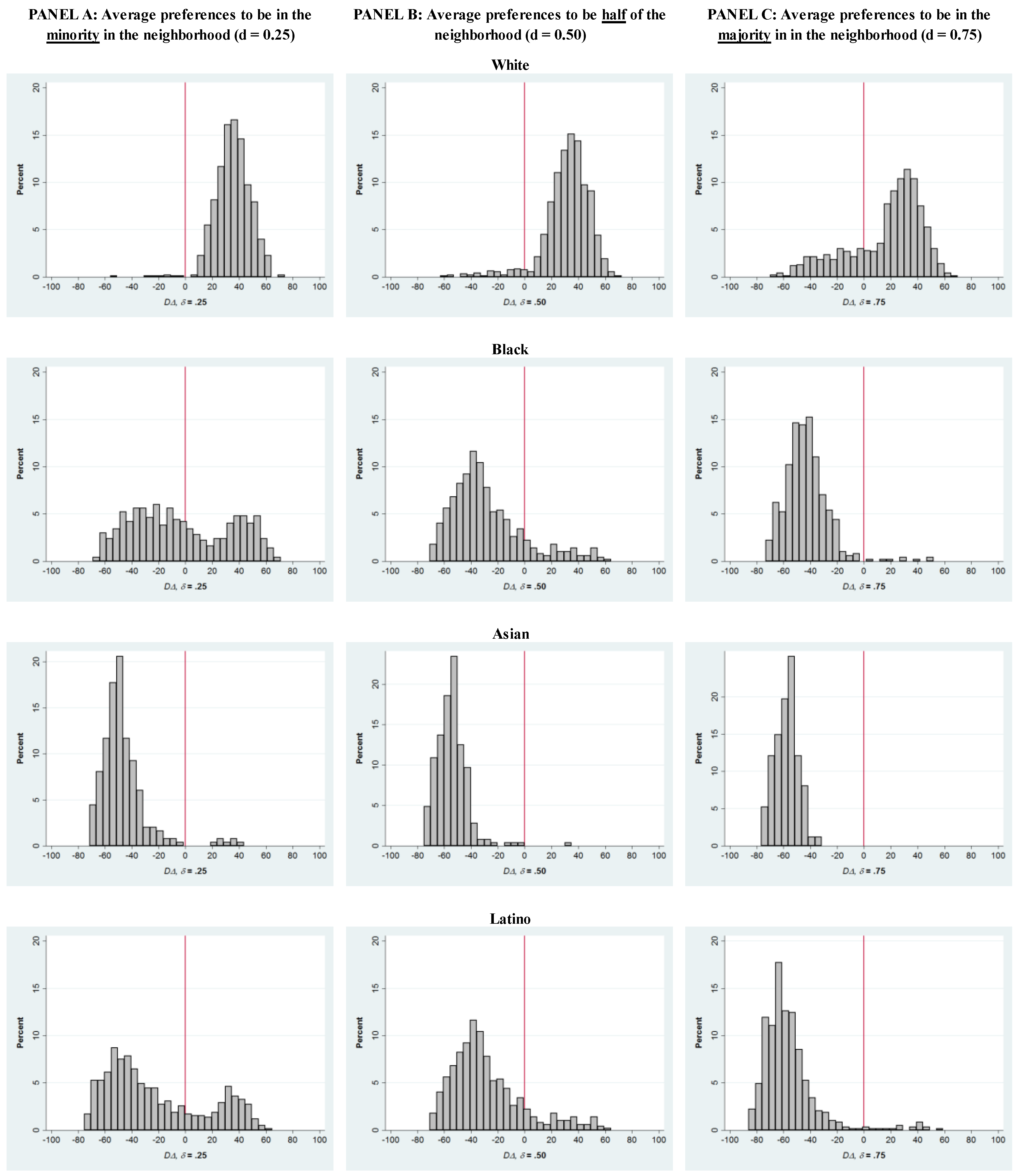
5.1. Distributions of DΔ

Figure 1 below shows histograms of for the four ethnoracial groups under consideration. The class widths are five points and the vertical red line marks the 0 point on the horizontal axis. Recall that positive scores indicate that a CBSA is more segregated than necessary to achieve the average preferences of a group for own-group neighborhood composition, while negative scores indicate that the observed residential patterns do not enable groups to achieve (assumed) average preferences for in-group contact. Histogram A for whites shows that virtually all CBSAs are more segregated than necessary to enable whites to live in neighborhoods that are at least 25% white. This is not surprising, given that most CBSAs feature white shares well in excess of 25%. Exceptions are CBSAs with relatively small white populations, such as Brownsville-Harlingen, TX (11.4% white), El Paso, TX (13.5%), and El Centro, CA (14.7%). Using El Paso as an example, in 2010, the observed white-other index of dissimilarity score was 42.9, whereas the minimum segregation score was 54.6. Thus, in order for all whites in the El Paso metropolitan area to live in neighborhoods that were at least 25% white, segregation would have to correspond to a D score of 54.6. Hence, El Paso is 11.7 index of dissimilarity points “too low” to grant whites residential preferences corresponding to δ = 0.25 (42.9 − 54.6 = −11.7).
Of course, these CBSAs are in the vast minority; far more common is for segregation scores to be higher than necessary for whites to achieve hypothetical average preferences for white neighborhoods. In some cases, these are CBSAs with white populations large enough that the percentage white exceeds the δ value of 0.75 (see histogram A3), such as the Buffalo-Cheektowaga-Niagara Falls, NY CBSA, at 80.1% white. Because this percentage exceeds 75%, it would be possible for the white-nonwhite D score to be 0 and still satisfy white preferences for 75% white neighborhoods. In fact, the observed D score in Buffalo in 2010 was 60.3, yielding a value of 60.3. Other examples of CBSAs with positive scores are ones with smaller white populations that would require some level of segregation to enable neighborhoods to be 75% white, but where the observed D scores far exceed that level. For example, with a non-Latino white population of 72.3%, the Cleveland-Elyria, OH CBSA would require a D score of just 15.4 to ensure whites’ preferences for same-group contact at δ = 0.75. However, its white-nonwhite D score in 2010 was 62.8, indicating that Cleveland-Elyria was 47.4 points “too segregated” for these hypothetical average preferences (62.8 − 15.4 = 47.4).
When δ is allowed to reach the very high level of 0.90, the distribution of CBSAs for whites becomes more uniform, with a mean of −10.7 and a median of −14.8 (data not shown here). This indicates that if whites held extreme preferences for in-group contact (or lack of out-group contact), nearly half of U.S. metropolitan areas would still be more segregated than necessary to achieve these preferences. CBSAs with scores above 0 for δ = 0.90 are those with very high non-Latino white population shares, such as Pittsburgh, PA (87.5%) and Cincinnati, OH (82.2%). Areas with white percentages that high need very little segregation to ensure 90% white neighborhoods, yet Pittsburgh’s white-other D score in 2010 was 52.9 and Cincinnati’s was 55.0. As I discuss in the concluding section, this could be seen as good news for advocates of declining segregation, in that even if whites’ average preference for white neighbors were as high as 90%, and even if these preferences were driven entirely by out-group antipathy, Pittsburgh and Cincinnati would still not need to be as segregated as they are. Of course, if white preferences were lower than 90%, then these CBSAs could support still lower levels of segregation.
For African Americans, at relatively low levels of preference for in-group contact (δ = 0.25) many CBSAs (210 of 499) are, not surprisingly, more segregated than necessary (see Figure 1, histogram B1). However, nearly three-fifths (289) of the CBSAs in this sample featured scores less than 0, indicating that blacks’ hypothetical preferences for same-group neighborhood contact would not be met, even at relatively low average preference levels. This is likely a surprising finding for most readers, yet it highlights the crucial importance of ethnoracial demography. Of the 210 CBSAs with scores above 0 for δ = 0.25, the average percent black was 29.8% in 2010, and included some of the largest and most well-known metropolitan areas in the United States, including Baltimore, Chicago, Cleveland, Detroit, Houston, New York, Philadelphia, and Washington, DC. However, the average percent black in CBSAs with negative scores was just 6.7%. In these CBSAs, it would take high levels of segregation to allow all blacks to live in neighborhoods that are as little as 25% black.
Hence, although a very large fraction of the black population lives in cities with more segregation than necessary to achieve these low levels of same-group contact, the majority of CBSAs would not satisfy blacks’ preferences for same-group neighborhoods, even if these preference levels were as low as 25%. This does not mean that blacks want or should want more segregation in those CBSAs; rather, what my analyses indicate is that desegregation and preferences for in-group contact are, in many real demographic contexts, at odds with one another.
The foregoing discussion suggests that if blacks’ preferences for same-group contact were higher than 25%, the percentage of CBSAs that do not meet blacks’ hypothetical preferences would increase. And in fact, that is what I observe in histogram B. At δ = 0.50, a figure close to the weighted average of the preferences scores in Table 1, just 66 of the 499 CBSAs in the black sample featured scores greater than 0, indicating more segregation than necessary to achieve an average preference level of 50%. Sixty-five of these were in the South, including large CBSAs such as Atlanta, Baltimore, Memphis, and New Orleans, and smaller CBSAs such as Albany and Macon, GA and Pine Bluff, AR. In the non-South, the only CBSA more segregated than necessary to achieve blacks’ hypothetical preferences for 50% black neighborhoods was Detroit. Finally, histogram C shows that if blacks’ average preferences were as high as 75% (a figure exceeding the upper bound of any of the preference data shown in Table 1), just eight CBSAs—all in Mississippi and Alabama—would be more segregated than necessary to enable these preferences.
For Asians, the distributions of vary little with respect to values of δ. Virtually all CBSAs would not allow Asians to live in neighborhoods that are even 25% Asian, with the exceptions of four CBSAs in Hawai’i (Hilo, Honolulu, Kahului-Wailuku-Lahaina, and Kapaa) and two in the San Francisco Bay Area (San Francisco-Oakland-Hayward and San Jose-Sunnyvale-Santa Clara). This is entirely due to the fact that most CBSAs have very small Asian populations.8 Hence, in the current demographic context, it would take a great deal of segregation to enable Asians to satisfy desires for same race contact even as high as 25%, to say nothing of 50% or 75%, which is close to the preference level expressed by Asians surveyed in the Los Angeles MCSUI survey (see Table 1). When δ = 0.50, the lone CBSA more segregated than necessary to achieve Asians’ hypothetical preferences is Honolulu, which had an Asian (including native Hawai’ian and other Pacific Islander) population of 52.5% in 2010 and an Asian-other D score of 31.1. Because no segregation would be necessary to ensure that Asians could live in neighborhoods that are 50% Asian, the resulting score is 31.1 − 0 = 31.1.
Finally, the distributions of for Latinos resemble those for blacks. At low levels of same-group preference (δ = 0.25) a sizeable minority (158) of the 586 CBSAs with at least 2500 Latinos are more segregated than necessary to enable all Latinos to live in neighborhoods with at least 25% Latino residents (see histogram D1). When δ shifts to 0.50 (histogram B), only 64 CBSAs remain more segregated than necessary to achieve 50% Latino neighborhoods. Not surprisingly, these are CBSAs with relatively large Latino populations, primarily in southern and western states such as Arizona, California, Florida, New Mexico, and Texas. For example, the Santa Fe, NM CBSA had a Latino population of 50.1% in 2010, meaning that no segregation would be required to ensure the 50% preference threshold. However, the Latino-other D score in Santa Fe in 2010 was 42.8, yielding a value of 42.8. At δ = 0.75, just 18 CBSAs remain more segregated than necessary to achieve neighborhood compositions of at least 75% Latinos. These CBSAs are all in Arizona (1) California (1), New Mexico (3), and Texas (13), with an average Latino percentage in 2010 of 80.8%.

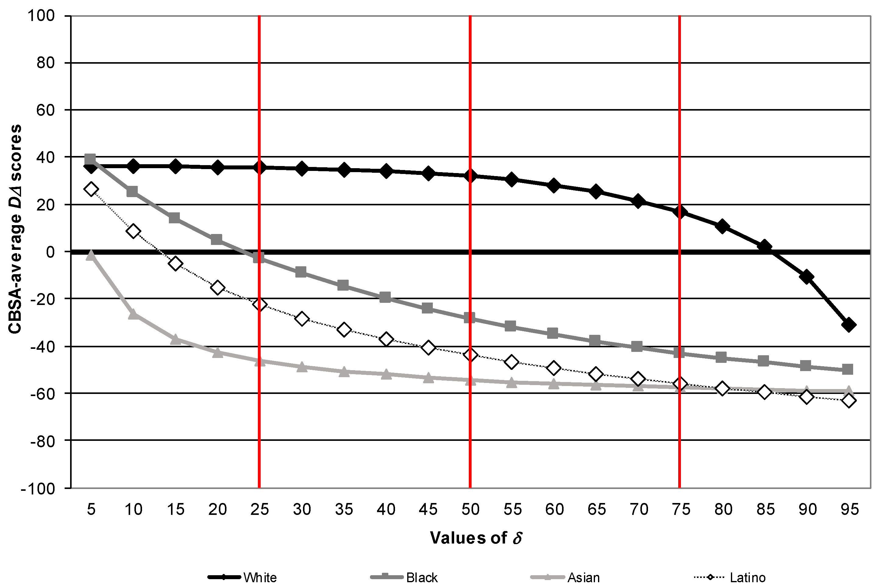
5.2. Average DΔ Scores

Figure 2 below shows CBSA-level average are all scores across the full range of plausible δ values. This analysis conceals the variation depicted in Figure 1 but allows us to explore how are all changes with respect to δ. I have added red vertical lines to match the values of δ shown in Figure 1, and bolded the zero point on the vertical axis to indicate the value of δ for which the observed level of segregation is, on average, at its minimum possible level to satisfy the assumed preferences of the four ethnoracial groups. Note that for whites, that level is achieved at very high preference levels, around 0.85. This indicates that if whites’ preferences levels were in the neighborhood of those reported on several national- and city-level surveys, whites on average live in CBSAs that are far more segregated than necessary to achieve these preferences.
For the three minority groups, Figure 2 shows the reverse pattern from that of whites, though there are stark differences between blacks and the other two groups. For Asians, even at the lowest levels of δ (0.05) presented in this analysis, average levels of Asian segregation do not enable them to achieve these preferences, at least with CBSAs as the unit of analysis. For Latinos, very low levels of δ correspond to more segregation than is necessary to achieve average preferences, but as δ exceeds about 0.12, the curves drop below the zero point. For blacks, the point at which segregation becomes does not enable hypothetical average preferences to be satisfied occurs at a δ value of about 0.20.

6. Regression Findings

The findings in Figure 1 and Figure 2 suggest that, on average, whites live in CBSAs with far more segregation than is necessary to satisfy their average neighborhood preferences, except at very high levels of preference for same-group contact (e.g., δ = 0.90). By contrast, except at very low levels of same-group preferences, minorities live in CBSAs that do not satisfy hypothetical average preferences for same-group residential contact. However, as shown in Figure 1, there is substantial variability in the scores, which issues from variation in actual segregation (measured by D) and the ethnoracial demography of each CBSA (measured by the A and B terms in Equation (3)). I next turn to an analysis of the correlates of that variability via the regression results reported in Table 3. I report coefficient and standard error estimates9 from ordinary least squares regressions of the scores (with δ = 0.50) for each group on the independent variables described above. The coefficients, then, represent the relationship between the predictors and segregation, where instead of segregation being measured as a deviation from complete desegregation (as with D), it is measured as a deviation from the minimum segregation score.
The independent variables are measured in deviation units, calculated by subtracting each CBSA’s score from the ethnoracial group mean, calculated for the CBSAs with at least 2500 members of each group. This yields constant terms that are simply the average for each group (see Table 2). Positive coefficients indicate relationships in the direction of more segregation than necessary to achieve in-group preferences and negative coefficients indicate relationships tending toward hypothetical in-group preferences not being met. As depicted in Figure 1 and Figure 2, the constant terms in the columns indicate that CBSAs that are average on all characteristics in the model are about 32 points more segregated than necessary for whites to live in neighborhoods with at least 50% white residents. By contrast, the average CBSA does not allow the three minority groups to live in neighborhoods with that degree of ethnoracial composition ( E [ D Δ | x ¯ ,   δ = 0.50 ] = −28.4 for blacks, −54.3 for Asians, and −43.8 for Latinos).
With respect to the spatial assimilation variables, I find that the percentage of whites, blacks, and Asians in a CBSA who speak English very well is associated with lower levels of segregation, while for Latinos, this coefficient is positive, indicating that where Latino English proficiency is greater, CBSAs tend to be modestly more segregated than hypothetical preferences would require.10 The size of the college-educated population is associated with more segregation for whites and Asians and less segregation for Latinos and blacks, though the latter coefficient is small relative to its standard error. The percentage of homeowners in CBSAs is associated with more segregation relative to preferences for whites, blacks, and Latinos, and relative income ratios are in the direction of too much segregation for whites and preferences not being met for blacks. More specifically, a CBSA that is average on all characteristics in the model for blacks is predicted to have a score of −28.4 (the value of the constant). For CBSAs otherwise average on all variables, one with a one-standard deviation higher black-other income ratio (about 0.80—see Table 2) would have a predicted value of about −38.4. This finding may indicate that blacks do not convert increases in relative income into residential propinquity with other groups to the degree suggested by the spatial assimilation model.
The other ecological context variables in the model evince a mix of relationships, with few systematic patterns of note. One exception is the uniformly negative association of age of housing stock and the dependent variable. This confirms past findings that metro areas with newer housing tend to have lower levels of segregation, likely because residential patterns are less firmly entrenched. I also observed large regional gaps. For whites, western CBSAs (the omitted category) are less segregated than necessary to achieve white preferences than the other regions. As suggested by the discussion of Figure 1 above, southern CBSAs on average are far more segregated than necessary to achieve blacks’ preferences, as are northeastern CBSAs for Latinos. Relative to the West, the Midwest region is associated with lower segregation for Latinos or tending toward the direction of preferences for Latino neighbors’ not being met. Again, this highlights the importance of ethnoracial demography—whereas Latinos are highly concentrated in western CBSAs and therefore require little or no segregation to meet preferences for 50% Latino neighborhoods, this is not true of CBSAs in the Midwest.

7. Conclusions

I began this article by arguing that conventional interpretations of the index of dissimilarity assume that the most normatively desirable residential pattern corresponds to neighborhood ethnoracial mixes that perfectly match the overall demography of a city or metropolitan area. I noted that this logic does not take into account either group preferences for neighborhood ethnic mix or the capacity for the ethnic demography of metropolitan areas to support such preferences, absent some degree of residential segregation. I then introduced a simple procedure for assessing the extent to which higher-order geographic units are more or less segregated than would be necessary to achieve groups’ hypothetical average preferences for same-group neighbors. This method entailed taking the difference between the observed index of dissimilarity score and D*, or the minimum segregation measure corresponding to the lower bound on segregation possible when average in-group preferences are not violated.
Descriptive analysis showed stark differences between non-Latino whites and the three large minority groups under consideration. First, at moderate to high levels of in-group preference (δ = 0.50 or 0.75), virtually all CBSAs were more segregated than necessary for whites to achieve their preferences. Only when assumed preference levels approach their theoretically plausible maximum (δ = 0.90) does the segregation level for a substantial fraction of CBSAs not support such preferences. This finding indicates that there is a high likelihood that whites would tolerate increased residential integration—assuming that their average preferences do not exceed 75% white—although I note that research has shown greater willingness for whites to live with Latinos and Asians than with African Americans (Zubrinsky and Bobo 1996).
For Asians the story is just the opposite. With the sole exception of Honolulu, each of the 248 CBSAs analyzed for Asians do not feature residential patterns that would support Asians’ achieving the observed average preference levels from MCSUI survey data. Given the relatively low percentage of Asian residents in most US metropolitan areas, it would take extraordinarily low levels of in-group preference among Asians for their level of segregation to support those preferences. Put differently, from the limited point of view of maximizing preferences for in-group neighborhood contact, Asians’ preferences for same-group neighbors, by and large, are not being and likely cannot be met in most CBSAs.
For blacks and Latinos, my descriptive analyses showed striking similarities. At relatively low levels of average in-group preference, a large majority of CBSAs do not enable these preferences. The exceptions are notable because they tend to be CBSAs that garner much scholarly and public attention due to their size or heavy representation of minorities. Hence, while it is true that a large fraction of blacks and Latinos live in CBSAs that are more segregated than necessary for their same-group residential preferences to be achieved, it is also true that (1) these gaps are not nearly as large as indicated by exclusive use of the index of dissimilarity and (2) a majority of CBSAs feature residential patterns that would not enable black and Latino populations to meet average preference levels of around 25 to 50% same-group neighbors.
Regression analyses lend additional support for these conclusions, as I found large positive gaps for blacks between midwestern and southern CBSAs and the omitted category, western CBSAs. This indicates that CBSAs in regions with historically large black populations tend to be more segregated than necessary to achieve blacks’ preferences for 50% black neighborhoods. Similarly, I found a negative gap for Latinos between midwestern CBSAs—traditionally not popular destinations for Latin American immigrants (except for Chicago)—and western CBSAs, which contain some of the highest representations of Latinos in the United States. Thus, segregation tends to be highest in CBSAs with the largest minority populations. Traditional accounts of this empirical regularity point to the threat felt by native-born whites at the rapid encroachment of large fractions of minority residents and the resulting exclusionary actions taken by whites to keep their neighborhoods ethnically homogeneous (Bobo and Hutchings 1996; Sugrue 1996). On the other hand, in CBSAs with smaller minority populations, it is at least conceivable that part of the reason for enduring segregation is the necessity for minorities to experience a sometimes substantial degree of segregation in order for same-group preferences to be at least partially satisfied.
Related to this last point, my findings suggest that there may be room for both optimism and pessimism in the data, at least to the extent that residential desegregation is a shared goal of American citizens. On the optimistic side of the ledger, I have shown that unless whites have extremely high levels of preference for in-group members, in most CBSAs there is substantial room for whites to allow greater entry of nonwhites into their neighborhoods, at least on average, even if white preferences are driven entirely by out-group antipathy. A more pessimistic interpretation of the data would point to the large number of CBSAs that do or would not enable blacks, Latinos, or Asians to achieve even relatively modest average in-group preference levels. This finding suggests that, in many CBSAs, it may be difficult to increase residential integration much further than has already occurred, or at least that further integration will come at the expense of minorities’ desires to live in neighborhoods with substantial concentrations of co-ethnics. This reasoning would suggest that future declines in residential segregation will occur in larger metro areas, where the residential preferences of blacks and Latinos are not being met due to excessive segregation. Indeed, in an analysis of change in segregation from 1970 to 2000, Timberlake and Iceland (2007) found this precise relationship—metropolitan areas with larger populations experienced steeper declines in segregation over time. This is a welcome trend for those interested in fostering residential desegregation, for such declines, though in a minority of metro areas, affect large fractions of the black and Latino populations.
In conclusion, I wish to restate what I think the findings from this research do and do not demonstrate. I have not demonstrated that segregation is driven primarily by group differences in preferences for in-group contact, nor that continued discrimination in housing markets does not continue to play an important role. Furthermore, nothing in the foregoing analyses should warrant the conclusion that ethnoracial minorities do or should want more residential segregation. I have shown that, given a set of fairly weak assumptions about average in-group preferences, residential segregation and preference satisfaction are inversely related desiderata in most demographic contexts. Accordingly, one key to continued reductions in residential segregation is increased tolerance among whites for residential contact with minority groups. This would likely trigger further declines in discrimination against ethnoracial minorities and enable minorities to achieve higher levels of co-ethnic contact with no resulting increases in residential segregation.

Acknowledgments

I thank Michael Bader for assistance with data analysis and additional comments and Mark Fossett, Matt Hall, and Maria Krysan for helpful comments on earlier drafts of this article. Any errors or opinions are solely those of the author.

Conflicts of Interest

The author declares no conflict of interest.

References

  1. Alba, Richard D., John R. Logan, and Brian J. Stults. 2000. How Segregated are Middle-Class African Americans? Social Problems 47: 543–58. [Google Scholar] [CrossRef]
  2. Bobo, Lawrence, and Vincent L. Hutchings. 1996. Perceptions of Racial Group Competition: Extending Blumer’s Theory of Group Position to a Multiracial Social Context. American Sociological Review 61: 951–72. [Google Scholar] [CrossRef]
  3. Bobo, Lawrence, and Camille L. Zubrinsky. 1996. Attitudes on Residential Integration: Perceived Status Differences, Mere In-group Preference, or Racial Prejudice? Social Forces 74: 883–909. [Google Scholar] [CrossRef]
  4. Bruch, Elizabeth. 2014. How Population Structure Shapes Neighborhood Segregation. American Journal of Sociology 119: 1221–78. [Google Scholar] [CrossRef] [PubMed]
  5. Burgess, Ernest W. 1928. Residential Segregation in American Cities. Annals of the American Academy of Political and Social Science 140: 105–15. [Google Scholar] [CrossRef]
  6. Charles, Camille Zubrinsky. 2000. Neighborhood Racial-Composition Preferences: Evidence from a Multiethnic Metropolis. Social Problems 47: 379–407. [Google Scholar] [CrossRef]
  7. Charles, Camille Zubrinsky. 2003. The Dynamics of Racial Residential Segregation. Annual Review of Sociology 29: 167–207. [Google Scholar] [CrossRef]
  8. Chetty, Raj, Nathaniel Hendren, and Lawrence F. Katz. 2015. The Effects of Exposure to Better Neighborhoods on Children: New Evidence from the Moving to Opportunity Experiment. NBER Working Paper. Cambridge: Harvard University and NBER. [Google Scholar]
  9. Clark, William A. V., and Mark Fossett. 2008. Understanding the Social Context of the Schelling Segregation Model. Proceedings of the National Academy of Sciences of the United States of America 105: 4109–14. [Google Scholar] [CrossRef] [PubMed]
  10. Cortese, Charles F., R. Frank Falk, and Jack K. Cohen. 1976. Further Considerations on the Methodological Analysis of Segregation Indices. American Sociological Review 41: 630–37. [Google Scholar] [CrossRef]
  11. Cowgill, Donald O., and Mary S. Cowgill. 1951. An Index of Segregation Based on Block Statistics. American Sociological Review 16: 825–31. [Google Scholar] [CrossRef]
  12. Drake, St. Clair, and Horace R. Cayton. 1945. Black Metropolis: A Study of Negro Life in a Northern City. Chicago: University of Chicago Press. [Google Scholar]
  13. Duncan, Otis D., and Beverly Duncan. 1955. A Methodological Analysis of Segregation Indexes. American Sociological Review 20: 210–17. [Google Scholar] [CrossRef]
  14. Emerson, Michael O., Karen J. Chai, and George Yancey. 2001. Does Race Matter in Residential Segregation? Exploring the Preferences of White Americans. American Sociological Review 66: 922–35. [Google Scholar] [CrossRef]
  15. Farley, Reynolds, and William H. Frey. 1994. Changes in the Segregation of Whites from Blacks during the 1980s: Small Steps toward a More Integrated Society. American Sociological Review 59: 23–45. [Google Scholar] [CrossRef]
  16. Fossett, Mark A. 2004. Racial Preferences and Racial Residential Segregation: Findings from Analyses Using Minimum Segregation Models. Paper presented at the Annual Meeting of the Population Association of America, Boston, MA, USA, May 1–3. [Google Scholar]
  17. Fossett, Mark A. 2006. Ethnic Preferences, Social Distance Dynamics, and Residential Segregation: Theoretical Explorations Using Simulation Analysis. Journal of Mathematical Sociology 30: 185–274. [Google Scholar] [CrossRef]
  18. Fossett, Mark, and Warren Waren. 2005. Overlooked Implications of Ethnic Preferences for Residential Segregation in Agent-based Models. Urban Studies 42: 1893–917. [Google Scholar] [CrossRef]
  19. Gordon, Milton M. 1964. Assimilation in American Life: The Role of Race, Religion and National Origins. New York: Oxford University Press. [Google Scholar]
  20. Grauwin, Sébastian, Florence Goffette-Nagot, and Pablo Jensen. 2012. Dynamic Models of Residential Segregation: An Analytical Solution. Journal of Public Economics 96: 124–41. [Google Scholar] [CrossRef] [Green Version]
  21. Hall, Matthew. 2013. Residential Integration on the New Frontier: Immigrant Segregation in Established and New Destinations. Demography 50: 1873–96. [Google Scholar] [CrossRef] [PubMed]
  22. Iceland, John. 2009. Where We Live Now: Immigration and Race in the United States. Berkeley: University of California Press. [Google Scholar]
  23. Iceland, John, Gregory Sharp, and Jeffrey M. Timberlake. 2013. Sun Belt Rising: Regional Population Change and the Decline in Black Residential Segregation, 1970–2009. Demography 50: 97–123. [Google Scholar] [CrossRef] [PubMed]
  24. Jahn, Julius A., Calvin F. Schmid, and Clarence Schrag. 1947. The Measurement of Ecological Segregation. American Sociological Review 12: 293–303. [Google Scholar] [CrossRef]
  25. Jargowsky, Paul. 1997. Poverty and Place: Ghettos, Barrios, and the American City. New York: Russell Sage. [Google Scholar]
  26. Krivo, Lauren J., and Robert L. Kaufman. 1999. How Low Can It Go? Declining Black-White Segregation in a Multiethnic Context. Demography 36: 93–109. [Google Scholar] [CrossRef] [PubMed]
  27. Krysan, Maria. 2002a. Community Undesirability in Black and White: Examining Racial Residential Preferences through Community Perceptions. Social Problems 49: 521–43. [Google Scholar] [CrossRef]
  28. Krysan, Maria. 2002b. Whites Who Say They’d Flee: Who Are They, and Why Would They Leave? Demography 39: 675–96. [Google Scholar] [CrossRef]
  29. Krysan, Maria, and Michael D. M. Bader. 2007. Perceiving the Metropolis: Seeing the City through a Prism of Race. Social Forces 86: 699–733. [Google Scholar] [CrossRef]
  30. Krysan, Maria, and Reynolds Farley. 2002. The Residential Preferences of Blacks: Do they Explain Persistent Segregation? Social Forces 80: 937–80. [Google Scholar] [CrossRef]
  31. Krysan, Maria, Mick P. Couper, Reynolds Farley, and Tyrone A. Forman. 2009. Does Race Matter in Neighborhood Preferences? Results from a Video Experiment. American Journal of Sociology 115: 527–59. [Google Scholar] [CrossRef]
  32. Logan, John R. 1978. Growth, Politics, and the Stratification of Places. American Journal of Sociology 84: 404–16. [Google Scholar] [CrossRef]
  33. Logan, John R., and Harvey L. Molotch. 1987. Urban Fortunes: The Political Economy of Place. Berkeley: University of California Press. [Google Scholar]
  34. Logan, John, and Brian J. Stults. 2011. The Persistence of Segregation in the Metropolis: New Findings from the 2010 Census. Census Brief Prepared for Project US2010. Available online: http://www.s4.brown.edu/us2010 (accessed on 1 May 2015).
  35. Logan, John R., Richard D. Alba, and Shu-Yin Leung. 1996. Minority Access to White Suburbs: A Multiregional Comparison. Social Forces 74: 851–81. [Google Scholar] [CrossRef]
  36. Logan, John R., Richard D. Alba, and Wenquan Zhang. 2002. Immigrant Enclaves and Ethnic Communities in New York and Los Angeles. American Sociological Review 67: 299–322. [Google Scholar] [CrossRef]
  37. Logan, John R., Brian J. Stults, and Reynolds Farley. 2004. Segregation of Minorities in the Metropolis: Two Decades of Change. Demography 41: 1–22. [Google Scholar] [CrossRef] [PubMed]
  38. Massey, Douglas S. 1990. American Apartheid: Segregation and the Making of the Underclass. American Journal of Sociology 96: 329–57. [Google Scholar] [CrossRef]
  39. Massey, Douglas S. 2007. Categorically Unequal: The American Stratification System. New York: Russell Sage Foundation. [Google Scholar]
  40. Massey, Douglas S., and Nancy A. Denton. 1985. Spatial Assimilation as a Socioeconomic Outcome. American Sociological Review 50: 94–106. [Google Scholar] [CrossRef]
  41. Massey, Douglas S., and Nancy A. Denton. 1987. Trends in the Residential Segregation of Blacks, Hispanics, and Asians: 1970–1980. American Sociological Review 52: 802–25. [Google Scholar] [CrossRef]
  42. Massey, Douglas S., and Nancy A. Denton. 1988. The Dimensions of Residential Segregation. Social Forces 67: 281–315. [Google Scholar] [CrossRef] [Green Version]
  43. Massey, Douglas S., and Nancy A. Denton. 1993. American Apartheid: Segregation and the Making of the Underclass. Cambridge: Harvard University Press. [Google Scholar]
  44. Massey, Douglas S., and Mitchell L. Eggers. 1990. The Ecology of Inequality: Minorities and the Concentration of Poverty 1970–1980. American Journal of Sociology 95: 1153–88. [Google Scholar] [CrossRef]
  45. Massey, Douglas S., and Mary J. Fischer. 2000. How Segregation Concentrates Poverty. Ethnic and Ethnic Studies 23: 670–91. [Google Scholar] [CrossRef]
  46. Massey, Douglas S., and Andrew B. Gross. 1991. Explaining Trends in Residential Segregation, 1970–1980. Urban Affairs Quarterly 27: 13–35. [Google Scholar] [CrossRef]
  47. Massey, Douglas S., and Garvey Lundy. 2001. Use of Black English and Racial Discrimination in Urban Housing Markets: New Methods and Findings. Urban Affairs Review 36: 452–69. [Google Scholar] [CrossRef]
  48. Massey, Douglas S., and Brendan P. Mullan. 1984. Processes of Latino and Black Spatial Assimilation. American Journal of Sociology 89: 836–73. [Google Scholar] [CrossRef]
  49. Massey, Douglas S., Andrew B. Gross, and Kumiko Shibuya. 1994. Migration, Segregation, and the Geographic Concentration of Poverty. American Sociological Review 59: 425–45. [Google Scholar] [CrossRef]
  50. Parisi, Domenico, Daniel T. Lichter, and Michael C. Taquino. 2015. The Buffering Hypothesis: Growing Diversity and Declining Black-White Segregation in America’s Cities, Suburbs, and Small Towns? Sociological Science 2: 125–57. [Google Scholar] [CrossRef]
  51. Park, Robert E. 1926. The Urban Community as a Spatial Pattern and Moral Order. In Urban Community. Edited by Ernest Watson Burgess. Chicago: University of Chicago Press, pp. 3–18. [Google Scholar]
  52. Quillian, Lincoln. 2012. Segregation and Poverty Concentration: The Role of Three Segregations. American Sociological Review 77: 354–79. [Google Scholar] [CrossRef] [PubMed]
  53. Reardon, Sean F., Lindsay Fox, and Joseph Townsend. 2015. Neighborhood Income Composition by Household Race and Income, 1990–2009. Annals of the American Academy of Political and Social Science 660: 78–97. [Google Scholar] [CrossRef]
  54. Ross, Stephen L., and Margery Austin Turner. 2005. Housing Discrimination in Metropolitan America: Explaining Changes between 1989 and 2000. Social Problems 52: 152–80. [Google Scholar] [CrossRef]
  55. Schelling, Thomas. 1971. Dynamic Models of Segregation. Journal of Mathematical Sociology 1: 143–86. [Google Scholar] [CrossRef]
  56. Sugrue, Thomas J. 1996. The Origins of the Urban Crisis: Race and Inequality in Postwar Detroit. Princeton: Princeton University Press. [Google Scholar]
  57. Tilly, Charles. 1998. Durable Inequality. Berkeley: University of California Press. [Google Scholar]
  58. Timberlake, Jeffrey M. 2000. Still Life in Black and White: Effects of Ethnic and Class Attitudes on Prospects for Residential Integration in Atlanta. Sociological Inquiry 70: 420–45. [Google Scholar] [CrossRef]
  59. Timberlake, Jeffrey M., and John Iceland. 2007. Change in Racial and Ethnic Residential Inequality in American Cities, 1970–2000. City & Community 6: 335–65. [Google Scholar]
  60. Timberlake, Jeffrey M., and Mario D. Ignatov. 2014. Residential Segregation. Oxford Bibliographies. Available online: http://www.oxfordbibliographies.com/view/document/obo-9780199756384/obo-9780199756384-0116.xml (accessed on 5 June 2018).
  61. Turner, Margery Austin, Rob Santos, Diane K. Levy, Doug Wissoker, Claudia Aranda, and Rob Pitingolo. 2013. Housing Discrimination against Racial and Ethnic Minorities 2012; Washington, DC: Office of Policy Development and Research, U.S. Department of Housing and Urban Development.
  62. White, Michael J. 1983. The Measurement of Spatial Segregation. American Journal of Sociology 82: 826–44. [Google Scholar] [CrossRef]
  63. Wilson, William J. 1987. The Truly Disadvantaged: The Inner City, the Underclass, and Public Policy. Chicago: The University of Chicago Press. [Google Scholar]
  64. Winship, Christopher. 1977. A Reevaluation of Indexes of Segregation. Social Forces 55: 1058–66. [Google Scholar] [CrossRef]
  65. Wodtke, Geoffrey T. 2013. Duration and Timing of Exposure to Neighborhood Poverty and the Risk of Adolescent Parenthood. Demography 50: 1765–88. [Google Scholar] [CrossRef] [PubMed]
  66. Wodtke, Geoffrey T., David J. Harding, and Felix Elwert. 2011. Neighborhood Effects in Temporal Perspective: The Impact of Long-Term Exposure to Concentrated Disadvantage on High School Graduation. American Sociological Review 76: 713–36. [Google Scholar] [CrossRef] [PubMed]
  67. Zubrinsky, Camille L., and Lawrence Bobo. 1996. Prismatic Metropolis: Race and Residential Segregation in the City of the Angels. Social Science Research 25: 335–74. [Google Scholar] [CrossRef] [PubMed]
1
Winship (1977) shows that this is different from the deviation of the extant population distribution from a random distribution because random assignment of households to neighborhoods would produce some ethnic mixing.
2
And with good reason. Segregation was a key mechanism ensuring the subjugation of African Americans, particularly in the Northeast and Midwest where Jim Crow laws were not available to maintain social distance between blacks and whites. Moreover, segregation can be a powerful cause of the concentration of poverty in minority neighborhoods (Massey 1990; Massey and Eggers 1990; Massey et al. 1994; Massey and Fischer 2000; however, see Jargowsky 1997; Quillian 2012). In turn, highly spatially concentrated poverty is a key demographic precondition for pernicious “neighborhood effects” on children and families (Wilson 1987; Wodtke et al. 2011; Wodtke 2013; Chetty et al. 2015).
3
In discussing the implications of conceiving of preferences as homophily versus out-group antipathy, Fossett (2004, p. 30) concludes that although “the distinction between intolerance of and aversion to out-group contact, on the one hand, and ethnic solidarity and affinity for in-group contact, on the other hand, can be quite slippery, … the two are exact mathematical transformations of each other (emphasis in original).” Hence, whether one conceives of “preferences” for neighborhood ethnoracial mix as in-group affinity or out-group avoidance (or some combination of the two), “their respective implications for residential segregation are identical” (Fossett 2004, p. 30).
4
It would be ideal to allow preference levels to vary empirically—that is, by collecting similarly-measured preference data from a large number of metropolitan areas. To the best of my knowledge, such data have been collected in Atlanta, Boston, Chicago, Detroit, and Los Angeles only; hence, my estimates rely on hypothetical (though empirically plausible) average preference levels.
5
CBSAs comprise larger metropolitan and smaller micropolitan areas. I account for the possibility that CBSA size is correlated with the findings by controlling for population size on the right-hand side of the regression models and by excluding CBSAs with fewer than 2500 of each group taken in turn, as noted in the text.
6
I reiterate here that it is not necessary to interpret “preferences” as measures of pure homophily. As noted above, it does not matter what determines these preferences as long as they are a maximand in the residential decision-making process.
7
Findings with δ values of 0.25 and 0.75 are available from the author upon request.
8
Fully 90% of the 937 CBSAs examined in this study feature Asian populations lower than 5%.
9
These standard errors assume that the data were gathered via a simple random sample. However, my samples correspond to censuses of all CBSAs with enough ethnoracial representation for reliable analysis. Hence, I recommend treating the standard errors as the consistency of the estimates of the associations between the independent variables and rather than as sampling error in the point estimates.
10
This finding runs counter to spatial assimilation theory. I note that the zero-order correlation between the dependent variable and percent very good English speakers is negative for Latinos, in line with spatial assimilation theory. This suggests that the positive relationship is suppressed by other variables in the model. In supplementary analyses I found that the culprit appears to be the Latino:other income ratio, suggesting that this variable suppressed the positive relationship between very good English speakers and the dependent variable for Latinos.
Figure 1. Distributions of , by in-group race/ethnicity and value of δ (percent own group preferred).
Socsci 07 00093 g001
Figure 2. CBSA-level average scores, by race/ethnicity and values of δ (percent own group preferred).
Socsci 07 00093 g002
Table 1. Estimates of preferences for own-group neighbors, actual own-group percentages, and minimum segregation measures, by ethnoracial group and data source.
Data Source/Metro Area/MeasureWhitesBlacksAsiansLatinos
Preference for own-group neighbors
MCSUI, 1992–1994
Atlanta (1st/2nd preference)63.8
Detroit (1st/2nd preference)56.2
Boston
1st/2nd preference56.267.160.0
Ideal neighborhood55.033.920.637.5
Los Angeles
1st/2nd preference61.670.166.7
Ideal neighborhood47.141.746.541.7
Detroit Area Study, 2004
1st/2nd preference56.1
Ideal neighborhood52.241.5
Chicago Area Study, 2004–2005 (ideal neighborhood)55.243.645.1
General Social Survey, 2000 (ideal neighborhood)60.146.939.1
Weighted (by survey N) averages
1st/2nd preference60.770.164.0
Ideal neighborhood54.045.546.141.2
Overall average54.053.158.252.7
Own-group percentage in metro area, 2010
Atlanta50.731.94.810.4
Boston74.96.66.59.0
Chicago55.017.15.620.7
Detroit67.922.63.33.9
Los Angeles31.66.714.744.4
Minimum segregation measure (D*) a
Atlanta12.358.796.489.6
Boston0.093.795.091.1
Chicago0.081.895.876.6
Detroit0.074.297.696.3
Los Angeles60.693.787.628.2
a See Equation (3) in text for calculation of D*. For these calculations, δ is the value shown in the bolded “overall average” row above.
Table 2. Means and standard deviations of the variables, by racial/ethnic group.
Variables WhitesBlacksAsiansLatinos
MeanSDMeanSDMeanSDMeanSD
Dependent variables
Group vs. non-group dissimilarity (D)36.211.548.510.940.88.334.99.7
Minimum segregation measure (D*)
At δ = 0.250.86.451.435.487.016.457.433.2
At δ = 0.504.314.776.925.495.19.678.727.2
At δ = 0.7519.428.791.512.398.33.390.817.4
Difference ()
At δ = 0.2535.512.8−2.836.6−46.317.9−22.536.5
At δ = 0.5032.017.3−28.426.8−54.311.9−43.830.3
At δ = 0.7516.927.6−42.916.0−57.68.6−55.921.0
Independent variables
Spatial assimilation
% very good English speakers65.111.872.216.255.26.752.312.3
% college degree or more22.58.413.26.447.416.311.67.0
% homeowner73.05.845.110.957.313.349.712.0
Ratio of group:other median income1.410.350.630.161.110.250.780.13
Ecological context
CBSA population (in 100,000 s)3.0410.25.1413.79.5318.44.5312.7
% suburban61.417.562.816.160.017.060.218.4
% manufacturing13.57.212.86.110.95.012.16.9
% government5.23.05.53.15.22.85.53.3
% age 65 and over14.23.313.63.412.42.813.63.6
% foreign-born4.15.05.48.569.29.038.516.3
% vacant housing13.76.813.46.111.25.013.46.9
Median year housing built19739.519758.919768.819759.3
Northeast0.100.100.150.08
Midwest0.300.190.230.22
South0.410.610.380.43
West0.180.100.250.26
N (CBSAs) = 933 for whites, 499 for blacks, 248 for Asians, and 586 for Latinos.
Table 3. Coefficient and standard error estimates from ordinary least squares regressions of (with δ = 0.50) on CBSA-level characteristics.
Independent VariablesWhiteBlackAsianLatino
Coeff. SECoeff. SECoeff. SECoeff. SE
Spatial assimilation
% very good English speakers−0.44***0.05−0.17**0.06−0.45**0.140.33*0.16
% college degree or more0.22**0.07−0.07 0.200.36***0.08−1.70***0.19
% homeowner0.36***0.100.74***0.11−0.08 0.090.92***0.11
Ratio of group:other median income3.06***0.48−9.98***1.101.39 0.94−1.47 1.16
Ecological context
Log CBSA population4.41***0.491.36 0.971.41 0.763.83***0.97
% suburban0.08*0.03−0.07 0.070.00 0.05−0.29***0.06
% manufacturing−0.10 0.090.12 0.200.17 0.21−0.72**0.23
% government0.06 0.171.76***0.370.02 0.32−0.27 0.36
% age 65 and over0.25 0.17−1.46***0.35−0.92**0.32−1.99***0.31
% foreign-born−1.42***0.12−0.28 0.15−0.65***0.130.37**0.12
% vacant housing−0.11 0.080.47*0.200.54**0.200.39*0.18
Median year housing built−0.25***0.07−0.88***0.17−0.52***0.13−0.32*0.16
Northeast5.46*2.235.17 5.31−2.36 3.5913.04*5.34
Midwest5.19**1.696.77 4.230.97 2.83−10.79**3.81
South3.26*1.4320.54***3.793.83 2.34−2.93 2.69
Constant32.0***0.44−28.4***0.91−54.3***0.67−43.8***0.98
No. of CBSAs933499248586
Adjusted R2 0.3990.4250.2090.384
* p < 0.05, ** p < 0.01, *** p < 0.001, two-tailed tests.

