Article

Income Sharing within Households: Evidence from Data on Financial Satisfaction

Department of Economics, University of Bamberg, Feldkirchenstr. 21, 96052 Bamberg, Germany
Soc. Sci. 2016, 5(3), 47; https://doi.org/10.3390/socsci5030047
Submission received: 14 December 2015 / Revised: 28 July 2016 / Accepted: 24 August 2016 / Published: 6 September 2016

Abstract

:
This paper contributes to the understanding of gender aspects in the intra-household sharing of income. I estimate models of differences in financial satisfaction between household partners using panel data from the German Socio-Economic Panel Study, which allows one to account for household-level fixed effects. The paper adds to the literature a further convincing rejection of the equal sharing hypothesis. What is more and novel, the results imply that unequal income sharing is asymmetric and triggered by the relative employment statuses of the partners: in male breadwinner households, the women’s well-being is affected by the distribution factor; in double full-time couples, it is the man’s well-being.

1. Introduction

One problem with the analyses of personal income distribution is that households are the unit of observation, while individuals are the unit of analysis. To address this problem, researchers typically calculate the equivalent household income and assign it to each individual, representing the amount of money this person would need to achieve the same level of welfare if he or she lived alone. A crucial assumption for these calculations is the equal sharing assumption, which states that all members of a household achieve the same level of welfare from the household income.1 Besides its theoretical relevance, Phipps and Burton [2] impressively illustrate that the intra-household distribution of income influences the distribution of personal income in a society and, thereby, the extent and even more the structure of poverty, which is clearly an issue of policy relevance.
Sharing of household income has been analyzed by economists since the 1980s (for an overview, see [3]), and different theoretical models have been used for the analyses: Bargaining models explain sharing outcomes according to bargaining power, which is determined by the amount of welfare each partner would lose in case of a disagreement (for example, [4,5]). Similarly, but with a slightly different appearance, the resource theory of power explains bargaining power as compensation for contributions to the household’s or the partner’s welfare [6]. The collective model [7,8,9] is the most flexible and least demanding model in terms of assumptions about the behavior of household members: it only requires the assumption that household resources are allocated in a way so that it is impossible to make one partner better off without making the other one worse off. Hence, this model has been widely used as a tool for empirical analyses of the determinants of sharing within households.
Rejection of the equal sharing hypothesis has been obtained using a variety of data and different approaches, such that it is widely accepted. It appears that sharing resources within households is not independent of the household members’ characteristics, such as age, education, employment level or earned income (cf. [10,11,12,13,14]).
Yet, most economic research of intra-household sharing does not consider gender issues systematically. Though research has found that gender norms, such as the male breadwinner ideology, shape the perception and valuation of men’s and women’s contributions to the household income [15,16,17], the interaction between gender breadwinning norms and determinants of income sharing is, to the best of my knowledge, not analyzed yet. Thus, the main contribution of this paper is the examination of sharing in different household employment situations. With this focus, deviation from gender breadwinning norms emerges as a reason for unequal sharing, which complements bargaining models, as well as the resource theory of power.
One major challenge in analyzing the intra-household sharing of income results from its unobservability. Most early research used expenditures for assignable goods to analyze intra-household sharing (see [10,11,12,14,18]) and implicitly assumed that expenditure shares are representative of the individual’s welfare. Other studies focus more on access to household resources [19,20], which facilitates partners’ financial autonomy from each other.
From a welfare perspective, the aforementioned approaches suffer from the weak connection between the observed inequalities and the inequalities of the partners’ welfare. For the analysis at hand, welfare is understood as “the contribution to our well-being from those goods and services that we can buy with money” ([21], p. 427). Partners may spend more or less for private consumption; they may manage and control their finances with equal or with unequal access. The final distribution of the couple’s welfare, however, may differ from these observable patterns, because the differential power between partners with regard to money operates even after and beyond the partners’ responsibilities for, e.g., everyday purchases, savings or investments and because individuals’ needs may be differently expensive.
I therefore define sharing as equal, if both members of a given household achieve the same level of welfare from their use of the household income. The notion of equal sharing implies that sharing is independent of any factor that itself neither influences prices nor the household members’ preferences. According to [11], such factors are called distribution factors. This implication is used to formulate a testable hypothesis: partners share their income equally, i.e., independently. It must be rejected if any factor is found to influence the intra-household sharing of income. To this end, satisfaction differences are regressed on distribution factors and control variables.
The first question is therefore if partners’ financial contributions to the household income influence the sharing of household resources. The second research question addresses how partners’ respective financial contributions to household income influence the sharing of household resources, i.e., does the distribution factor affect both partners’ financial satisfaction equally or asymmetrically? The third research question asks if partners’ financial contributions to household income influence the sharing of household resources independently of the couple’s working time arrangement.

2. Background

2.1. Norms and Expectations Regarding Income Sharing

Most couples pursue the ideal of togetherness in household finances and financial decisions [22,23]. In the sample for the analysis at hand, as well, 73% of couples report that they entirely pool their incomes,2 and 79% state that they make financial decisions together3. However, pooling incomes entirely and deciding about it together can be figures of speech that cover a variety of money management arrangements and conflicting tacit norms and expectations. Partnerships are understood as “based on love, sharing and equality, [where] all resources are shared equally regardless of who contributes what to the household. At the same time however, we also enter the labor market as individuals who [...] own the money we have earned, it is ours and we are seen as having a legitimate right to both more say over how money is used and more money for our own use.” ([23], p. 3).
This is especially true for women, who often perceive entitlement only to their own money as theirs to spend [22] and who most often contribute smaller earnings to the household income, due to the gender pay gap and gendered labor market participation [24]. Men, in contrast, appear to have a less ambiguous notion of togetherness and also straightforward access the household income, while financial autonomy, on the other hand, is found to be threatening for them ([22], p. 104).
Still, many men and women tend to evaluate their own and their partner’s income contribution according to the male breadwinner scheme, in the way that the men’s income is the main income and the women’s the less important surplus [15,16]. This becomes obvious in a finding of [17], who reported that child-care expenses are subtracted from the women’s earnings before these are valued as a contribution to the household income.

2.2. Empirical Findings about Income Sharing from Satisfaction Data

The equal sharing hypothesis has already been tested and rejected by the use of data on financial satisfaction. Bütikofer and Gerfin [25], for example, estimate the effect of female income share on sharing between men and women, and Alessie et al. [26] did the same for the effect of the female hourly wage ratio. They interpreted significant interaction effects for the female income contribution, in couples as a distribution factor for income sharing, and found that a higher income contribution of the female relative to her partner both increases her and lowers his financial satisfaction.
In contrast to these approaches, Bonke and Browning [27] and Kalugina et al. [28] found an even more sensitive indicator for intra-household inequality, namely differences in self-rated economic well-being, which have the advantage of detecting the impact of the distribution factor on both partners simultaneously.
Bonke and Browning [27] and Kalugina et al. [28] confirm that the income share is a significant distribution factor. However, from a methodological point of view, both results suffer from not taking into consideration the fact that satisfaction data are not fully comparable between individuals. Though both analyses used panel data, they did not exploit the panel quality of the data to account for unobserved couple-specific heterogeneity. In addition, all of the aforementioned approaches did not consider that the valuation of each partner’s contributions to the household resources may asymmetrically be influenced by gender norms.
Such asymmetries are the focus of Ahn et al. [16] and De Henau and Himmelweit [15]. Ahn et al. [16] used a person’s own earned income share, with the aim of testing the procedural utility hypothesis (Is earned income worth more than income from other sources? It is) and analyzing whether the person’s earned income share differs in importance to financial satisfaction for women and men, i.e., to see whether the importance of relative income is gendered. They found that it is: the woman’s financial satisfaction decreases with her labor income share for nearly 75% of women, while for 90% of men, financial satisfaction increases with their share of their own labor income. The income share is therefore not a distribution factor for Spanish couples; they rather prefer a male breadwinner arrangement.
In contrast to previous studies, De Henau and Himmelweit [15] did not analyze the asymmetric influence of income shares, but of each partners’ employment status instead. They found that both partners value paid work higher than unpaid work, and that for both partners, the man’s paid work is worth more than the woman’s.
These are valuable insights into how asymmetric the valuation of contributions to household resources may be. Yet, both analyses [15,16] do not allow one to distinguish a direct satisfaction effect of paid work or earned income from its distribution effect, since absolute and relative employment statuses or earned income are not considered simultaneously, as is done in the subsequent analyses.

2.3. The Validity of Financial Satisfaction for Analyses of Intra-Household Sharing

Financial satisfaction data provide a valid approach to intra-household sharing if it reflects an individual’s welfare.
Using satisfaction data for intra-household sharing is supported by Van Praag and Ferrer-i-Carbonell [29]. They conclude that gender different levels of satisfaction, which they found, indicate different “‘psychological mechanisms’ that translate the objective situation into subjectively perceived satisfactions” or differences in the objective situation of women and men ([29], p. 119). Here, such a different objective situation might be different access to household income, and the different psychological mechanisms might involve different entitlement to it.
One important caveat4 against using satisfaction data in the context of intra-household inequality is that individuals adapt to their circumstances and form their expectations accordingly (see, for example, [30,31]). Consequently, partners, who repeatedly experience that their expectation of equal income sharing is violated, might adapt their expectation and, hence, their valuation of the household income.
Burchardt [36] and Clark et al. [37], however, found that adaptation works slowly and imperfectly. Therefore, changes in financial satisfaction associated with contemporaneous changes in circumstances should not be affected by slow adaptation. What is more, the direction of any bias is obvious: a distribution factor effect would be underestimated.

3. Theoretical Approach

Assuming that income induces material well-being and that the welfare, individuals derive thereof, is expressed in financial satisfaction, reported financial satisfaction may be used to analyze the distribution of income within households.
To follow this path, assumptions about the linkage between income and welfare are necessary, which are part of standard micro-economic theory: individuals must be equally able to transform income into well-being; individuals must be subject to the same prices and need to be equally informed. This is unlikely to be the case in society as a whole, but these are reasonable assumptions for partners in one household. It is not necessary to assume that partners need the same amount of money to produce the same level of well-being, i.e., common or identical utility function, because it is not the distribution of amounts of money that is of interest, but the distribution of income-induced well-being between the partners.
Usually, equivalent incomes are computed as a representation of welfare, depending on household size and composition. It is straightforward to assume that financial satisfaction depends not exactly on equivalized income, but on how much welfare a person can actually draw out of their household’s income, i.e., financial satisfaction depends on the welfare-effective income.5
Actual welfare-effective income y ˜ i h will affect financial satisfaction, in particular when it is compared to expected welfare-effective income, y i h * , which is the level of welfare a partner expects.6 I assume that partners expect equal sharing in the sense of equal welfare levels u i h ( . ) from the household income.7 Formally, the partners’ expectation of equal sharing is expressed as:
u m h ( y m h * ) = u f h ( y f h * ) .
If partners share their household income equally in terms of equal welfare, as expressed in Equation (1), and the assumption holds that they expect equal sharing, then there is no difference between actual and expected welfare-effective income ( y ˜ i h y i h * ) . The difference is positive if actual welfare-effective income is higher than expected and negative if expectations are higher.
( y ˜ i h y i h * ) > 0 more than expected , = 0 as much as expected , < 0 less than expected .
Receiving more (less) than expected should have a positive (negative) effect on financial satisfaction. Financial satisfaction can therefore be explained as being dependent on the difference between actual and expected welfare-effective income:
s i h = α i + x i h β i + δ ( y ˜ i h y i h * ) + ε i h ,
where s i h = individual financial satisfaction, α i = gender-specific regression constant, x i h = vector with individual characteristics, β i = vector with gender-specific effects, δ = effect of intra-household sharing on financial satisfaction, ε i h = individual error term.
Equation (2) alone is insufficient to analyze the distribution of welfare among household partners; rather, income sharing can be examined by comparing partners’ financial satisfaction.
If partners share their income equally (in terms of equal welfare levels; see Equation (1)), they should ceteris paribus be equally satisfied. If one partner can make use of more than the expected amount of income, he or she should report more financial satisfaction than his/her partner.8 It is hence the difference in reported satisfaction that provides information about the sharing of income among partners. For this reason, Equation (2) for the female partner is subtracted from Equation (2) for the male partner:
Δ s h = s m h s f h = α m α f + x m h β m x f h β f + δ ( y ˜ m h y m h * y ˜ f h + y f h * ) + υ h ,
where υ h = ε m h ε f h = household level error term.
Regarding the differences in reported satisfaction, the term containing the intra-household distribution of income is positive if the couple shares its income in favor of the man; it equals zero if they share equally; and it is negative if they share in favor of the woman.
( y ˜ m h y m h * y ˜ f h + y f h * ) > 0 Sharing in favor of the man = 0 Equal sharing , i . e . , ( y ˜ i h = y i h * ) < 0 Sharing in favor of the woman
Even after identifying income sharing as an influence on the partners’ financial satisfaction, it still remains unobservable. However, income sharing can be seen as determined by the distribution factor, here the income ratio between the partners, i.e., z m h z m h + z f h .9 Intra-household sharing of income is supposed to be some function g ( . ) of the distribution factor.
Formally:
( y ˜ m h y m h * y ˜ f h + y f h * ) = g z m h z m h + z f h ,
where z m h = the male partner’s own income and z f h = the female partner’s own income.
Substituting Equation (4) in Equation (3) yields the initial theoretic model,
Δ s h = α m α f + x m h β m x f h β f + z m h z m h + z f h δ + υ h ,
where: δ = the effect of the distribution factor (income ratio) on the satisfaction difference.
Estimates of this model will show whether couples share their household income equally or depending on the distribution factor. If the distribution factor significantly influences the satisfaction differences, the equal sharing hypothesis must be rejected.
The model in Equation (5) can be easily augmented with another distribution factor, namely the couple’s ratio of working hours in the labor market. The comparison of the effects of both distribution factors will show whether household partners value the effort in terms of working hours or its outcome, the income contribution.
The income ratio is, however, not only a distribution factor and a source of power, but eventually is also a result of the couple’s working time arrangement. This must be taken into account when analyzing the influence of the income ratio on sharing. Hence, the initial model is used for analyses in subsamples according to the household’s employment situation, namely male breadwinner (once with women employed part-time and once with women not employed) and double full-time households. Women who are not employed tend to have very low income of their own, and thus, strict male breadwinner couples may not share according to the income ratio. Women who contribute to the household income, even though not with the same amount of employed work, often contribute with more unpaid work to the household resources, and thus, the influence of the income ratio may be smaller than for couples with both partners employed full-time.
Separate estimations for women and men will reveal whether the distribution factor affects both partners’ satisfaction with household income in the same absolute amount (surely with the opposite sign). This will give some insight into the asymmetry of unequal sharing and show who needs to struggle for their entitlement to the household’s income.

4. Data and Empirical Specification

Data are retrieved from the German Socio-Economic Panel (SOEP)[41].10 The SOEP is a longitudinal survey of persons in households in the Federal Republic of Germany, conducted annually by the German Institute for Economic Research (DIW), Berlin.
The analyses focus on couples living together, with or without children; couples living together with persons other than their own children and those with adult children who have significant income of their own, i.e., 25 % of the equivalized income of the household, are excluded11, because these arrangements may imply that different distribution procedures take place. Further, distribution procedures may be different if household partners are retired; therefore, households are excluded when one of the partners reaches the age of 65. Households are also dropped if one of the partners leaves the household. I further exclude the top and bottom 1 % of the distribution of satisfaction differences, since Guven et al. [44] showed that large satisfaction differences are predictors of divorce. Additionally, since Frick et al. [45] have shown that answers, especially on income questions, are unreliable in a respondent’s first year in the panel study, these observations are excluded from the analysis. Finally, all observations with missing values are deleted. Using the waves of 2000 up to 2011, an unbalanced sample of n = 7573 couples ( i = 1 n t i = 36783 couple-year observations) is obtained (see Table 1).

4.1. Differences in Financial Satisfaction and the Distribution Factor

In the SOEP, financial satisfaction is assessed at the beginning of the questionnaire with the following questions:
How satisfied are you today with the following areas of your life? Please answer by using the following scale: 0 means ‘totally unhappy’, 10 means ‘totally happy’.
How satisfied are you with your household income?
To determine the distribution of income among household partners, the partners’ difference in financial satisfaction, male’s minus female’s, ranging from −5 up to 5, is used as the dependent variable.12
Satisfaction differences are not a typical dependent variable, which is why a spike plot is presented here. Figure 1 shows the distribution of the dependent variable, the difference in financial satisfaction between partners and, for comparison, the normal distribution. The generally small difference between the couple’s financial satisfaction is not surprising with regard to the findings of Van Praag and Ferrer-i-Carbonell [29]. The slight tendency towards the left end of the scale in Figure 1 indicates slightly higher values of financial satisfaction for women.
The main explanatory variable is the ratio between the partners’ individual income (monthly gross wage plus monthly incomes from any other source,13 where given in gross amounts), ranging from zero (man having no income) to one (woman having no income); see Equation (4).
Values of 0.5 for the distribution factor indicate that both partners bring in the same amount of money, either from employment or from other sources; values between zero and 0.5 indicate that the man’s own income is less than the woman’s; values between 0.5 and unity indicate that the man’s own income exceeds the woman’s.
As an additional distribution factor, the ratio of working hours is constructed in the same way, using information about the average hours each partner works per week (including overtime), with zero working hours for those who are not employed.

4.2. Further Covariates

Most partners differ with regard to attributes that are associated with financial satisfaction. Even household characteristics, which are necessarily the same for both partners, are differently associated with financial satisfaction for men and women. Thus, unequal answers to questions of satisfaction do not necessarily express unequal welfare. In order to examine the distribution of welfare between household partners, rather than satisfaction differences, it is hence necessary to control for these attributes.
Based on auxiliary fixed effects estimations14 of individual financial satisfaction, separated by gender, the following variables are identified as necessary controls for partners’ different endowments with satisfaction-influencing characteristics: each partner’s own income, self-rated health, a dummy variable indicating whether someone is unemployed at the time of the interview and actual working hours. Of the household characteristics, the presence of children (older than eleven years of age), living in an owned home, household income15 and household size have significantly different effects on women’s and men’s financial satisfaction.
Household income is adjusted to household size using the number of persons in log values as a further covariate [46]. Additional heterogeneity that is controlled for includes the presence of children in the household, living in an owned home, living in an urban area and the marital status of the partnership. Period effects are controlled for by including year binaries.

5. Estimation and Results

Responses to satisfaction items are often handled as ordinally-scaled data. The same can be expected with satisfaction differences. Bonke and Browning [27] and Kalugina et al. [28] proceeded this way, collapsing the differences into broader categories and then using ordered probit estimation. However, once differences between scores of expressed satisfaction are used, a metric scale is implied. Furthermore, Ferrer-i-Carbonell and Frijters [47] concluded that scaling (ordinal or cardinal) has less influence on the results of happiness regressions than the consideration of person fixed effects.
With regard to satisfaction differences and the income ratio between partners, fixed effects estimation helps to circumvent problems of endogeneity of the explanatory variable that arise if the partners’ allocation of time to the labor market and, hence, their individual income, is shaped by the couple’s idiosyncratic attitudes towards each partner’s roles in the household. Fixed effects estimation also accounts for any other couple-specific time-constant heterogeneity, even if it is correlated to the explanatory variables.
The respective econometric model, based on Equation (3), can be written as:
Δ s h t = β 0 + x m h t β m x f h t β f + x h t γ + d h t δ + η h + ε h t .
Stochastic errors are kept in ε h t ; η h denotes the couple-specific error term; the intercept β 0 = α m α f contains the gender effect on financial satisfaction; and the vector x h t controls for the gender differences in the effects of some of the household characteristics, such as the household income and size. Lastly, δ captures the effect of the distribution factor, i.e., the income ratio, on the satisfaction difference between partners.

5.1. Joint Estimates

The first estimation in Table 2 clearly shows that the income ratio influences the satisfaction difference, even though own income is controlled for. The statistically significant coefficient shows that sharing is not independent and, thus, does not follow the equal sharing rule. This is in line with other work on this topic (e.g., [11,14,27,28]) and an answer to the first research question.
Moreover, the estimate shows that the satisfaction difference increases if the man contributes relatively more to the household income. That means that the relatively more a partner contributes to the household income, the relatively more he or she benefits from it.
The second specification in Table 2 takes an additional distribution factor into account to examine whether the effort to contribute income (in terms of working hours) or the income above the effort is the distribution factor, which explains sharing of the household income.
The relative effort to bring income into the household can be captured with the parsimonious specification of the second model, though the effect of the working hours might be non-linear or dependent on who works relatively more, the man or the woman. Hence, a third specification with indicators for relative employment statuses is analyzed in the third model in Table 2.
For this specification, each partner’s working hours are replaced by two binary variables indicating part-time employment and not being employed.
The reference category is full-time employment, since unemployment is already controlled for. The ratio of working hours is replaced by the three binary variables: the first one indicating whether allocation of work follows the male breadwinner scheme and the second indicating whether the woman works more than her partner. Couples are not classified as a male or female breadwinner couples if the partner is unemployed, because then, the asymmetric relative employment situation does not reveal a choice or preferences. Therefore, a third category becomes necessary for couples with one or both partners being unemployed. The reference group is thus couples where both partners are full-time, part-time or not employed.
Satisfaction differences are affected neither by the ratio of working hours nor by relative employment statuses. The effect of the income ratio, however, remains stable and does not decrease if the additional distribution factor in one and the other specification, (2) or (3), is considered. The same is true for most other covariates. Thus, the first question, if couples share their income according to the partners’ financial contribution to the household income, is therefore answered: they do and even if the relative effort is controlled for. In other words, it is not the effort to contribute to the household’s income, but the outcome of this effort that explains sharing.
Estimations of the partners’ respective levels of financial satisfaction (Models 4 and 5 in Table 2) reveal that the income ratio influences women’s financial satisfaction, though not men’s, and that the ratio of working hours influences men’s, but not women’s financial satisfaction. Relative employment statuses in respective estimations (not shown here) do not significantly influence either men’s or women’s levels of financial satisfaction and do not otherwise change the results.
A preliminary answer to the second research question is that unequal sharing is indeed asymmetric.

5.2. Subsample Estimates

Relative employment statuses are not found to be a distribution factor, yet these are circumstances in which sharing takes place and might be shaped.
Consequently, double full-time couples are the first subsample (Column 1 in Table 3); male breadwinning households with part-time employed women are the second subsample (Column 2 in Table 3); and finally, the same estimations are run for male breadwinning couples with women who are not employed (though not unemployed).16
Assignment to the subsamples is observation-wise, and therefore, two observations of one couple may fall into different subsamples, analogous to computing interaction effects, yet without imposing that all other effects are the same for different subsamples. Finally, the decision about subsample assignment depends (if not on statistical efficiency) on the understanding of the focus of the analysis. If generally stable personality traits and attitudes are in focus, case-wise subsample assignment is appropriate. If the analysis focuses instead on behavior in contemporaneous reaction to circumstances, interaction effects or observation-wise assignment to subsamples are the more appropriate tools. One objection against observation-wise subsample assignment in the context of fixed-effects estimations concerns singletons, i.e., one-observation-only couples, which regularly come with this sort of assignment. Since these cannot be used for the fixed effects estimation, the corresponding interaction effects with the relative employment statuses and the income ratio, as well as with the man’s and the woman’s income are estimated using the whole sample. The same pattern as presented in Table 3 occurs; the results are available on request.
The model is the same as before, and again, the estimations rely only on the within variation. In Table 3, the estimates of δ , which is the effect of the distribution factor on the satisfaction difference (see Equation (6)), are presented for each subsample. The same estimations are run for women and men separately to address asymmetries of the distribution factor effect. The subsample means of the distribution factor and the dependent variable are also reported.
The estimates in Table 3 show that couples’ working time arrangement triggers the distribution factor effect. If women are not employed, while their partner is full-time or part-time employed, which is true for 19% of the observations, the income ratio is not a distribution factor for any of the partners. In the two other subsamples, i.e., in 54% of the observations, couples are strongly affected by the distribution factor; satisfaction differences between those couples are not independent of the income ratio. The effect for double full-time couples is not significantly higher than for male breadwinner couples if the women is part-time employed. 17
Focusing the asymmetry of unequal sharing in the subsamples reveals that in double full-time couples, the woman’s financial satisfaction is independent of the income ratio, in contrast to women who are part-time employed while their partner is full-time employed (Column 2 in Table 3) and whose financial satisfaction is significantly associated with the income share. Men’s financial satisfaction is independent of the income ratio as long as the male breadwinner scheme is met (Columns 2 and 3 in Table 3). It depends on the income ratio when the partner is also full-time employed (Column 1 in Table 3).
The second and the third research question should hence be answered together: unequal sharing is asymmetric and depending on the couples’ working time arrangement. If male breadwinning with female part-time employment is practiced, unequal sharing is associated with the woman’s valuation of the household income. If both partners are employed full-time, unequal sharing is associated with the man’s valuation of the household income.

5.3. Interpretation

Strict male breadwinning couples do not share according to the income ratio, which is not surprising, since most of these women do not have their own income. However, the results here cannot indicate if women who are not employed enjoy equal and independent sharing. It is nevertheless possible that they obtain or perceive entitlement to the household income according to other contributions to the household’s welfare, rather than independent entitlement.
If men are full-time employed and their partners at least part-time, sharing is associated with the couple’s income ratio, meaning that it is not equal sharing. Whether unequal sharing is a matter of unequal access to the household income or of unequal entitlement cannot directly be answered. Yet, 73% of the couples report that they pool their incomes entirely, so unequal sharing might be more of a matter of unequal entitlement, rather than of unequal access to the household income.
Women in male breadwinner households obtain entitlement according to the income ratio if they are employed part-time (Table 3, Column (2)). They enjoy independent entitlement to the household income, if they are employed full-time, like their partner.
Men need to be the breadwinner to enjoy independent entitlement to the household income. If the male breadwinning scheme is abandoned, men feel entitlement according to the income ratio.
These findings can be understood as gender-specific outcomes of one common pattern: The one who is perceived to contribute not enough enjoys entitlement to the household’s income according to the share of income the person puts in. Contributing enough entitles one to freely access the household income. Gender roles come into play when each partner’s contribution is assessed. The man contributes enough if he is the breadwinner, while she needs to contribute the same amount of employment to enjoy independent entitlement to the household income.
One ambiguity occurs with regard to the interplay of welfare with independent entitlement to the household income. For men, being the breadwinner is associated with independent entitlement to the household income, on the one hand, but not with relatively higher financial satisfaction, on the other. For women, the male breadwinning arrangement is associated with unequal income sharing, yet not with relatively lower financial satisfaction. The insignificant and even negative effect of male breadwinning on satisfaction differences in Model 3 in Table 2 suggests this interpretation. Since the woman’s income in male breadwinner couples is seen as a contribution of minor importance (the effects of male and female income on each partner’s satisfaction with household income in Table 3 show this), it is possible that it does not enter the pool of the household income, yet contributes to the woman’s welfare because she can use it for her private purposes, though perhaps after bearing the costs for children, as Deutsch et al. [17] found. As a result, the relatively higher their own income is, the relatively higher their welfare is compared to their partners’. The same does not apply to women who contribute a portion to the household income that is perceived to be relevant and which thus enters the pool of household income. If this were true, unequal entitlement would apply to less essential, private spending, associated with the notion that the private money is of minor importance for the other members of the household, because relevant parts of the income originate from other sources, namely the partner. In that case, earning the irrelevant surplus income may have a positive effect in that it opens up the possibility for financial privacy and autonomy. Corresponding findings about the perception of women’s income contributions as irrelevant are reported in Bennett et al. [22], Bennett [48], yet not with the notion that underestimation of the women’s financial contribution to the household income might be positive for her welfare.

6. Concluding Remarks

This study analyzes differences in financial satisfaction between household partners to examine welfare differences. If household partners share their household income following an equal sharing rule, the well-being from the household’s income should be independent from any distribution factor.
The results clearly indicate that the equal sharing hypothesis has to be rejected, i.e., sharing is not independent of the male income ratio, the distribution factor. Further, results show that this is true only for couples where the woman is employed.
The main contribution of this paper is the extrapolation of the interplay of the male breadwinner norm and the asymmetry of unequal entitlement to the household income. Unequal sharing is asymmetric insofar as only one partner’s entitlement to the household income depends on the distribution factor. The partner who is perceived to contribute inadequately to the household income is the one whose welfare depends on the income ratio. How much contribution is enough for independent entitlement to the household income is strongly gendered. Men need to be the breadwinner to freely access household income, and women need to contribute the same amount of employment as their partner to enjoy independent entitlement to the household income.
The finding that partners enjoy independent access to the household income, at least independent of the income ration, if they meet the gender-specific breadwinning norm might justify the forecast that equal income sharing will become more common if gender breadwinning norms equalize.

Acknowledgments

I am grateful to two anonymous referees and Guido Heineck for helpful comments on a prior draft. All remaining errors are mine.

Conflicts of Interest

The author declares no conflict of interest.

References

  1. Stephen P. Jenkins. “Poverty Measurement and the Within-Household Distribution.” Journal of Social Policy 20 (1991): 457–83. [Google Scholar] [CrossRef]
  2. Shelley A. Phipps, and Peter S. Burton. “Sharing within families: Implications for the measurement of poverty among individuals in Canada.” Canadian Journal of Economics 28 (1995): 177–204. [Google Scholar] [CrossRef]
  3. Susan Himmelweit, Cristina Santos, Almudena Sevilla, and Catherine Sofer. “Sharing of Resources Within the Family and the Economics of Household Decision Making.” Journal of Marriage and Family 75 (2013): 625–39. [Google Scholar] [CrossRef]
  4. Notburga Ott. Intrafamily Bargaining and Household Decisions. Berlin: Springer, 1992. [Google Scholar]
  5. Shelly Lundberg, and Robert A. Pollak. “Bargaining and Distribution in Marriage.” Journal of Economic Perspectives 10 (1996): 139–58. [Google Scholar] [CrossRef]
  6. Robert O. Blood, and Donald M. Wolfe. Husbands & Wives. The Dynamics of Married Living. New York: Free Press, 1960. [Google Scholar]
  7. Patricia F. Apps, and Ray Rees. “Taxation and the household.” Journal of Public Economics 35 (1988): 355–69. [Google Scholar] [CrossRef]
  8. Pierre-André Chiappori. “Rational household labor supply.” Econometrica 56 (1988): 63–89. [Google Scholar] [CrossRef]
  9. Pierre-André Chiappori. “Collective labor supply and welfare.” Journal of Political Economy 100 (1992): 437–67. [Google Scholar] [CrossRef]
  10. Duncan Thomas. “The Distribution of Income and Expenditure within the Household.” Annales d’Economie et de Statistique, 1993. [Google Scholar] [CrossRef]
  11. Martin Browning, Francois Bourguignon, Pierre-André Chiappori, and Valerie Lechene. “Income and Outcomes: A Structural Model of Intrahoushold Allocation.” Journal of Political Economy 102 (1994): 1067–96. [Google Scholar] [CrossRef]
  12. Shelly J. Lundberg, Robert A. Pollak, and Terence J. Wales. “Do Husbands and Wives Pool Their Resources? Evidence from the United Kingdom Child Benefit.” Journal of Human Resources 32 (1997): 463–80. [Google Scholar] [CrossRef]
  13. Shelley A. Phipps, and Peter S. Burton. “What’s Mine is Yours? The Influence of Male and Female Incomes on Patterns of Household Expenditure.” Economica 65 (1998): 599–613. [Google Scholar] [CrossRef]
  14. Francois Bourguignon, Martin Browning, Pierre-André Chiappori, and Valérie Lechene. “Intra Household Allocation of Consumption: A Model and Some Evidence from French Data.” Annales d’Économie et de Statistique, 1993. [Google Scholar] [CrossRef]
  15. Jerome De Henau, and Susan Himmelweit. “Unpacking Within-Household Gender Differences.” Journal of Marriage and Family 75 (2013): 611–24. [Google Scholar]
  16. Namkee Ahn, Victoria Ateca-Amestoy, and Arantza Ugidos. “Financial Satisfaction from an Intra-Household Perspective.” Journal of Happiness Studies 15 (2013): 1109–23. [Google Scholar] [CrossRef]
  17. Francine M. Deutsch, Josipa Roksa, and Cynthia Meeske. “How gender counts when couples count their money.” Sex Roles 48 (2003): 291–304. [Google Scholar] [CrossRef]
  18. Julie L. Hotchkiss. “Do Husbands and Wives Pool Their Resources? Further Evidence.” Journal of Human Resources 40 (2005): 519–31. [Google Scholar] [CrossRef]
  19. Jan Pahl. Money & Marriage. Basingstoke: Macmillan, 1989. [Google Scholar]
  20. Frances Woolley. “Control over Money in Marriage.” In Marriage and the Economy: Theory and Evidence from Advanced Industrial Societies. Edited by Shoshana Grossbard-Shechtman. Cambridge: Cambridge University Press, 2003. [Google Scholar]
  21. Paul Frijters, and B. Van Praag. “The measurement of welfare and well-being: The Leyden approach.” In Well-Being: The Foundations of Hedonic Psychology. Edited by Daniel Kahneman, Edward Diener and Norbert Schwarz. New York: Russell Sage Foundation, 1999, pp. 413–33. [Google Scholar]
  22. Fran Bennett, Jerome De Henau, Susan Himmelweit, and Sirin Sung. “Financial Togetherness and Autonomy Within Couples.” In Gendered Lives. Gender Inequalities in Production and Reproduction. Edited by Shirley Dex, Jacqueline L. Scott and Anke Plagnol. Cheltenhan: Edwards Elgar, 2012, pp. 97–122. [Google Scholar]
  23. Carolyn Vogler. “Cohabiting Couples: Rethinking Money in the Household at the Beginning of the Twenty First Century.” The Sociological Review 53 (2005): 1–29. [Google Scholar] [CrossRef]
  24. Claudia Olivetti, and Barbara Petrongolo. “The Evolution of Gender Gaps in Industrialized Countries.” 2016. Available online: http://www.nber.org/papers/w21887.pdf (accessed on 30 August 2016).
  25. Aline Bütikofer, and Michael Gerfin. “The Economies of Scale of Living Together and How They Are Shared: Estimates Based on a Collective Household Model.” Review of Economics of the Household, 2014. [Google Scholar] [CrossRef]
  26. Rob Alessie, Thomas F. Crossley, and Vincent Hildebrand. “Estimating a Collective Household Model with Survey Data on Financial Satisfaction.” 2006. Available online: http://www.ifs.org.uk/wps/wp0619.pdf (accessed on 30 August 2016).
  27. Jens Bonke, and Martin Browning. “The distribution of well-being and income within the household.” Review of Economics of the Household 7 (2009): 31–42. [Google Scholar] [CrossRef]
  28. Ekaterina Kalugina, Natalia Radtchenko, and Catherine Sofer. “How Do Spouses Share their full Income? Identification of the Sharing Rule Using Self-Reported Income.” Review of Income and Wealth 55 (2009): 360–91. [Google Scholar] [CrossRef] [Green Version]
  29. Bernard M.S. Van Praag, and Ada Ferrer-i-Carbonell. Happiness Quantified: A Satsifaction Calculus Approach, rev. ed. Oxford: Oxford University Press, 2008. [Google Scholar]
  30. Alois Stutzer. “The Role of Income Aspirations in Individual Happiness.” Journal of Economic Behaviour and Organization 54 (2004): 89–109. [Google Scholar] [CrossRef]
  31. Andrew E. Clark, Paul Frijters, and Michael A. Shields. “Relative Income, Happiness, and Utility: An Explanation for the Easterlin Paradox and Other Puzzles.” Journal of Economic Literature 46 (2008): 95–144. [Google Scholar] [CrossRef] [Green Version]
  32. Ada Ferrer-i-Carbonell. “Happiness Economics.” SERIEs 4 (2013): 35–60. [Google Scholar] [CrossRef] [Green Version]
  33. Philip Brickman, and Donald T. Campbell. “Hedonic relativism and planning the good society.” In Adaptation-Level Theory. Edited by Mortimer H. Appley. New York: Academic Press, 1999, pp. 287–305. [Google Scholar]
  34. Keith Magnus, Ed Diener, Frank Fujita, and William Pavot. “Extraversion and neuroticism as predictors of objective life events: A longitudinal analysis.” Journal of Personality and Social Psychology 65 (1993): 1046–53. [Google Scholar] [CrossRef] [PubMed]
  35. Maike Luhmann, Ulrich Schimmack, and Michael Eid. “Stability and Variability in the Relationship between Subjective Well-Being and Income.” Journal of Research in Personality 45 (2011): 186–97. [Google Scholar] [CrossRef]
  36. Tania Burchardt. “Are One Man’s Rags Another Man’s Riches? Identifying Adaptive Expectations Using Panel Data.” Social Indicators Research 74 (2014): 57–102. [Google Scholar] [CrossRef]
  37. Andrew E. Clark, Ed Diener, Yannis Georgellis, and Richard E. Lucas. “Lags and Leads in Lifesatisfaction: A Test of the Baseline Hypothesis.” Economic Journal 118 (2008): 222–43. [Google Scholar] [CrossRef]
  38. Ulrich Beck. Risikogesellschaft. Auf dem Weg in Eine Andere Moderne. FrankfurtM: Suhrkamp, 1987. [Google Scholar]
  39. Ronald Inglehart. Modernization and Postmodernization: Cultural, Economic, and Political Change in 43 Societies. Princeton: Princeton University Press, 1997. [Google Scholar]
  40. Rüdiger Peuckert. Familienformen im sozialen Wandel. Wiesbaden: Verlag für Sozialwissenschaften, 2008. [Google Scholar]
  41. Socio-Economic Panel 2012. “Data for Years 1984-2011.” German Institute for Economic Research (DIW Berlin), 2012. [Google Scholar] [CrossRef]
  42. Joachim R. Frick, Jürgen Schupp, and Gert G. Wagner. “The German Socio-Economic Panel Study (SOEP)—Scope, Evolution and Enhancements.” Schmollers Jahrbuch (Journal of Applied Social Science Studies) 127 (2007): 139–69. [Google Scholar]
  43. John P. Haisken-DeNew, and Joachim R. Frick. “DTC Desktop Companion to the German Socio-Economic Panel (SOEP).” 2005. Available online: http://www.diw.de/documents/dokumentenarchiv/17/diw_01.c.38951.de/dtc.409713.pdf (accessed on 30 August 2016).
  44. Cahit Guven, Claudia Senik, and Holger Stichnoth. “You Can’t Be Happier Than Your Wife. Happiness Gaps And Divorce.” Journal of Economic Behavior & Organization 82 (2012): 110–30. [Google Scholar]
  45. Joachim R. Frick, Jan Goebel, Edna Schechtman, Gert G. Wagner, and Shlomo Yitzhaki. “Using Analysis of Gini (AnoGi) for Detecting Whether Two Sub-Samples Represent the Same Universe: The German Socio-Economic Panel Study (SOEP) Experience.” Sociological Methods & Research 34 (2006): 427–68. [Google Scholar]
  46. Johannes Schwarze. “Using Panel Data on Income Satisfaction to Estimate Equivalence Scale Elasticity.” Review of Income and Wealth 49 (2003): 359–72. [Google Scholar] [CrossRef]
  47. Ada Ferrer-i-Carbonell, and Paul Frijters. “How Important is Methodology for the Estimates of the Determinants of Happiness? ” The Economic Journal 114 (2004): 641–59. [Google Scholar] [CrossRef] [Green Version]
  48. Fran Bennett. “Researching Within-Household Distribution: Overview, Developments, Debates, and Methodological Challenges.” Journal of Marriage and Family 75 (2013): 582–97. [Google Scholar] [CrossRef]
  • 1.This is also called the “income pooling hypothesis”. I prefer the expression “equal sharing assumption”, which is used, for example, by Jenkins [1], Phipps and Burton [2], since it is clearer in the context of the analyses of income distribution.
  • 2.This information exists in only four of the 12 years of data that I use, but of those, it was 73% of the couples who congruently answered at least once that they pool their entire incomes; and those who pool do this for most (86%) of the time.
  • 3.This information exists in only four of the 12 years of data that I use; 79% of the couples who answered congruently at least once that they make financial decisions together gave this answer in 71% of the years.
  • 4.Less critical caveats include the argument that financial satisfaction depends not only on the income (share), but also on needs, expectations and deviations thereof (for an overview, see [30,31,32]), and may also be driven by individual’s personality [33,34,35]. These concerns are accounted for by controlling for a wide range of covariates and by using fixed effects estimation.
  • 5.For single households, this is the household income; for individuals in multi-person households, it is some share of the household income. Note that the sum of shares may exceed the household income because of the economies of scales of living together [25].
  • 6.According to the idea of adaptation [30], I assume that expectations about welfare levels are tailored towards the household’s scope, i.e., expected welfare-effective income y i h * is a function 0 < f ( . ) < 1 of total household income.
  • 7.This assumption is necessary because otherwise, only deviations from expected shares of income can be detected and not deviations from equal sharing. In the cultural context of present-day Germany, which is characterized by individualization [38] and post-materialism [39], this assumption is sound. However, research into the allocation of domestic work (for an overview: [40]) and of income sharing (see [5,10,11,13,19]) shows that reality often falls short of such expectations.
  • 8.For this step, the assumptions that partners expect equal sharing in terms of equal welfare levels (cf. Equation (1)) and that expected welfare-effective income is a function of the household income are necessary.
  • 9.This distribution factor can be derived from bargaining models, as well as from the resource theory of power.
  • 10.The data used in this publication were made available by the German Socio-Economic Panel Study (SOEP) at the German Institute for Economic Research (DIW), Berlin. For details, see Wagner et al. [42], Haisken-DeNew and Frick [43].
  • 11.This reduces the sample by about 5 % .
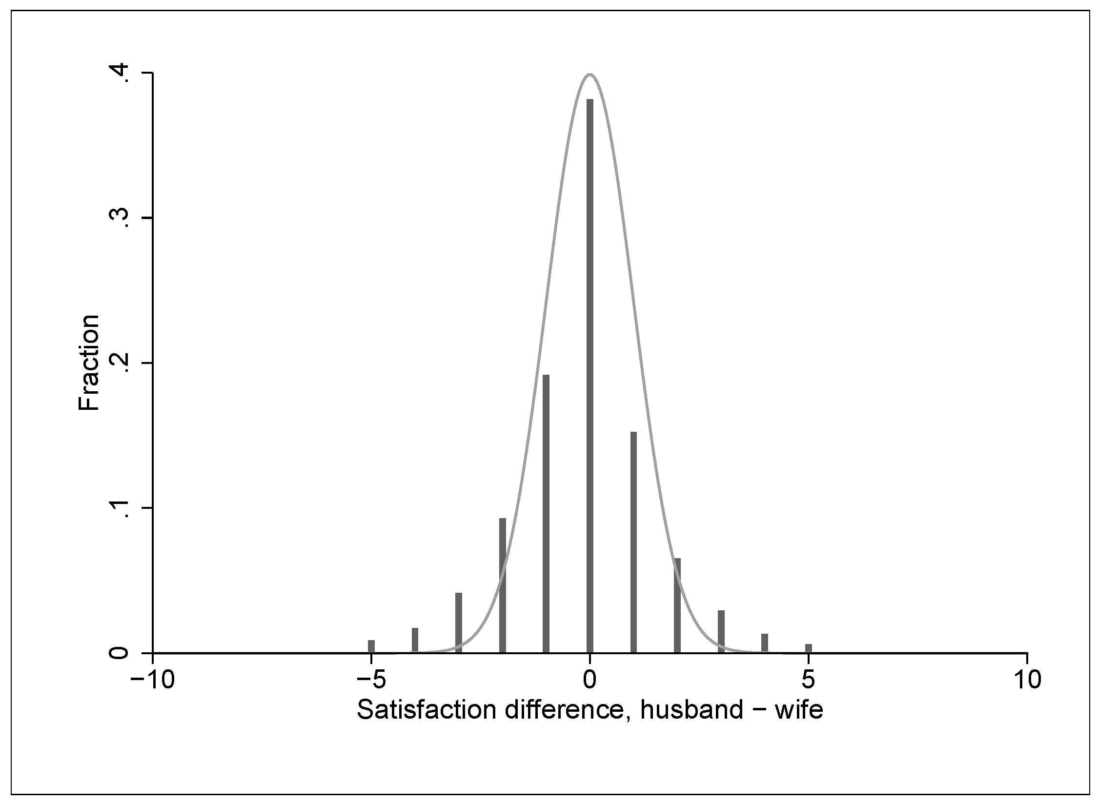
  • 12.While this variable could theoretically range from −10–10, its empirical range is −5–5.
  • 13.These include all monthly incomes at the time of the interview that do not depend on the household’s structure or income, e.g., no means-tested transfers, but, for example, different sorts of unemployment benefits, child benefits and widows’ pensions.
  • 14.Results are not shown here, though available on request.
  • 15.Information about the household income is one partner’s response to the question: “If you take a look at the total income from all members of the household: how high is the monthly household income today? Please state the net monthly income, which means after deductions for taxes and social security. Please include regular income such as pensions, housing allowance, child allowance, grants for higher education support payments, etc.”
  • 16.Couples where both partners are part-time or not employed (but not unemployed) and female breadwinner couples are too few for corresponding estimations.
  • 17.The z-value for the difference of the effects is z = δ 1 δ 2 s e ( δ 1 ) 2 + s e ( δ 2 ) 2 = 1 . 19 .
Figure 1. Differences in expressed financial satisfaction.
Socsci 05 00047 g001
Table 1. Sample mean and standard deviation of relevant variables.
VariableMeanSD 1 SD Within 2
Satisfaction difference−0.1371.5731.207
Men’s financial satisfaction6.3472.1311.154
Women’s financial satisfaction6.4842.1591.176
Men’s income3344.592582.311229.92
Women’s income1406.111524.81653.67
Income ratio0.7050.2440.112
Men’s working hours35.9819.459.584
Women’s working hours20.2418.218.579
Working hours ratio0.5860.3410.178
Equivalized household income 3 2007.771160.37586.36
Married0.893
Household without children0.377
Children under age of 6 in household0.211
Male breadwinner household 4 0.512
Partners equally employed0.303
Female breadwinner household 5 0.075
Households with at least one partner unemployed0.085
1 Standard deviation; 2 The within standard deviation describes the variation around the observation unit-specific mean, which is estimated as ( x i t x ¯ i ) 2 with x ¯ i being the observation unit’s mean; 3 Equivalized income is the monthly net household income, deflated with the square root of the household size; 4 The man is employed full-time, while the woman is part-time or not employed (though not unemployed); the man is working part-time, while the woman is not employed, though not unemployed; 5 The woman is employed full-time, while the man is part-time or not employed (though not unemployed); the woman is working part-time, while the man is not employed, though not unemployed. Source: SOEP 2012 [41], 36783 couple-year observations, 7573 couples.
Table 2. Determinants of differences in financial satisfaction and of financial satisfaction.
VariableDependent Variable: Satisfaction Difference Dependent Variable: Financial Satisfaction
Couples MenWomen
(1)(2)(3) (4)(5)
Coef. 1 SE 2 Coef. 1 SE 2 Coef. 1 SE 2 Coef. 1 SE 2 Coef. SE
Income ratio0.429***(0.119)0.443***(0.120)0.511***(0.116) −0.007 (0.123)−0.451***(0.126)
Working hours ratio 0.104 (0.093) 0.188**(0.094)0.084 (0.094)
Male breadwinner hh 4 , 5 -0.081 (0.052)
Female breadwinner hh 4 , 5 0.012 (0.063)
Other hh empl. situations 5 , 6 0.025 (0.064)
Man’s income−0.026**(0.012)−0.027**(0.012)−0.026**(0.012) 0.070***(0.014)0.097***(0.013)
Woman’s income0.011 (0.007)0.012 (0.007)0.010 (0.008) 0.012*(0.007)0.000 (0.008)
Man’s weekly working hours0.001 (0.001)−0.000 (0.002) 0.003*(0.002)0.003*(0.002)
Woman’s weekly working hours−0.002 (0.001)−0.001 (0.001) 0.003**(0.002)0.004***(0.001)
Man part-time empl. 3 −0.005 (0.051)
Woman part-time empl. 3 0.060 (0.055)
Man not employed 3 −0.048 (0.077)
Woman not employed 3 0.085 (0.068)
Youngest child up to 3 years 7 0.166*(0.093)0.162*(0.093)0.191**(0.093) 0.050 (0.091)−0.112 (0.091)
Youngest child 4–6 years 7 0.117 (0.090)0.116 (0.090)0.132 (0.091) 0.060 (0.090)−0.056 (0.089)
Youngest child 7–10 years 7 0.154*(0.088)0.153*(0.088)0.167*(0.088) 0.100 (0.087)−0.053 (0.087)
Youngest child 11–16 years 7 0.188**(0.082)0.187**(0.082)0.199**(0.083) 0.011 (0.081)−0.176**(0.083)
Yst. child older than 16 years 7 0.134*(0.071)0.132*(0.071)0.139*(0.071) −0.084 (0.072)−0.216***(0.073)
Monthly household income, log.0.106**(0.050)0.105**(0.050)0.110**(0.049) 1.314***(0.056)1.208***(0.056)
Household size, log.−0.332***(0.122)−0.332***(0.122)−0.329***(0.122) −0.569***(0.122)−0.237*(0.122)
Married0.115 (0.077)0.115 (0.077)0.119 (0.077) 0.090 (0.078)−0.025 (0.080)
Living in owned home0.072*(0.038)0.072*(0.038)0.073*(0.038) −0.025 (0.037)−0.098***(0.037)
Living in an urban area0.070 (0.060)0.070 (0.060)0.070 (0.060) 0.072 (0.058)0.002 (0.060)
Man unemployed−0.179***(0.055)−0.170***(0.055)−0.225***(0.062) −0.559***(0.061)−0.389***(0.059)
Woman unemployed0.107**(0.052)0.104**(0.052)0.133*(0.074) −0.249***(0.053)−0.353***(0.053)
Man’s self-rated health0.121***(0.014)0.121***(0.014)0.121***(0.014) 0.215***(0.015)0.094***(0.015)
Woman’s self-rated health−0.097***(0.015)−0.097***(0.015)−0.097***(0.015) 0.078***(0.013)0.176***(0.014)
Time fixed effectsyes yes yes yes yes
Constant−1.218***(0.414)−1.244***(0.414)−1.312***(0.418) −6.046***(0.462)−4.801***(0.466)
Linear regression estimations with household-specific fixed effects; Significance level: * <0.1, ** <0.05, *** <0.01; 1 Linear regression coefficient; 2 Robust standard errors, clustered by households; 3 Reference category: full-time employed; 4 Men/women employed at higher level (full-time vs. part-time, full-time vs. not employed, part-time vs. not employed), partner not unemployed; 5 Reference category: both partners working full-time, or both partners working part-time, or both partners not employed; 6 Couples with one or both partners unemployed; 7 Reference category: household without children. Source: SOEP 2012 [41]. i = 1 n t i = 36,783; n = 7573 .
Table 3. Subsample estimates.
Double Full-Time Male Breadwinner Household
(1) (2)(3)
Distribution factor
estimate, δ for
- couples1.988***(0.485) 1.257***(0.376)−0.235 (0.443)
- men1.299***(0.480) 0.204 (0.329)−0.657 (0.453)
- women−0.688 (0.468) −1.053***(0.379)−0.422 (0.404)
Estimate for the effect of
- man’s income
- on man’s SWHI0.010 (0.064) 0.117**(0.059)0.134***(0.047)
- on woman’s SWHI0.139**(0.063) 0.220***(0.060)0.092***(0.032)
- woman’s income
- on man’s SWHI0.124**(0.060) 0.015 (0.015)−0.010 (0.016)
- on woman’s SWHI0.047 (0.056) −0.012 (0.016)0.005 (0.015)
Subsample mean of
- man’s SWHI6.795 6.714 6.497
- woman’s SWHI6.887 6.847 6.646
- satisfaction difference−0.092 −0.133 −0.136
- income ratio0.556 0.757 0.929
n2525 3617 2436
N8065 11,737 7097
Linear regression estimations with individual-specific fixed effects; same specification as Model (2), (4) and (5) in Table 2, Robust standard errors, clustered by households, are in parentheses. Significance level: * <0.1, ** <0.05, *** <0.01, (1) Both partners full-time employed; (2) man full-time and women part-time employed; (3) man full- or part-time and women not employed, SWHI is satisfaction with household income. Source: SOEP 2012 [41].

