Contagion in the Euro Area Sovereign Bond Market

Abstract

In the last half-decade the European Monetary Union (EMU) has experienced a growing financial instability culminating with an extended sovereign debt crisis that has hit mostly the peripheral countries. Besides weak macroeconomic fundamentals, contagion phenomena in the government bond market damaged the countries more exposed to the financial stress. In this paper, the author investigates the issue of contagion applying to the financial field an innovative econometric technique, i.e., panel spatial regression. The paper documents: (i) the presence of contagion, in particular among peripheral countries; (ii) the changes in the magnitude of contagion in the different phases of the debt crisis; and (iii) the relevance of policy interventions in reducing the contagion effect in the EMU.

1. Introduction

The spectacular surge in the sovereign bond yield spreads in the peripheral countries of the EMU vis-á-vis to German Bunds after the explosion of the Greek debt crisis in the late 2009 have prompted research and policy interest on the causes of the debt crisis and contagion effects across European countries. Contagion effects can be a hint that investors are behaving irrationally (“herding behavior”) and not according to economic fundamentals or that transmission channels are not the responsibility of the affected country (e.g., balances sheets of international banks). However, contagion effects alone are not sufficient evidence in favor of a particular economic policy. Contagion can also be related to “wake-up-calls”. A “wake-up-call” is a situation where markets are “wrong” for some time and suddenly realize that some developments are not sustainable (e.g., long lasting high current account deficits). Nevertheless, information about contagion effects is of high relevance for the policy response in debt crisis.

There is no unanimous consensus on the definition of contagion, and the detection of the effect is dependent on its definition. In the literature there are three broad categories of definition. First, some authors interpret contagion as the co-movement in a variable of interest [1]. A second definition of contagion focuses on how the propagation mechanisms change after that an extreme shock occurs and compares this mechanism with pre-crisis period. Finally, a third group of authors focuses on spillover effects rather than contagion. Even if often the two terms are used vaguely, spillover refers to a lagged transmission of a shock, while contagion is simultaneous 1.

Our investigation will analyze jointly the behavior of yields spreads in 10 European countries. As we implement a study of the simultaneous effects across countries, we strictly focus on contagion and not on spillover. Our investigation fits at best with the first definition, indeed we are interested in disentangling whether the government bond spreads move jointly and whether the average effect changes from the pre-crisis period to the crisis. In this study we will focus only marginally on the propagation mechanisms of a such extreme shock.

The aim of this paper is to shed light on the existence of the contagion in the European sovereign bond markets applying an econometric methodology, panel spatial regression, that has been infrequently used for financial topics 2. Our methodology differs from the previous literature, where only the contagion effect generated from Greek spread is taken into account, by simultaneously modelling the reciprocal contagion of all countries in the monetary union. This research addresses some questions that are still the core of the academic and policy debate. The author will investigate the size of contagion in the government bond spreads, will track it in the different phases of the financial crisis and will compare the magnitude between two groups of countries: peripheral and core countries.

The remainder of the paper is organized as follows: in Section 2 the author will review the main literature in the field, in Section 3 the author will report a summary of the main events during the Eurozone crisis; in Section 4 the author will present the model; in Section 5 there will be an overview of the data used in the empirical analysis; Section 6 will present the empirical results; finally, Section 7 will conclude.

2. Literature Review

The withdraw of Greece from international bonds markets put intense pressure on other EMU countries with budget weaknesses like Ireland, Portugal, Spain and Italy. The weak fiscal conditions and the deep economic crises in these countries has led economic research to investigate the link between the movements in the bond spreads and the macroeconomic fundamentals. The main foundation of this branch of literature has been the market-based fiscal discipline hypothesis to determine the long-term government yields 3. In according to this hypothesis, markets ask higher premium to borrowers that borrow excessively. Indeed, the widening of government bond spread vis-á-vis to Germany was interpreted as an attempt by investors to diversify their sovereign debt portfolios to mitigate higher perceived country-risk. In the European context, where there is no integrated fiscal discipline, markets require a higher premium to countries with unsustainable fiscal positions. In Attinasi et al. [6], the authors apply a dynamic panel model estimation using FGLS technique adjusted for heteroskedasticity and autocorrelation and find a significant effect of budget positions, both deficit to GDP and debt to GDP ratios, on yield spreads. A bit in contrast, Barrios et al. [7] applying a time series analysis for selected European countries find that international factors, like the perceived risk, instead of national macroeconomic fundamentals play the major role in determining the bond spreads and domestic factors drive only little changes. Further, Aßmann and Boysen-Hogrefe [8] argue that the risk perception of market participants were time-varying and apply a time-varying coefficient approach 4.

In the current state of research, many authors claim that the spread in the peripheral countries were gripped by surges that are independent from the underlying macroeconomic fundamentals. This consideration has moved academic research to investigate the contagion effects across European countries. This second branch of literature developed theoretical models of contagion and tested empirically the size of this phenomenon in the EMU 5. In Bolton and Jeanne [14], the authors argue that sovereign contagion happens through integrated banking systems. In fact, under financial integration, banks diversify their holdings of sovereign debt to minimize the cost in case of default of an individual country. The diversification of sovereign debt generates risk diversification ex-ante and contagion ex-post. The authors find that, in the specific case of the EMU, the absence of integrated fiscal discipline leads to an inefficient equilibrium supply of government debt, i.e., the safest countries restrict the amount of sovereign debt issued, while the riskiest governments issue too much debt and do not foresee the consequences during crisis. In De Grauwe and Ji [13], the authors argue that the sovereign debt crisis in the EMU has to do with the essential feature of a monetary union. In other words, EU countries do not control the currency in which they issue their debts. The absence of the guarantee that cash will be always available when needed implies a systemic fragility of the monetary union and members are susceptible to movements of distrust. When investors fear liquidity problems, they sell government bonds, therefore, interest rates paid on bonds raise and budget problems are intensified. The ensuing liquidity crisis can degenerate into a solvency crisis. There is a self-fulfilling behavior; when investors fear default, they behave in such way that default becomes more likely. Under these circumstances, when distrust occurs, interest rates on government bonds rise affecting country solvency although macroeconomic fundamentals remain unchanged. To test empirically this theoretical prediction, the authors compare the results for the model with and without time dummies. The use of time dummies allows them to isolate movements in spreads that are unrelated to fundamentals and are caused by self-fulfilling effects. The authors find that the model with time dummies tracks the path of government bond spreads in the EMU, while the model without dummies fail to do it 6. Furthermore, they diversify for selected countries between the size of fundamentals and self-fulfilling effects and conclude that in Greece the jump in government bond spread was mostly caused by weak fundamentals, while in Spain, Italy and Belgium fundamentals explain only a little part of the movements in the national spreads. Arghyrou and Kontonikas [16] provide a model of the EMU crisis that combines features of both second- and third-generation approaches to currency crisis. Their main findings are in line with the previous literature, in fact they observe that market price for long-term government bonds is affected by both international risk and country specific fundamentals risk. The role of fundamentals is more significant during the crisis than in the period before the turmoil. Finally, they apply both time series and panel analysis and find in both cases that during the sovereign debt crisis the contagion from Greece was significant and damaged Spain, Portugal and Ireland, i.e., they report evidence that contagion was more pronounced for countries with weak fundamentals. In a recent paper, Canofari et al. [15] use game theory and cost-benefit analysis to determine when country-specific shocks are transmitted to other country members giving rise to contagion. In their model contagion occurs when the country-specific shock is large enough and above the threshold of staying in the monetary union. Furthermore, the authors implement a numerical simulation for the EMU countries and find that the Greek contagion was higher for Spain than for Italy. Contrary to the mainstream results, in Caporin et al. [3], the authors apply a Bayesian quantile regression approach to measure contagion in both CDS and government bond yield spreads and find that in the period post-Lehman Brothers there is no change in the intensity of transmission mechanism among European countries compared to the period before the collapse of the American bank.

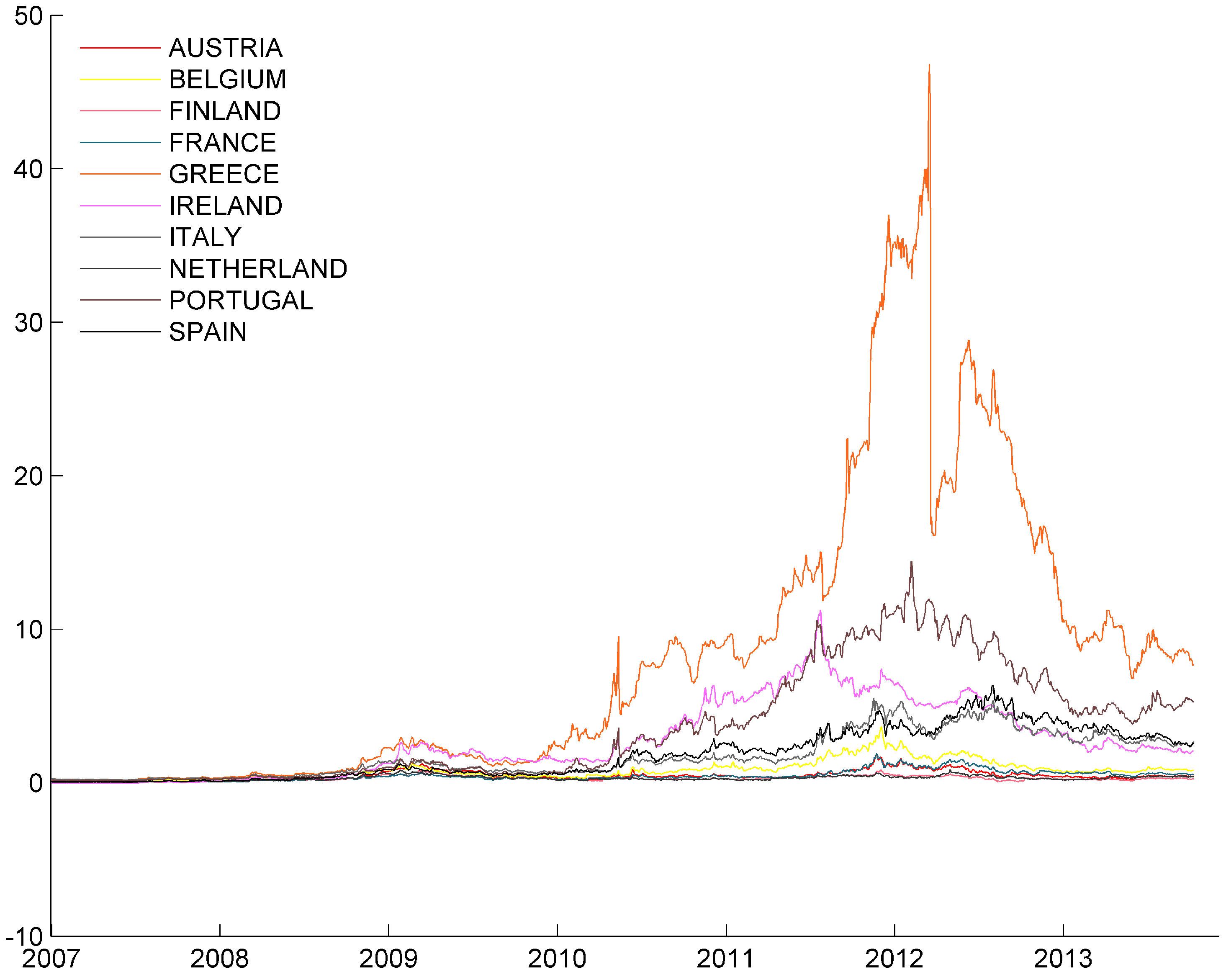
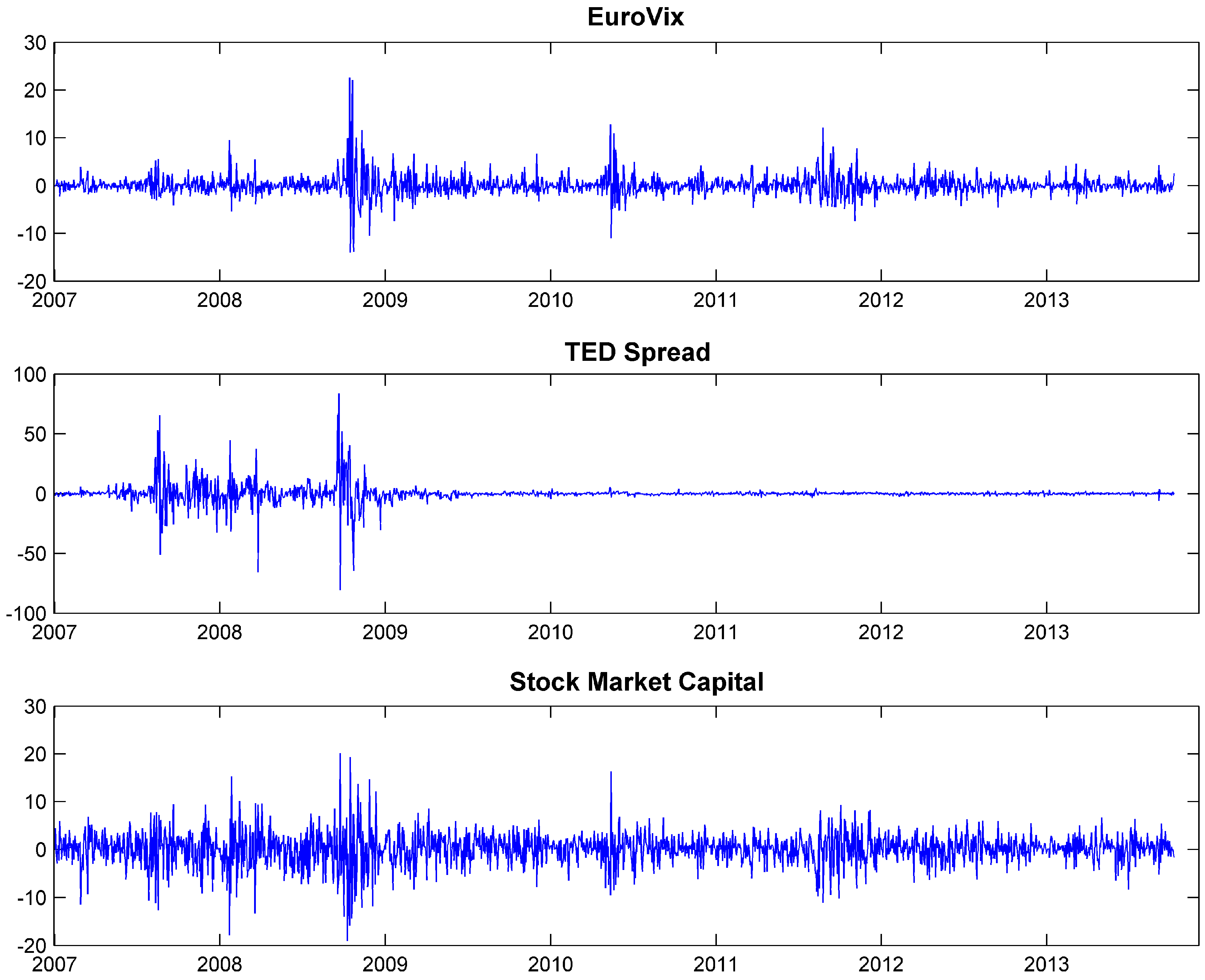
3. Stylized Facts about the Eurozone Crisis

In this Section the author will present a summary of the main events that have characterized the Eurozone crisis. A clear picture of the financial crisis is relevant to identify temporal breaking points in order to divide the period in sub-samples and to identify the countries that have been strongly hit by the sovereign debt crisis. Furthermore, a clear picture of the crisis allows the reader to better understand the mechanism of transmission of shocks and the weaknesses of the EMU.

From the creation of the EMU till the collapse of Lehman Brothers in September 2008 the spreads of all members of the Union vis-á-vis to the German Bund were very flat and close to zero. This indicates that investors did not perceive any country-specific risk among the EMU countries. In the pre-crisis phase the spread was very low despite of a gradual but constant deterioration of the macro-fundamentals in some peripheral countries. In the late 2008, after the bankruptcy of Lehman Brothers there was relatively low concern about the European sovereign debt. Due to the uncertainty created by the global financial crisis, investors reduced their international exposures. This reassessment of investment portfolio affected countries with large reliance on external funding. Concurrent with this portfolio reassessment, growth perspectives also declined due to the global recession and countries with weak fundamentals needed even a larger injection of external funding. In this phase we observe a deteriorating of the banking sector because of the overexposure of many banks toward unreliable debtors and because of low quality assets held in their balances. In the late 2009, the European sovereign debt crisis entered in a new phase. After the political elections in Greece, the official deficit to GDP ratios was much higher than expected. This unexpected shock joint with expected long-term recession and weakness of the banking system generated a vicious circle. These adverse developments were reflected in a spectacular surge of the government bond spreads not only in Greece but in all peripheral European countries like Ireland, Portugal, Spain and Italy. As noticed Arghyrou and Kontonikas [16], during the crisis the German Bund operated as “flight-to-quality”. Indeed, the 10-year German bond yield moved in the opposite direction of the general indicator of common international risk, the Chicago Board Options Exchange Volatility Index. This result indicates that in an uncertain environment investors flock to the perceived safety of the German Bund. This feature exacerbated further the turmoil in the government bond market in the peripheral countries. In Figure 1 the spreads of the European countries included in our analysis are shown for the period between 2007 and end of September 2013. We observe a general rise even if the magnitude of the jump is notably different from country to country. An important remark is that no EU country returned to its level of spreads before the beginning of the crisis. This result can have a twofold interpretations. In the case of “herding behavior”, this result would be a signal that the Union is still in a weak phase and additional reforms are needed. In the case of “wake-up-call”, different spread among the EMU countries higher than the pre-crisis period, would reflect the adjustments in the risk premium.

Figure 1. Government bond yields spreads.

Figure 1. Government bond yields spreads.

Note: Daily government bond yields between 2007 and 2013 for all countries in the sample are collected from DataStream. Spread relative to the German Bund are calculated by the author and plotted in the figure.

The escalation in the financial stress forced Greece to require financial assistance to the EU and IMF in May 2010; with Ireland following in November 2010 and Portugal in April 2011. A second rescue package was provided to Greece in March 2012 and in June Spain and Cyprus bow to bailout of their bank sector. In these bailouts official funding was provided on condition that the recipient would have implemented austerity measures and structural reforms to regain competitiveness on the international markets. In May 2010 joint with the rescue package provided to Greece, the EU set up the European Financial Stability Facility (EFSF) and the ECB launched the Security Market Programme (SMP) to buy Irish, Portuguese, Italian and Greek bonds over the next nine months. The unconventional measures adopted by the ECB to mitigate the contagion effect in the Eurozone and financially support countries under financial pressure continued in the second half of 2011, after the bailouts of Ireland and Portugal, with a second wave of SMP operations and then in July 2012, after the bailouts of Cyprus and Spain, with the launch of a new programme, the Outright Monetary Transactions (OMT) 7. The OMT differs from the SMP in four main respects: (1) the size of the OMT contrary to the SMP does not have an ex-ante quantitative limit; (2) the activation and continuation of the OMT is subject to strict and effective conditionality, while in the case of the SMP formally there was no strict conditionality to be matched; (3) contrary to the SMP, in the OMT the Eurosystem is treated pari passu with other creditors for the bonds purchased in the frame of this programme; (4) more transparency on OMT’s holdings is provided with respect to the SMP’s ones.

In 2013 the turmoil in the sovereign bonds market stabilized and the programmes adopted in 2012 achieved the first results. Together with this stabilization of the financial market, structural reforms, introduced in the first two-years of the crisis, continued to be implemented in all European countries. In particular, peripheral countries adopted reforms of the labor market and reviewed the public spending. At European level a centralized supervisor of the banking system was created to prevent dysfunctions of the banking sector as occurred at the origin of the debt crisis. In fact, the link between government bond crisis and weakness of the banking system was very clear at the origin of the crisis and had a twofold direction. Investors asked higher premium to countries after that extended a guarantee to their national banks, for example Ireland; on the other side, investors considered the increase of the sovereign risk as a negative impact for the national banks that held a large share of the government debt [14]. In addition to these structural reforms, the ECB opted for low interest rates to facilitate the economic recovery in the Eurozone. Although at the end of 2013 Eurozone countries faced an improvement of their current growth rates and of the forecasts for the following quarters, there is still a diffused uncertainty about the timing of complete economic recovery and fiscal consolidation of the Eurozone. This uncertainty arises many issues that policy-makers have to face in the forthcoming months. In fact, a slow recovery of the area may create serious problems of sustainability of the rescue packages worsening the living conditions in the peripheral countries, intensifying social inequalities and strengthening extreme positions against the monetary union 8.

4. Model

According to Elhorst [25], spatial panel data models are more informative than cross-sectional or panel model because they contain more variation and less collinearity across variables. Furthermore, another advantage of the spatial panel models is an higher number of degree of freedom and consequently an higher efficiency of the model. The basic idea of this approach is that panel observations are not independent and changes in a country’s conditions cause variations in the neighboring countries. The intensity of the contagion depends on the similarity between pair of countries in their economic structures. In standard spatial econometrics different functions of distances or common borders are used to link neighboring observations. In financial studies the geographic proximity is not a good proxy for similarity between two countries. Therefore, the first issue to deal with is the identification of a valid weight matrix. In this paper, I replicate the methodology suggested by Keiler and Eder [1]. The economic distance between pairs of countries is measured using correlations of the stock markets. The use of equity correlation may be problematic if a shock affects simultaneously both equity and bond markets. If that were the case, the distance matrix would be endogenous and statistical properties of the estimator would not hold. To solve this issue, the weight matrix is constructed by lagging the correlation by one year 9. An additional check on the weight matrix is needed. In fact, if the lagged stock market correlation contained information about the contemporary value of the government bond yields spread, the weight matrix would result endogenous also after lagging the correlation. To address this possibility, I calculate the correlation between the lagged equity returns and the government bond yields spread. The resulting value is very small and allows us to conclude that the weight matrix is exogenous and the statistical properties of the estimator are preserved 10.

Variables of interest in our analysis must be stationary. As panel unit root tests reject the stationarity of our series, all variables used in the empirical estimation are taken as first difference 11. Based on the previous considerations and with N that represents the number of cross-sectional observations in our sample and T the number of periods, the author tests a time-space simultaneous model with the following form:

$$\Delta {Govt}_t=\varphi \Delta {Govt}_{t-1}+\rho W\Delta {Govt}_t+X_t\beta +{ϵ}_t$$

(1)

$$E\left(ϵ\right)=0$$

(2)

$$E\left({ϵ}^{\prime }ϵ\right)={\alpha }^2{I}_N$$

(3)

where $\Delta {Govt}_t$ is a vector that includes the contemporary first difference in the government bond yields spread; $\Delta {Govt}_{t-1}$ is a vector cointains the lagged the first difference of the spread; W is the weight matrix of dimension $N\times N$; $X_t$ is the matrix of additional explanatory variables and finally ${ϵ}_t$ is a random (white noise) term 12. The additional regressors used as control variables are the first differences of the following indexes: (a) the EuroVix to control for financial turmoil as in Arghyrou and Kontonikas [16]; (b) the TED spread to control for the perceived risk in the global economy as in Gerlach et al. [27]; and finally (c) the total stock market index to control for market-wide business climate changes as in De Bruyckere et al. [28]. The model is estimated following a Maximum Likelihood procedure and using the Driscoll-Kraay estimator to account for robust error with cross-sectional dependence. The advantage of a panel data structure is that enables us to analyze a phenomenon that happens over time. The inclusion in the model of spatial specific effects allows us to account for local heterogeneity that is assumed to remain constant over time. In our specific case, this assumption sounds very reasonable because we focus on a short period of time. The exclusion of country specific effects may determine biased and ineffcient estimators.

By applying such a methodology, we address the question of how on average the government bond spread of a country in the European Union depends on the government bonds spread of all other countries in the Union. If we find that there is a significant effect on a country of the government bond spreads of all other countries, this constitutes evidence of financial contagion. Consequently, such a model allows us to measure and test for the presence of contagion effects in the European Union.

5. Data

Data on government bond yields are downloaded from DataStream with daily frequency for the period from January 2007 to end of Septembet 2013. The spread in yields is calcuated vis-á-vis to the German government bond yield. The dynamics of the country specific spreads over the period of study are shown in Figure 1.

In our empirical investigation we test whether the size of the spatial correlation vary in the different phases of the crisis and between two groups of countries, the peripheral and the core ones. To implement this further investigation we need to divide our period of analysis in sub-periods. Based on the overview of the main events during the crisis in Section 3 the author opted to divide the period in five distinct sub-periods. The first sub-period is the pre-crisis period and goes from 2007 to the collapse of Lehman Brothers; the second sub-period is the subprime crisis period and is between the collapse of Lehman Brothers and the announcement of a much higher Greek deficit than expected; the third phase is the Greek Debt crisis and it ends with the announcement of S&P that 15 countries in the Eurozone are under revision, i.e., when the crisis turns to spread across the Euro area; the fourth sub-period is the European sovereign debt crisis and it ends with the promulgation of the OMT in July 2012; the last sub-period is characterized by the ECB interventions and policy-makers reforms and goes till the end of the period of study. The countries in the sample are divided in two sub-groups, the first sub-group includes countries that have been strongly hit by the sovereign debt crisis, while the second one contains the countries that have faced a lower intensity of financial turmoil. Precisely, the highly exposed countries to the financial stress are the peripheral countries: Greece, Portugal, Ireland, Spain and Italy, while the low exposed countries are the core countries are France, Belgium, Netherlands, Finland and Austria13.

Table 1 shows the average standard deviation and autocorrelation of government bond spreads by temporal sub-periods and country sub-groups. First of all, we note that the standard deviation of the government bond spreads has an inverse U-shape form. Differences in spreads are very low before the financial crisis, after the explosion first of the US financial crisis and then of the EMU sovereign debt crisis standard deviations increase and reach their peak in the fourth sub-period, the one in which the contagion among EMU countries is more marked. Second, although the inverse U-shape form is observed for both highly and low exposed countries, the latter have on average lower standard deviation. Third, we observe that the highest difference between the standard deviation of the two sub-groups is in the fourth sub-period (54.16 percentage points). Fourth, the decrease of the standard deviation in the fifth sub-period, joint with the lowering of the average spreads as noticed in Figure 1, is a positive signal of the success of the stabilizing policy measures implemented by the ECB. Turn to the average autocorrelation, the path is comparable to the one of the standard deviation. Two main features have to be highlighted. First, contrary to the standard deviation the peak is reached in the third sub-period; second the autocorrelation turns to be negative in the first sub-period and positive afterwards.

Table 1. Descriptive statistics.

	All Countries	Highly Exposed	Low Exposed
Entire Sample
Standard Deviation (%)	13.31	23.6	3.02
Autocorrelation	0.16	0.21	0.12
First Subsample
Standard Deviation (%)	0.54	0.62	0.45
Autocorrelation	–0.02	–0.04	–0.01
Second Sub-sample
Standard Deviation (%)	2.9	3.81	1.98
Autocorrelation	0.22	0.29	0.15
Third Sub-sample
Standard Deviation (%)	11.66	19.54	3.77
Autocorrelation	0.18	0.24	0.13
Fourth Sub-sample
Standard Deviation (%)	32.04	59.12	4.96
Autocorrelation	0.12	0.16	0.08
Firth Sub-sample
Standard Deviation (%)	7.89	13.4	2.37
Autocorrelation	0.12	0.2	0.03

Note: Daily series for the government bond yields are downloaded from DataStream for all countries in the sample. The average standard deviation and autocorrelation across countries are calculated by the author. Statistics are divided in temporal sub-samples based on the classification mentioned above in the paper.

Table 1. Descriptive statistics.

	All Countries	Highly Exposed	Low Exposed
Entire Sample
Standard Deviation (%)	13.31	23.6	3.02
Autocorrelation	0.16	0.21	0.12
First Subsample
Standard Deviation (%)	0.54	0.62	0.45
Autocorrelation	–0.02	–0.04	–0.01
Second Sub-sample
Standard Deviation (%)	2.9	3.81	1.98
Autocorrelation	0.22	0.29	0.15
Third Sub-sample
Standard Deviation (%)	11.66	19.54	3.77
Autocorrelation	0.18	0.24	0.13
Fourth Sub-sample
Standard Deviation (%)	32.04	59.12	4.96
Autocorrelation	0.12	0.16	0.08
Firth Sub-sample
Standard Deviation (%)	7.89	13.4	2.37
Autocorrelation	0.12	0.2	0.03

Note: Daily series for the government bond yields are downloaded from DataStream for all countries in the sample. The average standard deviation and autocorrelation across countries are calculated by the author. Statistics are divided in temporal sub-samples based on the classification mentioned above in the paper.

Data on EuroVix, TED spread and total stock market index are collected with daily frequency from DataStream. In Figure 2 the daily changes of the additional variables are plotted. The first subplot shows the EuroVix Index. We observe three distinct waves of strong financial market volatility in the Euro area. These three jumps are linked to the three main shocks that hit the EMU in the last years. The first shock is in the late 2008 after the collapse of Lehman Brothers. This shock caused a global rise in uncertainty and risk. In fact, from the second subplot, that reports the TED spread, we observe a global worsening of the perceived risk. The massive jump after the events of mid-September 2008 was preceded by pre-crisis adjustments of the perceived risks since the first half of 2007. The second and third jumps in the EuroVix affected exclusively the Eurozone, indeed we observe a very pronounced flatness of the TED spread for the period following the US subprime crisis. This evidence highlights the fact that the second two jumps in the EuroVix are due to local shocks that can be linked with the Greek sovereign debt crisis and Portugal bailouts, respectively. An interesting finding is that investors seem not to strongly react to the Spanish bailout. Likely, investor do not overreact to the Spanish events because they were prepared to this eventuality and gradually adjusted their risk premium.

Figure 2. Additional regressors for the empirical analysis.

Figure 2. Additional regressors for the empirical analysis.

Note: Daily volatility for the Euro area (VIX Index), daily TED spreads and daily total stock market index between 2007 and end September 2013 are collected from Bloomberg. Averages across countries are plotted in the figure.

The third subplot of Figure 2 adds interesting elements to the European economic picture. This subplot shows the first difference in the daily total stock market capital index. The first feature that we observe is a much higher volatility than the other two indexes. As already mentioned above, changes in the stock market capital index are good proxies for changes in the economic-wide business environment in the Euro area. The high volatility suggests that in the last years there was a large uncertainty among financial operators about the real economic conditions and perspective of the Union. This result is not surprising, in fact the existence of panic and disorientation in the European financial markets is a common finding in the literature.

6. Empirical Results

Empirical results of model (1) are shown in Table 2 for countries highly exposed to the sovereign debt crisis and in Table 3 for countries not highly hit by the debt crisis. In Table 4, I show the results for countries highly exposed to the sovereign debt crisis excluding Greece and finally, in Table 5 the results for the sample including all countries are presented.

In our analysis the most important coefficient is ρ that measures the spatial correlation, representing the situation where the dependent variable observed for each country is determined jointly with that of its neighbors. The significance of the coefficient ρ implies that on average a change in spread in the neighbouring countries have a significant positive impact on domestic change in spread. The estimates in column (1) of Table 2 and Table 3 are both positive and significant. Therefore, we can conclude that in both country sub-groups the spatial dimension is relevant and the positive sign of the coefficient implies changes in spread commoved together in the period of study. The next step is to test whether the model selection is appropiate. Basically, we have to test the existence of spatial relationship. To test the existence of the spatial dependence, the Lagrangian Multiplier Test is reported at the bottom of each column 14. The test compare the null hypothesis of no spatial effect $\left(\rho =0\right)$ versus the alternative hypothesis of existence of spatial dependence $\left(\rho \ne 0\right)$. The pvalues in column (1) of Table 2 and Table 3 are very low. Therefore, we reject the null hypothesis and we can conclude that there is evidence of the existence of spatial dependence. Before moving to the sub-periods analysis, a brief comment on the $R^2$ is needed. First, $R^2$ is an inappropriate measure of fit in spatial econometrics because is based on the unweighted sum of squared residuals. That is the reason why the interpretation in presence of spatial effects may be misleading. Second, focusing on the reported values for the $R^2$, we notice that they are relatively low. This result is not surprising, indeed our findings are very much in line with the literature that uses the first differences of the variables of interest as dependent and explanatory variables. Third, low pvalues would be problematic in our findings only if they hinted the presence of omitted variables. That does not seem to be the case for two reasons: first, we use country specific fixed effects dummies to control for all unobserved variables; second, the variables used in our model are the ones widely applied in the literature. In addition to the results for the spatial coefficient, we observe that while the lagged yields spread has a significant impact for both sub-groups of countries over the entire period, the additional explanatory variables—Risk, TED Spread and Market Capitalization—are not very important drivers of changes in spread, indeed they turn to be always non-significant.

Table 2. Empirical results for highly exposed countries to the sovereign debt crisis.

	(1)	(2)	(3)	(4)	(5)	(6)
	Entire	I	II	III	IV	V
Main
Lag Yields Spread	0.10	0.03	0.16 ***	0.20 **	0.07	0.22 ***
Risk	0.00	0.00	0.00	0.00	0.01	0.00
TED Spread	0.00	0.00	0.00	0.00	0.00	0.00 *
Market Capitalization	0.00	0.00	0.00	0.00	–0.01	0.00
Spatial ρ	0.12 *	0.50 ***	0.61 ***	0.41 ***	0.02	0.44 ***
Observations	8800	915	1730	3760	860	1510
Number of Countries	5	5	5	5	5	5
RSquare	0.01	0.01	0.09	0.06	0.01	0.07
Pvalues LM-Test	0.00	0.00	0.00	0.00	0.90	0.00

Note: In the table are reported the results for the model in Equation (1) for the most exposed countries to the European sovereign debt crisis: Greece, Portugal, Ireland, Spain and Italy. The model is estimated for different temporal sub-samples in according to the above division of the sample. The model is estimated via Maximum Likelihood estimator using a Driscoll-Kraay robust estimator and country fixed effects. Significance Levels: * 0.1, ** 0.05, *** 0.001.

Table 2. Empirical results for highly exposed countries to the sovereign debt crisis.

	(1)	(2)	(3)	(4)	(5)	(6)
	Entire	I	II	III	IV	V
Main
Lag Yields Spread	0.10	0.03	0.16 ***	0.20 **	0.07	0.22 ***
Risk	0.00	0.00	0.00	0.00	0.01	0.00
TED Spread	0.00	0.00	0.00	0.00	0.00	0.00 *
Market Capitalization	0.00	0.00	0.00	0.00	–0.01	0.00
Spatial ρ	0.12 *	0.50 ***	0.61 ***	0.41 ***	0.02	0.44 ***
Observations	8800	915	1730	3760	860	1510
Number of Countries	5	5	5	5	5	5
RSquare	0.01	0.01	0.09	0.06	0.01	0.07
Pvalues LM-Test	0.00	0.00	0.00	0.00	0.90	0.00

Note: In the table are reported the results for the model in Equation (1) for the most exposed countries to the European sovereign debt crisis: Greece, Portugal, Ireland, Spain and Italy. The model is estimated for different temporal sub-samples in according to the above division of the sample. The model is estimated via Maximum Likelihood estimator using a Driscoll-Kraay robust estimator and country fixed effects. Significance Levels: * 0.1, ** 0.05, *** 0.001.

Table 3. Empirical results for low exposed countries to the sovereign debt crisis.

	(1)	(2)	(3)	(4)	(5)	(6)
	Entire	I	II	III	IV	V
Main
Lag Yields Spread	0.12 ***	0.00	–0.05	0.16 ***	0.08 **	0.03
Risk	0.00	0.00	0.00	0.00	0.00	0.00 *
TED Spread	0.00	0.00	0.00	0.00	0.00	0.00
Market Capitalization	0.00	0.00	0.00	0.00	0.00	0.00
Spatial ρ	0.54 ***	0.46 ***	0.58 ***	0.55 ***	0.56 ***	0.54 ***
Observations	8800	915	1730	3760	860	1510
Number of Countries	5	5	5	5	5	5
RSquare	0.03	0.01	0.01	0.05	0.02	0.01
Pvalues LM-Test	0.00	0.00	0.00	0.00	0.00	0.00

Note: In the table are reported the results for the model in Equation (1) for the least exposed countries to the European sovereign debt crisis: France, Belgium, Netherlands, Finland and Austria. The model is estimated for different temporal sub-samples in according to the above division of the sample. The model is estimated via Maximum Likelihood estimator using a Driscoll-Kraay robust estimatorand country fixed effects. Significance Levels: * 0.1, ** 0.05, *** 0.001.

Table 3. Empirical results for low exposed countries to the sovereign debt crisis.

	(1)	(2)	(3)	(4)	(5)	(6)
	Entire	I	II	III	IV	V
Main
Lag Yields Spread	0.12 ***	0.00	–0.05	0.16 ***	0.08 **	0.03
Risk	0.00	0.00	0.00	0.00	0.00	0.00 *
TED Spread	0.00	0.00	0.00	0.00	0.00	0.00
Market Capitalization	0.00	0.00	0.00	0.00	0.00	0.00
Spatial ρ	0.54 ***	0.46 ***	0.58 ***	0.55 ***	0.56 ***	0.54 ***
Observations	8800	915	1730	3760	860	1510
Number of Countries	5	5	5	5	5	5
RSquare	0.03	0.01	0.01	0.05	0.02	0.01
Pvalues LM-Test	0.00	0.00	0.00	0.00	0.00	0.00

Note: In the table are reported the results for the model in Equation (1) for the least exposed countries to the European sovereign debt crisis: France, Belgium, Netherlands, Finland and Austria. The model is estimated for different temporal sub-samples in according to the above division of the sample. The model is estimated via Maximum Likelihood estimator using a Driscoll-Kraay robust estimatorand country fixed effects. Significance Levels: * 0.1, ** 0.05, *** 0.001.

Table 4. Empirical results for highly exposed countries to the sovereign debt crisis excluding Greece.

	(1)	(2)	(3)	(4)	(5)	(6)
	Entire	I	II	III	IV	V
Main
Lag Yields Spread	0.21 ***	–0.01	0.15 ***	0.18 ***	0.26 ***	0.13 ***
Risk	0.00	0.00	0.00	0.00	0.00	0.00
TED Spread	0.00	0.00	0.00	0.00	0.00	0.00 **
Market Capitalization	0.00 *	0.00	0.00	0.00	0.00	0.00
Spatial ρ	0.43 ***	0.39 ***	0.57 ***	0.47 ***	0.28 ***	0.50 ***
Observations	7040	732	1384	3008	688	1208
Number of Countries	4	4	4	4	4	4
RSquare	0.06	0.01	0.08	0.07	0.07	0.05
Pvalues LM-Test	0.00	0.00	0.00	0.00	0.00	0.00

Note: In the table are reported the results for the model in Equation (1) for the most exposed countries to the European sovereign debt crisis: Portugal, Ireland, Spain and Italy. The model is estimated for different temporal sub-samples in according to the above division of the sample. The model is estimated via Maximum Likelihood estimator using a Driscoll-Kraay robust estimator and country fixed effects. Significance Levels: * 0.1, ** 0.05, *** 0.001.

Table 4. Empirical results for highly exposed countries to the sovereign debt crisis excluding Greece.

	(1)	(2)	(3)	(4)	(5)	(6)
	Entire	I	II	III	IV	V
Main
Lag Yields Spread	0.21 ***	–0.01	0.15 ***	0.18 ***	0.26 ***	0.13 ***
Risk	0.00	0.00	0.00	0.00	0.00	0.00
TED Spread	0.00	0.00	0.00	0.00	0.00	0.00 **
Market Capitalization	0.00 *	0.00	0.00	0.00	0.00	0.00
Spatial ρ	0.43 ***	0.39 ***	0.57 ***	0.47 ***	0.28 ***	0.50 ***
Observations	7040	732	1384	3008	688	1208
Number of Countries	4	4	4	4	4	4
RSquare	0.06	0.01	0.08	0.07	0.07	0.05
Pvalues LM-Test	0.00	0.00	0.00	0.00	0.00	0.00

Note: In the table are reported the results for the model in Equation (1) for the most exposed countries to the European sovereign debt crisis: Portugal, Ireland, Spain and Italy. The model is estimated for different temporal sub-samples in according to the above division of the sample. The model is estimated via Maximum Likelihood estimator using a Driscoll-Kraay robust estimator and country fixed effects. Significance Levels: * 0.1, ** 0.05, *** 0.001.

Table 5. Empirical results for the entire sample of EMU countries.

	(1)	(2)	(3)	(4)	(5)	(6)
	Entire	I	II	III	IV	V
Main
Lag Yields Spread	0.10	0.03	0.16 ***	0.20 **	0.07	0.22 ***
Risk	0.00	0.00	0.00	0.00	0.01	0.00
TED Spread	0.00	0.00	0.00	0.00	0.00	0.00 *
Market Capitalization	0.00	0.00	0.00	0.00	–0.01	0.00
Spatial ρ	0.12 *	0.50 ***	0.61 ***	0.41 ***	0.02	0.44 ***
Observations	17,600	1830	3460	7520	1720	3020
Number of Countries	10	10	10	10	10	10
RSquare	0.01	0.01	0.06	0.06	0.01	0.06
Pvalues LM-Test	0.00	0.00	0.00	0.00	0.69	0.00

Note: In the table are reported the results for the model in Equation (1) for the EMU countries in the sample. The model is estimated for different temporal sub-samples in according to the above division of the sample. The model is estimated via Maximum Likelihood estimator using a Driscoll-Kraay robust estimator and country fixed effects. Significance Levels: * 0.1, ** 0.05, *** 0.001.

Table 5. Empirical results for the entire sample of EMU countries.

	(1)	(2)	(3)	(4)	(5)	(6)
	Entire	I	II	III	IV	V
Main
Lag Yields Spread	0.10	0.03	0.16 ***	0.20 **	0.07	0.22 ***
Risk	0.00	0.00	0.00	0.00	0.01	0.00
TED Spread	0.00	0.00	0.00	0.00	0.00	0.00 *
Market Capitalization	0.00	0.00	0.00	0.00	–0.01	0.00
Spatial ρ	0.12 *	0.50 ***	0.61 ***	0.41 ***	0.02	0.44 ***
Observations	17,600	1830	3460	7520	1720	3020
Number of Countries	10	10	10	10	10	10
RSquare	0.01	0.01	0.06	0.06	0.01	0.06
Pvalues LM-Test	0.00	0.00	0.00	0.00	0.69	0.00

Note: In the table are reported the results for the model in Equation (1) for the EMU countries in the sample. The model is estimated for different temporal sub-samples in according to the above division of the sample. The model is estimated via Maximum Likelihood estimator using a Driscoll-Kraay robust estimator and country fixed effects. Significance Levels: * 0.1, ** 0.05, *** 0.001.

Turning to the sub-periods we obtained two main findings: first, the coefficient for the highly exposed countries is more volatile across sub-periods than in the low exposed countries; second, while in the low exposed countries the coefficient is always significant at 1% level, in the highly exposed countries turns to be non-significant in the fourth sub-period. A possible explanation for this finding is that the jump in the Greek yield spread was abnormal and incomparable with any other European country. The inclusion of Greece in the sample may be a source of bias for the overall result in the analysis of the highly exposed countries. To check the importance of the Greek impact on our findings, we run the model in Equation (1) excluding Greece. Results are reported in Table 4. The spatial coefficient turn to be positive and highly significant for the entire period and in each sub-period. This finding implies that the Greek abnormal yields spread, due to a jump in the risk of country default, has an huge impact in the estimation. Indeed, the behavior of the spreads in the remaining countries is more similar and this is the reason why we observe stronger co-movements. The coefficients of the control variables are only slightly affected by the exclusion of Greece. In the remaining part of the paper, I will refer to the results of Table 4 as results for the highly exposed countries.

A deeper look at the estimates for the other explanatory variables highlights that the control variables are mostly non-significant except for Risk in the fifth sub-period for the low exposed countries and TED spread in the same sub-period for the highly exposed countries significant at the 10% and at the 5% levels, respectively. In all cases, the coefficient show a positive sign in line with our theoretical expectations. Indeed, an increase in risk will determine a jump in the yields spread as well as an increase in the perceived credit risk associated with the global economy will lead to a rise in the yields differential. The main differences between the two groups of countries are observed in the lagged yields spread. While in the highly exposed countries lagged spread is significant at 1% level for the entire period and in each sub-period except the first one, in the low exposed countries the lagged yields spread is significant only in the central phases of the debt crisis, i.e., in the third and fourth sub-periods. This finding shows how in period of financial distress investors rely strongly on the past performance of the spread to assess the level of today’s spread. This finding holds in particular for those countries that are more exposed to financial turmoil.

Overall our results evidence the relevance of the lagged spread in determining the current change and highlight that the cross-countries trasmission of these effects is very significant in all pahses of the crisis and for both countries sub-groups. This finding is interpreted as evidence of contagion across Euroepan countries.

7. Conclusions

In this paper we investigate the presence of contagion effects in the Eurozone in the period from 2007 to September 2013 and in particular in the period after the announcement of OMT. The contagion in the government bonds spread market in the Eurozone has become an important topic of the academic and political debate. A visual inspection of the sovereign debt movements emphasizes co-movements in the country spreads in the peripheral region of the Union. A few theoretical works suggested different mechanisms how the contagion occurs and how it propagates in a monetary Union. A few empirical studies have focused on quantifying the magnitude of the contagion. This branch of literature is very limited and results are controversial. The contribution of this paper to the literature is to identify the contagion applying an econometric methodology that is not widely applied in the field, i.e., panel spatial regression. The time-space simultaneous model shows that the spatial coefficient is strongly significant in all five sub-period and both country groups, the peripheral and the core countries of the Union. The model points out also the importance for investors of the lagged yields spread in period of financial turmoil.

In fact, the magnitude of the coefficient of the lagged spread is drastically decreasing in the last phase of the crisis, turning even non-significant for the low exposed countries, due to the policy interventions that decrease the uncertainty in the market. In conclusion, the methodology returns robust evidence on the existence of contagion in the Eurozone and on the importance of policy interventions to alleviate the consequences of this phenomenon. Further research is needed to better understand the channels of contagion and the causes of it in the Euroarea.

References

1. Sebastian Keiler, and Armin Eder. “CDS spreads and systemic risk: A spatial econometric approach.” Discussion Papers 01/2013. Frankfurt am Main, Germany: Deutsche Bundesbank, Research Centre, 2013. [Google Scholar]
2. Carmen Broto, and Gabriel Perez-Quiros. “Disentangling Contagion among Sovereign CDS Spreads during the European Debt Crisis.” Banco de Espana Working Papers 1314. Madrid, Spain: Banco de Espana, 2013. [Google Scholar]
3. Massimiliano Caporin, Loriana Pelizzon, Francesco Ravazzolo, and Roberto Rigobon. “Measuring Sovereign Contagion in Europe.” NBER Working Papers 18741. Cambridge, MA, USA: National Bureau of Economic Research, 2013. [Google Scholar]
4. Ari Tjahjawandita, Tito Pradono, and Rullan Rinaldi. “Spatial Contagion of Global Financial Crisis.” Working Papers in Economics and Development Studies (WoPEDS) 200906. Bandung, Indonesia: Department of Economics, Padjadjaran University, August 2009. [Google Scholar]
5. Morris Goldstein, and Geoffrey Woglom. “Market-Based Fiscal Discipline in Monetary Unions: Evidence from the U.S. Municipal Bond Market.” IMF Working Papers 91/89. Washington, DC, USA: International Monetary Fund, 1991. [Google Scholar]
6. Maria-Grazia Attinasi, Cristina Checherita, and Christiane Nickel. “What Explains the Surge in Euro Area Sovereign Spreads during the Financial Crisis of 2007-09.” Working Paper Series 1131. Frankfurt am Main, Germany: European Central Bank, 2009. [Google Scholar]
7. Salvador Barrios, Per Iversen, Magdalena Lewandowska, and Ralph Setzer. “Determinants of intra-euro area government bond spreads during the financial crisis.” European Economy-Economic Papers 388. Brussels, Belgium: Directorate General Economic and Monetary Affairs (DG ECFIN), European Commission, 2009. [Google Scholar]
8. Christian Aßmann, and Jens Boysen-Hogrefe. “Determinants of government bond spreads in the Euro area: In good times as in bad.” Empirica 39 (2012): 341–56. [Google Scholar] [CrossRef]
9. Niko Doetz, and Christoph Fischer. “What can EMU Countries’ Sovereign Bond Spreads Tell Us about Market Perceptions of Default Probabilities during the Recent Financial Crisis? ” Discussion Paper, Series 1: Economic Studies, No. 11/2010. Frankfurt am Main, Germany: Deutsche Bundesbank, Research Centre, 2010. [Google Scholar]
10. Carlos Caceres, Vincenzo Guzzo, and Miguel Segoviano. “Sovereign Spreads: Global Risk Aversion, Contagion or Fundamentals? ” IMF Working Papers 10/120. Washington, DC, USA: International Monetary Fund, 2010. [Google Scholar]
11. In-Mee Baek, Arindam Bandopadhyaya, and Chan Du. “Determinants of market-assessed sovereign risk: Economic fundamentals or market risk appetite? ” Journal of International Money and Finance 24 (2005): 533–48. [Google Scholar] [CrossRef]
12. David Haugh, Patrice Ollivaud, and David Turner. “What Drives Sovereign Risk Premiums?: An Analysis of Recent Evidence from the Euro Area.” OECD Economics Department Working Papers 718. Paris, France: OECD Publishing, 2009. [Google Scholar]
13. Paul De Grauwe, and Yuemei Ji. “Self-fulfilling crises in the Eurozone: An empirical test.” Journal of International Money and Finance 34 (2013): 15–36. [Google Scholar] [CrossRef]
14. Patrick Bolton, and Olivier Jeanne. “Sovereign Default Risk and Bank Fragility in Financially Integrated Economies.” NBER Working Papers 16899. Cambridge, MA, USA: National Bureau of Economic Research, 2011. [Google Scholar]
15. Paolo Canofari, Giovanni Di Bartolomeo, and Piersantii Giovanni. “Theory and practice of contagion in monetary unions. Domino effects in EU Mediterranean countries: The case of Greece, Italy and Spain.” International Advances in Economic Research 20 (2013): 259–67. [Google Scholar] [CrossRef]
16. Michael Arghyrou, and Alexandros Kontonikas. “The EMU sovereign-debt crisis: Fundamentals, expectations and contagion.” Journal of International Financial Markets, Institutions and Money 22 (2012): 658–77. [Google Scholar] [CrossRef]
17. Paul De Grauwe. “Governance of a fragile Eurozone.” CEPR Working Paper 346. Brussels, Belgium: Centre for European Policy Studies, 4 May 2011. [Google Scholar]
18. Marta Gomez-Puig, and Simon Sosvilla-Rivero. “Causality and contagion in peripheral EMU public debt markets: A dynamic approach.” Working Papers 11-06. Valladolid, Spain: Asociacion Espanola de Economia y Finanzas Internacionales, 2011. [Google Scholar]
19. Norbert Metiu. “Sovereign risk contagion in the Eurozone.” Economics Letters 117 (2012): 35–38. [Google Scholar] [CrossRef]
20. Mark Mink, and Jakob de Haan. “Contagion during the Greek sovereign debt crisis.” Journal of International Money and Finance 34 (2013): 102–13. [Google Scholar] [CrossRef]
21. Jurgen Von Hagen, Ludger Schuknecht, and Guido Wolswijk. “Government bond risk premiums in the EU revisited: The impact of the financial crisis.” European Journal of Political Economy 27 (2011): 36–43. [Google Scholar] [CrossRef]
22. Roberto De Santis. “The Euro Area Sovereign Debt Crisis: Identifying Flight-to-Liquidity and the Spillover Mechanisms.” Journal of Empirical Finance 26 (2014): 150–70. [Google Scholar] [CrossRef]
23. Matteo Falagiarda, and Stefan Reitz. “Announcements of ECB Unconventional Programs: Implications for the Sovereign Risk of Italy.” Kiel Working Papers 1866. Kiel, Germany: Institute for the World Economy, 2013. [Google Scholar]
24. Philip R. Lane. “The European Sovereign Debt Crisis.” Journal of Economic Perspectives 26 (2012): 49–68. [Google Scholar] [CrossRef]
25. J. Paul Elhorst. “Spatial panel data models.” In Handbook of Applied Spatial Analysis. Edited by Fischer Manfred and Getis Arthur. New York: Springer, 2010, pp. 377–407. [Google Scholar]
26. Luc Anselin, Raymond Florax, and Sergio J. Rey. Advances in Spatial Econometrics: Methodology, Tools and Applications. New York: Springer, 2004. [Google Scholar]
27. Stefan Gerlach, Alexander Schulz, and Wolff B. Guntram. “Banking and sovereign risk in the euro area.” Discussion Paper, Series 1: Economic Studies, No. 9/2010. Frankfurt am Main, Germany: Deutsche Bundesbank, Research Centre, 2010. [Google Scholar]
28. Valerie De Bruyckere, Maria Gerhardt, Glenn Schepens, and Rudi Vander Vennetb. “Bank/sovereign risk spillovers in the European debt crisis.” Working Paper Research 232. Brussels, Belgium: National Bank of Belgium, 2012. [Google Scholar]
29. Luc Anselin, Julie Le Gallo, and Hubert Jaynet. Spatial Panel Econometric. New York: Springer, 2008. [Google Scholar]
• 1For an extensive discussion on these issue, see [2] and [3]
• 2For additional references on the application of this methodology to financial issues, see [1,4].
• 3For an extensive discussion on these issue, see [5].
• 4For additional references on these issues, see [9,10,11,12].
• 5The main contributions to this branch of the literature are [13,14,15,16]. For additional references on these issues, see [17,18,19,20,21,22].
• 6The authors assume that pricing of bonds was fundamental. However, on may argue that pricing was also driven by overconfidence.
• 7For a detailed analysis of the ECB unconventional monetary policy measures and the impact of the ECB announcements, see [23].
• 8For a detailed analysis of the issues concerning the EMU, see [24].
• 9The weight matrix will be standardized to guarantee a stationary spatial model and the main diagonal is set equal to zero.
• 10The author provides the calculations for the weight matrix on request.
• 11The author provides the results of the tests on request.
• 12For a detailed analysis of spatial econometrics models and methods, see [25,26].
• 13Five country members of the EMU are excluded from the investigation. Luxembourg is excluded because the financial outstanding and the government debt are very small as well as all countries that joint in the Union in 2008 or after (Cyprus, Slovakia, Slovenia, Malta, Estonia and recently Latvia).
• 14The calculated Lagrangian Multiplier test is the extention to the pooled case of the cross-sectional test. For additional reference on this issue, see [29].