The Impact of Normalised Cross-Strait Relations on Regional Economics—An Empirical Study of Jiangsu Province

Abstract

How does the quality of international relations between countries affect regional economics? The question of how much economic change can be attributed to the trajectories of international politics is difficult to answer, because different factors over time can influence economic development. This research uses synthetic control and difference-in-differences methods to evaluate the impact of the normalisation of cross-strait relations in 2008 on regional economic growth in Jiangsu province. Based on data from the Regional and China Year Books from 1990 to 2015, Jiangsu province, a region with prominently close economic ties with Taiwan, witnessed a CNY 20,726.52 (around GBP 2328.35) increase in per capita GDP from 2008 to 2015, compared with the counterfactual in the absence of normalised cross-strait relations. There was an annual increase of approximately CNY 2961 Yuan (around GBP 333). This research has important implications for acknowledging the relationship between the quality of political relations and their economic impact on confrontational countries and regions.

1. Introduction

There are three main political conflicts in East Asia: cross-strait relations (see the review: Tsai and Liu 2017), the territories depute in the South China Sea, and the conflict on the Korean Peninsula. The economic integration between Taiwan and the mainland is a part of Asia-Pacific and global integration (Sutter 2002). Compared to the other two conflicts, cross-strait relations are often regarded as a diplomatic issue resulting from the civil war. Since the civil war between Taiwan and mainland China ended in 1949, ideological confrontation and sovereignty conflicts have haunted relations across the Strait. Trade and investment between Taiwan and the mainland have suffered economic turbulence due to the tension across the Taiwan Strait (Cheung 2007). In the 1980s, Taiwan and the mainland commenced economic cooperation, and this brought economic prosperity to eastern coastal provinces, with a large labour force, preferential policies from the mainland government, and cheap factory land (Yu and Wong 2011). However, from the 1990s onwards, even though the economic exchanges between Taiwan and China have been constantly increasing (see Figure 1), the potential for regional economic growth and integration on both sides has been periodically interfered with by military threats from the mainland and independence claims from Taiwan (Chen 2018).

It was not until 2008, when President Ma Ying-jeou from Taiwan and Chairman Hu Jin-tao from mainland China resumed formal contact and recognised the One-China Principle on the international stage, that cross-strait relations witnessed a temporary peace. The One-China Principle refers to all communications which need to be based on an agreement that there is only one legal China globally, and political conflicts across the Taiwan Strait are domestic issues. Researching the year 2008 with its policy and institutional changes, and defining the normalisation of cross-strait relations, can contribute to revealing the interaction of politics and regional economics in the Asian context. In this study, normalised cross-strait relations manifested in the formal contact between the Straits Exchange Foundation (SEF) and the Association for Relations Across the Taiwan Straits (ARATS) after a 13-year cessation following the mutual re-recognition of the One-China Principle between mainland China and the Taiwanese government in 2008.

This research places political relations and regional economic growth under a specific condition (normalised political relations after periodic conflicts and confrontations) to understand what possible changes will be brought about by cross-strait relations. The regional economic influence of political relations in specific regions that closely engage with the economic integration between Taiwan and mainland China could provide evidence that firms that have invested in Taiwan increasingly integrate political dynamics into their commercial decisions, and are sensitive to peace and regional stability in East Asia. Cross-strait relations and their economic effects are important when conducting research and enhancing the understanding of the political economy in Asia, providing references to political and economic policymaking for other countries/regions facing similar issues, for example, the border between North Korea and Russia and that between Japan and South Korea.

With a focus on the case of cross-strait relations, this study aims to measure the impact of the removal of political confrontation and the resumption and establishment of a series of policy and institutional changes that occurred in 2008. It also attempts to evaluate whether politics and economics have divergent trajectories with regard to cross-strait issues. The main research questions this study intends to address are as follows: How does the quality of international relations between countries affect regional economics? Specifically, in this empirical study, how has the normalisation of cross-strait relations influenced regional economic growth in Jiangsu province, which has become a focus of direct investment from Taiwan since the 2000s? There is also the question as to whether transforming poor political relations into good ones can promote regional economic development. Additionally, what are the possible causal mechanisms within these changes? To answer these research questions, this research applies two quasi-experimental designs—synthetic control methods and the difference-in-differences model—to reveal the causal relationship and evaluate the extent to which political stability/turbulence affects regional economics. In doing so, this research captures the anticipation of risk and benefits for investors and business owners, predicting possible trajectories of economic growth or declining trajectories.

2. Review and Theoretical Frameworks

This section will first review the broader literature investigating the relationship between international political relations and economics. The theories and mechanisms regarding the relationship between political relations and regional economics are grounded in this extensive literature, and these articulate the theoretical frameworks for this research. With a focus on the context of cross-strait relations, a further discussion regarding the political economy of Taiwan–mainland China relations will be further elaborated at the end of this section.

2.1. International Political Relations and Their Implications for Economics: A Review

There is a wide range of literature investigating the relationship between political conflicts and economic variables across countries. In the international context, many scholars have shown that governments try to prevent political conflicts and war because this military turbulence directly influences regional economic prosperity, especially trade (Brzezinski and Mearsheimer 2005; Shambaugh 2008; Mamoon and Murshed 2010). Better political relations can improve mutual trade and free capital flow between participating countries (Najafi and Askari 2012). For example, Rashid et al. (2017) and Sabir and Khan (2018) examined the development of trade in Asian countries and found that the deterioration of political relations significantly reduced the amount of trade. However, with increasing economic dependence, there were spillover effects from economics to politics. Further studies have also explicitly shown that military confrontations negatively affect trade in different ways, including the withdrawal of capital flows, the end of any informal contacts, and the removal of firm branches (Keshk et al. 2004; Kim and Rousseau 2005; Mansfield et al. 2014; Li et al. 2021). Scholars have observed a trend whereby, with further nuclear tests being performed in North Korea, the United States has increasingly tightened its sanctions towards North Korea (Frank 2006; Han 2021). In addition to the influence of war and the military threat, further research has shown that countries/regions with lower degrees of confrontation also share similar patterns: political divergence negatively affects regional economics and the process of economic integration and trading cooperation and vice versa (Long 2003; Simmons 2005; Busse and Hefeker 2007; Berger et al. 2013; Jeong and Lee 2021).

On the basis of a wide range of empirical evidence, many scholars tend to agree that stable political relations can reduce uncertainty and provide expectations of investment prosperity for investors; therefore, they may result in economic growth for both or multiple sides (Lupo Pasini 2013; Obadić 2017). For example, Snyder (2009) proved that the end of the Cold War was the starting point for trading between mainland China and South Korea. Following the normalisation of relations between South Korea and the Soviet Union, the increase in business from South Korea gradually established an investment relationship with the Soviet Union, which resulted in significant economic growth to both sides (Gowa and Hicks 2017). India and Pakistan also underwent a similar trajectory (Kastner 2007).

Other research has examined why better international relations and stable political contacts cause increased trade and investment: better relationships between trading countries normally lead to more supportive institutions and the legalisation of ‘economic games’ for the protection of capital and goods (Acemoglu et al. 2013). For example, Hong and Yang (2011) analysed the data on trade between Taiwan and mainland China. They found that formal contacts and the number of signed political agreements had a positive correlation with increased trade and economic growth, particularly in terms of setting up an economic cooperation agreement seeking long-term cooperation. However, these observational data can only present a correlation and a possible positive relationship between political relations and economic growth. The extent to which economic development and trade can be attributed to political ties remains unmeasured. More studies are needed to investigate, beyond correlations, the exact causal relationship between prominent significant political events and economics.

There is great variation in the impact of political conflicts and confrontations on trade across different countries and regions. The degree to which political restraint and conflicts influence economic interaction depends on different situations and countries (Keshk et al. 2004; Kastner 2007; Koo 2009). For example, Western Germany maintained economic exchange with Eastern Europe during the Cold War (Davis 1999; Shee 2004; Hart and Spero 2013). This was also the case with South Korea and North Korea. With increasing economic interactions, economic interests can gradually bind politics to economic ties and lower the confrontation level, which can ultimately remove political roadblocks to producing more cooperation opportunities (Kastner 2007). By analysing political and economic contact data between mainland China and Taiwan, Chen (2014) illustrated that the influence of political relations depends on the degree and stages of the economic integration of these countries/regions: if there is a great deal of economic collaboration, then stable political relations are much more important and necessary. As summarised by Yahuda (2012), unpredictable political changes between countries or regions interact with economic exchanges in a complicated way. A more nuanced investigation of the causal mechanism and the transformation of the economic integration are needed.

With a focus on cross-strait relations, Yu and Wong (2011) used the popularity of Taiwan’s independence claims as a treatment representing the instability of the political environment, and tested whether the claims negatively influenced regional economic growth. They found that the instability brought about by independence claims significantly decreased regional economic growth. From the 1990s to the middle of the 2000s, cross-strait relations went through ups and downs because of the periodic pro-independent behaviours and military exercises of the Taiwanese government. However, only using an independent claim as treatment might not be able to capture a series of impacts or relevant events that manifested the (in)stability of the political environment. In terms of methodologies, Yu and Wong (2011) used the synthetic control method to create a counterfactual to observe the economic loss in the absence of political stability and used one province (Fujian province) that possessed a close trading relationship with Taiwan as a treated unit. This methodology is insightful in informing the development of the present research that using quasi-experimental methods could reveal more specific evidence of political relations’ effect on economics. To move the debates forward, this study integrates the difference-in-differences model to improve the validity and credibility of the measurements and the evaluation of the impacts of political stability. Meanwhile, the treatment in this study is not only measured by a single dimension or aspect but aims to capture a series of events and changes that manifest political (in)stability.

In addition, there have been significant changes in economic interactions between Taiwan and mainland China since the early stages of their economic cooperation previously focused on Fujian province and now Jiangsu province. Shared cultures, language and history are becoming less influential in formulating the economic links central to Fujian province in terms of geographical advantage. Instead, with industrial and technological advantages, Jiangsu province has grown much closer to and has made deeper economic links with Taiwan since the 2000s (for further details, see Section 2.4). Therefore, Jiangsu province is the treated region, as it has a higher possibility of being affected by cross-strait relations over the last two decades. To capture these transitions, it is necessary to revisit and explore the complex impact of cross-strait relations after 2008 with a series of changes to broaden the contemporary debates.

Trade and investment are common indexes for measuring the economic exchanges between Taiwan and the mainland. However, a mere time-series analysis of trade amounts, investment amounts, and per capita GDP is easily biased by other factors, such as the financial crisis. In other recent research, Yang et al. (2017) found that the blocks of direct transportation and restrained investment policies weakened the economic impact of Taiwan’s direct investment in Jiangsu. The dynamics influenced the economics in Jiangsu in terms of capital from Taiwan, employment opportunities, production exports, and ultimately revenue contribution (Yang et al. 2017). This research shows that investments and trade between Taiwan and the mainland greatly influenced regional economic growth. However, Yang et al. (2017) focused mainly on descriptive data and a possible correlation rather than attribution. They did not establish a causal relationship in terms of political relations between Taiwan and the mainland, leading to an increase or decline in Jiangsu province’s regional economy.

Since the normalisation of cross-strait relations, the question as to the number of regional economic benefits that could have arisen remains a puzzle. Using simple quantitative analysis regarding trade and investment amounts makes it difficult to infer a causal relationship between political relations and the exact economic impact. Most of the research has focused on direct investment and general trade between Taiwan and the mainland, ignoring the economic benefits of these economic ties to the public (Kastner 2007). In addition, trade and investment amounts involve other unpredictable factors that cannot be considered when using regression and simple data description. Although the studies discussed above have moved the debate forward and enriched the debates concerning political economy, they have mainly examined the correlation between political relations and trade through regression and descriptive data displays, which presents an ambiguous picture of this relationship on the basis of limited measurements. There needs to be more estimation of how the changes in political relations can be attributed to the economic growth and decline in the countries/regions. To bridge these gaps, using a quasi-experiment design, this research measures the impact of the quality of international relations between countries on regional economics, moving the debate forward by revealing the extent to which the normalisation of cross-strait relations has influenced regional economic growth in Jiangsu province since 2008.

2.2. Theoretical Frameworks: Policies, Institutions and the Political Economy Signalling Model

There are ongoing debates about the causal mechanism of the influence of international political relationships in shaping regional economics. One of these approaches focuses on policies and institutions. As Hasan (1999) argues, limited trade and investment can partly be attributed to the loss of political trust and policy support between the coordinated states. The continuation of economic cooperation after the establishment of better international political relations can be guaranteed by mediators through supportive policies and institutional protections. Specifically, the manner in which political institutions affect economic growth has been discussed by different scholars from a wide range of perspectives, including with respect to electoral systems, welfare regimes, legislation, history, and the like (Beck et al. 2001; Swank 2002; Barbieri 2003; George and Bennett 2004; Aisen and Veiga 2013; Gören 2014). In this policy–institutions framework, human resource mobility, geographic advantages, the mobility of financial capital, language, and ethnicity are all linked to policies, and market openness depends on the political relations among these societies. Trade and investment incentive policies among countries with higher political commitments can stimulate economic cooperation on a regular basis and promote the continuation of commercial links. Liu and Dunford (2016) used the belt and road initiative as a case study, and suggested that policy and institutions are key to facilitating the success of regional economic growth. Incentive policies and political coordination with an infrastructure foundation are argued to be the main elements accelerating regional development and cooperation (Hall 2005; Libman and Vinokurov 2012; Tavares and Tang 2016; Pietrangeli 2016; Piccolino 2020). These scholars agree that the resumption of collaboration through policy and institutional support improves economic linkages among the participating members, encouraging capital inflow and the continuation of infrastructure construction. In summary, this framework highlights the importance of policies and institutions in regulating the ‘game of economics’ and affecting business plans in international markets, which continues to have a positive effect on economic performance. This informs the discussions and analysis of the policy changes and establishment/resumption of cooperative institutions between Taiwan and the mainland since 2008, revealing the manifestation of normalised cross-strait relations.

Financial services and industries are often in the spotlight when discussing the implications of policies and institutions for economics (Mattoo et al. 2001; Lin et al. 2013; Corrado 2020). With ongoing economic interactions, trade blocs can constantly nudge policymakers to expand trade and investment liberalisation. Financial services in banking are important in this process as facilitators of economic integration and cooperation between participating countries (Yang et al. 2017). However, banking and finance security are also sensitive domains that are not easy to expand in countries/regions involving controversial political interests (Liu and Dunford 2016). Multilateral relations regarding trade and investments always face divergence, and it is difficult for the participating countries to reach a consensus. In the case of Taiwan and mainland China, the two countries have increasingly resumed and established small-scale commercial agreements since 2008, and the Free Trade Consensus was also resumed, decreasing possible restrictions on banking services under the shadow of political and security concerns (Yang et al. 2017).

In recent research, Tung and Chu (2015, p. 113) developed a political economy signalling model, which explains how related factors can act as a signal, influencing people’s behaviours. Normally, the quality of international political relations and the stability of domestic politics are a signal of the quality of the trade and investment environment for businesses. These signals affect their future commercial plans in different states and regions (Jong-A-Pin 2009; Tung and Chu 2015; Hung 2017). This signalling model pays attention to people’s perspectives and analyses how individuals or private businesses perceive the changes in politics and, therefore, how they respond to these changes or potential risks. A wide range of such signals have been considered and discussed. The political risks and the policies issued by the government allow investors and traders to anticipate the risk level of the current investment environment. Hayakawa et al. (2013) analysed the overall FDI inflows for 89 countries between 1985 and 2007 and argued that political risks, as a signal, e.g., the potential military conflicts, were inversely related to the inward FDI flows. Other scholars have developed political stability and investment confidence indexes to predict how political conflicts might negatively affect economic exchanges (Jong-A-Pin 2009; Abdella et al. 2018).

Bilateral free trade agreements are another widely discussed aspect of regional political economies. Regional economic relations in East Asia have displayed a level of relative peace and cooperation since the late 1990s. This has cultivated a more secure trade and investment environment for regional economic integration, therefore promoting regional economic growth with lower tariffs (Dent 2005; Beine and Coulombe 2007; Heo and Cho 2012; Baier et al. 2014; Pasara 2020). Dent (2005, p. 385) argues that in East Asia, bilateral trade agreements have promoted the transformation from ‘regionalisation’ to ‘regionalism’, which is also the foundation for regional economic growth and integration. Interstate agreements, both political and economic, have been proven to support better interstate political relations and, as a result, economic integration and development (Clarke 2008; Ekanayake et al. 2010). Therefore, after the removal of political confrontation, based on economic complementarity, free trade agreements that lower tariffs and trade barriers might continually promote political stability and positively impact economic growth.

Informed by these theories and frameworks, this study aims to address the previous design gap by specifying a more appropriate and long-lasting treatment that takes into consideration policy and institutional changes, including financial services and industries, and free trade agreements that were resumed and developed in 2008, to define the nature of cross-strait relations. In sum, these theories and models are insightful for articulating the research questions and hypotheses and discussing the results of this study. The following section will discuss a series of events that happened in the year 2008, which are manifested as the ‘treatment’ of the quasi-experimental design in this study.

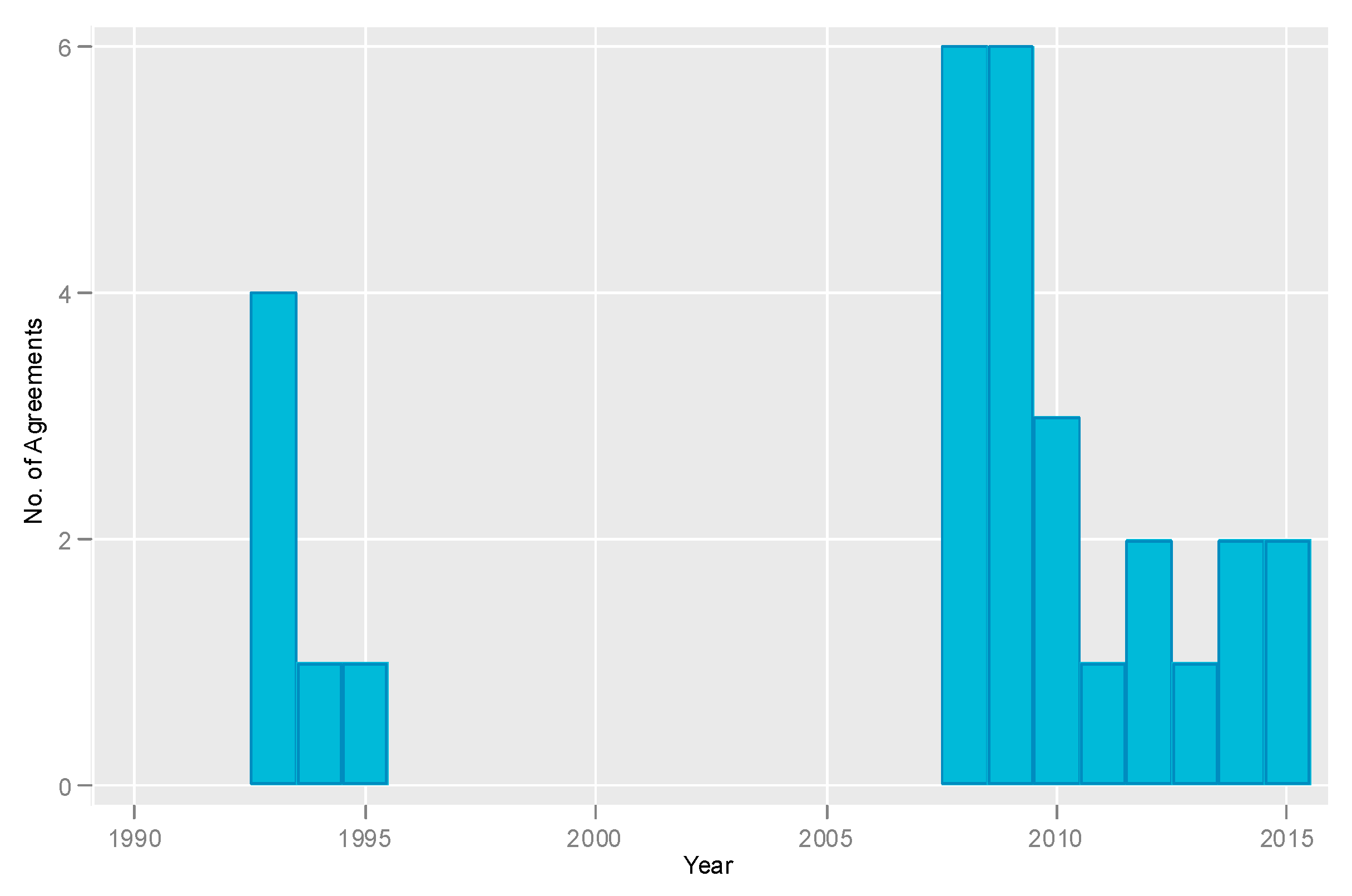
2.3. Contextualising Cross-Strait Relations

Taiwan and mainland China paused communication after the civil war in 1949. Taiwan was initially also an outcome of the Cold War. The Chinese Communist Party (CCP) established the People’s Republic of China (PRC) in Beijing, while Kuomingtang (KMT) moved the Republic of China (ROC) to Taiwan Island. It was only in the 1990s, when the two sides started to have some informal contact related to trade and investment, that communication was temporarily resumed. In Taiwan, the Straits Exchange Foundation (SEF) was established in 1991, which acted as an informal communication platform with the mainland. In the same year, the institution for dealing with Taiwanese affairs, the Association for Relations Across the Taiwan Straits (ARATS), was also founded in the mainland. These two institutions represent an important signal of the level of confrontation between Taiwan and the mainland. During the formal meetings at the 1992 Koo-Wang Summit through SEF and ARATS, both admitted that there was only one China in the world. The agreement of the One-China Principle is referred to as the 92 Consensus1 (Jiu er Gongshi, 九二共识). The 92 Consensus did not stipulate the exact meaning of “One China”, and both Taiwan and mainland China have their own interpretations. This ambiguity has also led to conflicts regarding differences in interpretation in different periods of time (Chu 1997; Bolt 2001; Yang and Hung 2003; Tsai 2017).

Two presidents of Taiwan, Lee Teng-hui (1988–2000) and Chen Shui-bian (2000–2008), held more conservative attitudes towards the One-China Principle (see more details of major political events 1991–2008 in Appendix D). Additionally, stalled formal talks between Taiwan and mainland China after 1995 added more turmoil to the political situation. In general, four main events worsened cross-strait relations and brought about regional political instability: the diplomatic visit to the United States in 1995, four military inspections across the Taiwan Strait, the proposition of the ‘two states theory’ in 1999, and the independent referendum in the early 2000s. These major events primarily show the constant tension from the 1990s to the middle of the 2000s (Cai 2011; Dittmer 2017). In general, the cross-strait relations between 1990 and 2008 have experienced great uncertainty with the cease of formal contact and periodic military threats.

In 2008, President Ma Ying-jeou (2008–2016) delivered his inauguration speech, stating that the 92 Consensus would be the basis for cooperation with the mainland, in the pursuit of reconciliation and truce (Zhang 2011). President Ma adopted the strategy of cooperating with the mainland and resumed all formal contacts with the mainland government, especially in the economic area. President Ma broke the political gridlock across the Taiwan Strait and resumed the dialogue between SEF and ARATS after a 13-year pause, which was the path to the normalisation of cross-strait relations (Tsai 2017). The normalisation of political relations between Taiwan and mainland China included several major events: the re-establishment of formal contact between SEF and ARATS; public recognition of the One-China Principle; and the establishment of the Three Links, where in the same year, direct trade, shipping transportation, and postal links were established, with these services being called the Three Links (san tong, 三通). Politically, both sides re-recognised the One-China Principle and resumed formal contact. Economically, both sides removed the previous limitations on investment and trade and established direct trade, postal, and transportation services. The previous political tension had suppressed the openness to investment and trading on both sides (Cheung 2007; Chiu 2016). Figure 2 and Figure 3 show the number of meetings and agreements signed regarding political and economic issues between Taiwan and the mainland during the period from 1990 to 2015. A dramatic increase in bilateral communication can be observed after 2008.

Responding to the policy–institutions framework, Ma Ying-jeou’s policies covered the principles of ‘promissory agreements’ and ‘soft balancing’ (Chen 2013, p. 31), which maintained Taiwan’s security and safety, while promoting liberal economic exchanges with the mainland. These strategies promoted official and informal bilateral communication through SEF, ARATS, ECFA and other semi-official institutions, which ultimately led to a much more open and peaceful trading and investment environment in 2008. This diplomatic truce provided great commercial opportunities and liberal capital flow across the Taiwan Strait. With the reduction in political conflict, both sides were more likely to witness higher levels of trade and investment openness. Interstate peace better serves the commercial interests of both sides (Chen 2013; Tsai 2017). Meanwhile, these actions and events, recognised as the normalisation of cross-strait relations, acted as a positive signal, affecting the trading and investment choices made by investors. Investors were more willing to expand their industries on both sides and allow more capital inflow and outflow on the basis of political peace across the Taiwan Strait. These positive political signals equated to a lower risk premium, promoting trade and investment confidence and, as a result, economic development (Tung and Chu 2015).

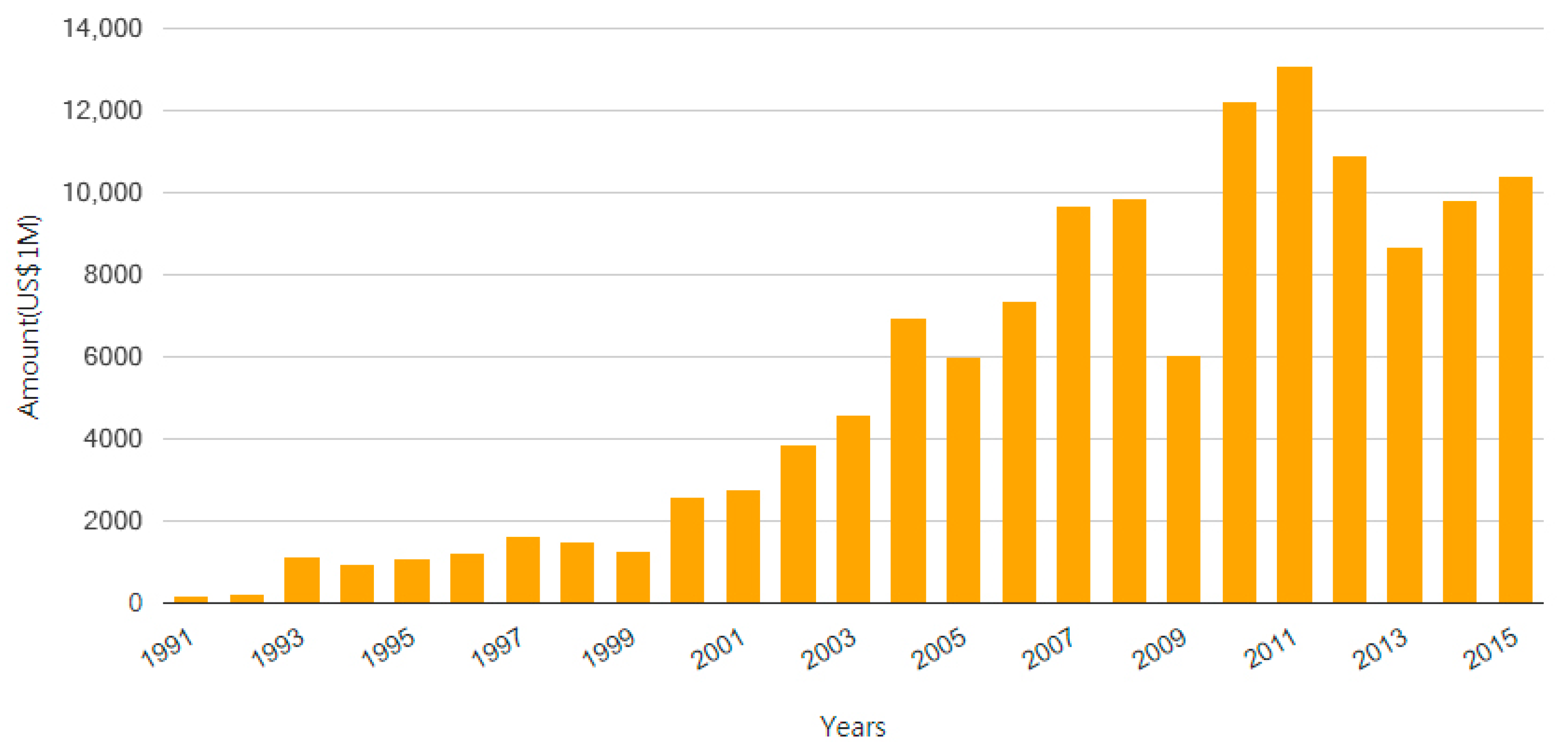
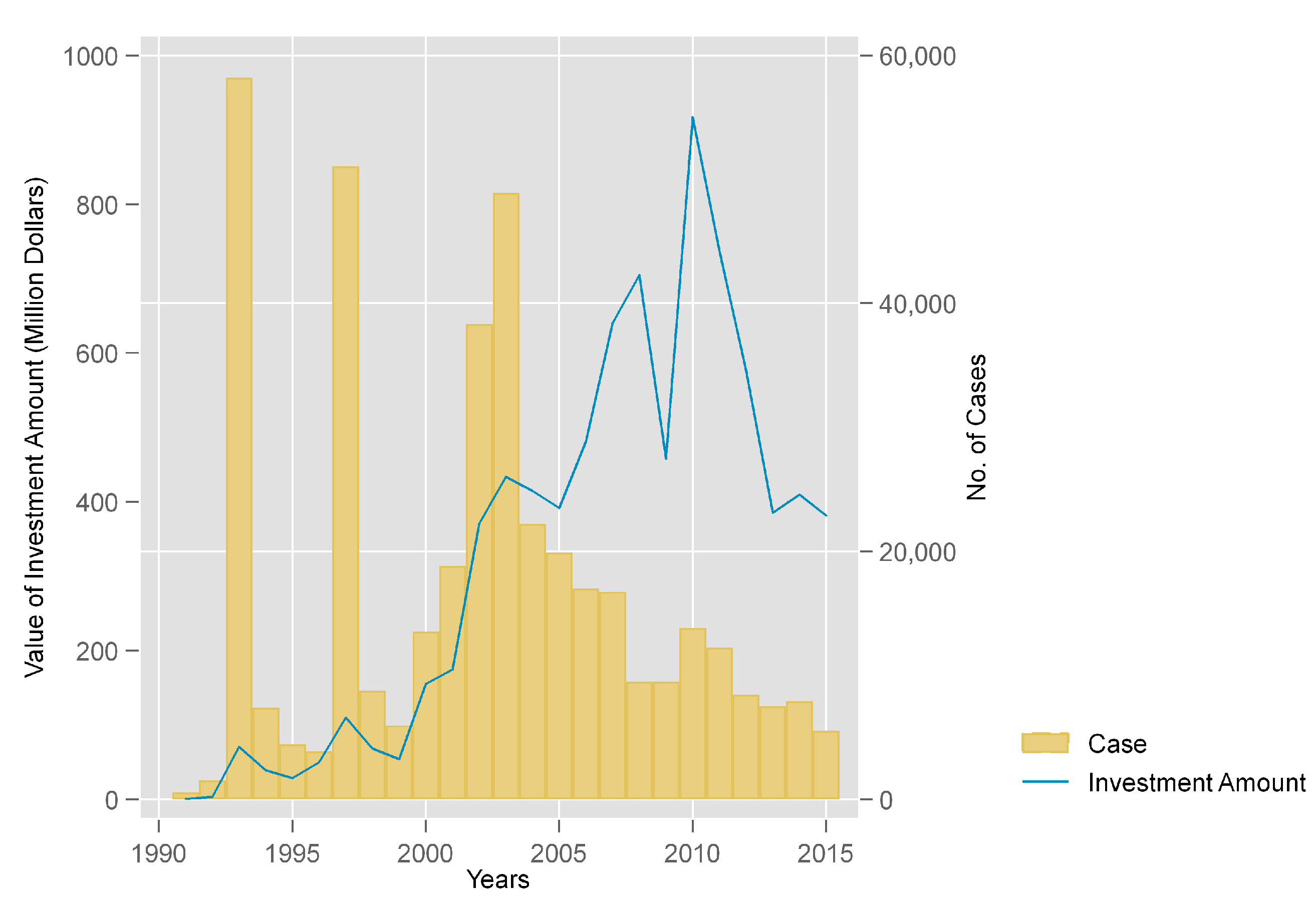
2.4. Economic Exchanges between Taiwan and Mainland China: Jiangsu Province as a Case Study

Geographic advantages, language similarity, and taxation benefits from the mainland resulted in greater business profitability in economic exchange between Taiwan and mainland China (Chase et al. 2004, also see Appendix B for Investment countries/regions of Taiwan (1991–2015)). Since the 1980s, Taiwan has faced increasing costs related to its labour force. Some Taiwanese industries moved to the mainland to maintain low production costs; thus, these products guaranteed their price competitiveness in the global market. For mainland China, the capital flow from Taiwan is the primary motivation and source of technology and industrial upgrades. Initially, Taiwan’s indirect investment was mainly focused on labour-intensive industries and agricultural projects. People in business transferred manufacturing and assembly operations to the mainland and then shipped these products to the global market, decreasing labour and land costs (Conable and Lampton 1993). In the early 1980s, the high-technology industries invested in Taiwan were concentrated in Guangdong province. In the 2000s, these technologies and high-profit productions were gradually transferred to the areas around the Yangtze River delta, especially Jiangsu province.

Jiangsu province has gradually become a closer partner for trade with Taiwan to accommodate the shifting investment priorities, which means that the economic development in Jiangsu province has had a more integrated relationship with direct investment from Taiwan (Figure 4). More specifically, Jiangsu province has gradually become the focus of direct investment from Taiwan since the 2000s. The economy of Jiangsu province is based on the manufacturing of high-tech and light electronic products, thus satisfying Taiwan’s shifting investment and production needs. The economic connection can be seen in the trajectories of investment changes in terms of both total investments from Taiwan and their allocation to Jiangsu province, which show a parallel trend (see Figure 5). A complete and stable production, sales and technology upgrade system has been built in the Yangtze River region. Jiangsu province has strong economic ties with Taiwan through trade and investment. Kunshan in Jiangsu province has become another ‘Silicon Valley’ for Taiwan’s information technology industries. Most high-tech and high-profit industries that have been invested in by Taiwan are based in Kunshan. Jiangsu province receives almost half of the direct investments from Taiwan and is gradually receiving core technology. The quality of cross-strait relations might significantly affect Chinese-based business from Taiwan. As a result, this would substantially influence Jiangsu’s GDP.

3. Data and Methods

Many scholars have been interested in measuring and evaluating the impact of specific policies on the basis of panel data that have been observed and collected over time, and in comparing the changes in some indicators before and after policy changes. However, most policy changes are not random, and the confoundedness from the observed covariates is potentially invalid and not credible (Abadie et al. 2015). Rigorous models are needed to address these issues, particularly the issue of unobserved counterfactuals. The difference-in-differences (DiD) model and synthetic control methods have been applied in different studies and empirical applications. DiD is recognised as appropriate for research in which the assumption of ‘parallel trends’ is made (Abadie 2005). That is, it is implied that the researcher is able to control for selection effects by considering fixed effects in time and units (Angrist and Pischke 2009). In comparison, synthetic control methods highlight the setting of a single or a certain group of exposed units, with the intent being to identify compensation for the missing parallel trends and re-weight all units to reveal the pre-exposure trends. Although these two methods have not often been applied together, and have been used differently, the assumptions of these two methods connect them together in this research.

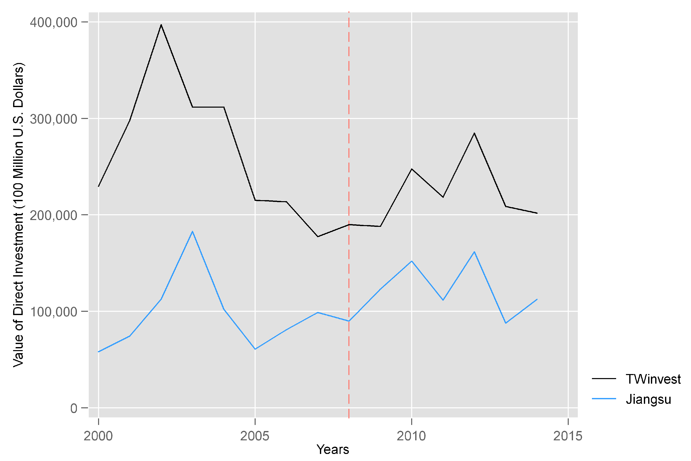
3.1. Data Source and Introduction

The government has divided mainland China into four regions: western, middle, northeast, and eastern China. The treated unit, Jiangsu province, is in eastern China. The rest remained untreated from 2008 to 2015. Secondary data were obtained from the public data available in the China Statistical Yearbook, the China Compendium of Statistics 1949–2008, the China External Economic Statistical Yearbook, and the Regional Statistical Yearbook. With open access, the data were retrieved from the official government websites, including the State Council, the Ministry of Civil Affairs, the Family Planning Commission and the Labour and Social Security Bureau. Here is an introduction of the important variables included in the models:

Dependent Variable: GDP per capita

Predictors: This research excludes Chongqing from the case study because Chongqing was still under the regulation of Sichuan province before 1997. The predictors include the percentage of total Investment in Fixed Assets on regional Gross Domestic Product (GDP), the percentage of primary industry (farming, farming, forest, agricultures) GDP of regional GDP, the percentage of industry GDP of regional GDP, the percentage of construction GDP of regional GDP, the percentage of transport, storage, and post GDP of regional GDP, the percentage of wholesale GDP of regional GDP, the population, the percentage of the population that is employed, and international export–import values. Due to the variations in size and unequal measurement values across these variables in different provinces, the percentage format is more accurate for the purpose of comparison. The author calculated these percentages based on raw data from the above-mentioned data sources.

Research Periods: All variables and predictors described above covered the period from 1990 to 2015. The pre-intervention period was from 1990 and 2008. The post-intervention period was from 2008 to 2015.

Treatment Exposure: This research focusses mainly on the impact of the normalisation of cross-strait relations since Ma Yin-jeou became the president of Taiwan in 2008. The commitment to the One-China Principle and the re-establishment of formal contact symbolises the normalisation of political relations between Taiwan and mainland China.

3.2. Research Modelling and Hypotheses

Hypothesis: The normalised cross-strait relations after 2008 positively and significantly increased economic growth (per capita GDP) in Jiangsu province. The basic model of the difference-in-differences method was used to test this hypothesis:

$${Per Capita GDP}_{it}={\delta }_{Jiangsu}+{\lambda }_t+{(\delta }_{Jiangsu}\times {\lambda }_t)+{\gamma }_r+{\mu }_t+{\epsilon }_{it}$$

(1)

${Per Capita GDP}_{it}$ is the outcome variable, being the per capita GDP of province i in the year t. ${\delta }_{Jiangsu}\times {\lambda }_t$ is the treatment effect of normalised cross-strait relations. This interaction term contains binary dummy variables, in which ${\delta }_{Jiangsu}$ is “1” for Jiangsu province and ${\lambda }_t$ is “1” for all provinces after 2008. ${\gamma }_r$ denotes the provincial fixed effects and ${\mu }_t$ denotes the year fixed effect. ${\epsilon }_{it}$ is the error term.

In the synthetic control method, the basic model for estimating the per capita GDP gap between Jiangsu province and its synthetic counterpart is as follows:

$$Y_{it}=Y_{it}^N+{\alpha }_{it}{D}_{it}$$

(2)

$Y_{it}^N$ is the per capita GDP of the synthetic unit in the absence of normalised cross-strait relations. $D_{it}$ is a dummy variable denoting the presence or absence of policy. ${\alpha }_{it}$ represents the estimate for the changes in per capita GDP. Detailed Stata command is attached in Appendix A for further information.

3.3. Synthetic Control Method

The political environment has a very important impact on economic development, yet quantitative analyses of this impact are lacking. One of the main reasons for this is that research on this issue is often “counterfactual”, making it difficult to measure the economic performance of an unstable economy in a favourable political environment, and thus to perform accurate quantitative analyses. The recent emergence of the synthetic control method in comparative case analysis offers a way of overcoming this difficulty (Abadie and Gardeazabal 2003; Abadie et al. 2015). In the synthetic control method, comparison units are used to reproduce the counterfactual of the treated unit in the absence of intervention. If we want to compare the units accurately, it is necessary to choose appropriate and suitable comparison units to articulate a precise counterfactual for the purpose of comparison. Comparison units are required to be similar enough to represent the case of interest in the pre-intervention period. Otherwise, the gap between the intervention units and the comparison units may be a result of their systematic differences rather than the impact of the treatment. Additionally, the mechanisms by which comparison units can be chosen are full of complications. The synthetic control method specifies the ways in which different comparison units can be chosen from the donor pool.

This method suggests that an aggregate of entities is better abel to reproduce the features of the unit of interest than a single comparison unit. Countries, states, or regions are aggregated entities that can be used for better comparison (Lijphart 1971; George and Bennett 2004). The comparison units reproduce the features of the intervention units in the form of a weighted average, and are used to synthesise a synthetic unit in the absence of intervention. The synthetic control method defines how each comparison unit is weighted to construct a proper counterfactual (Abadie et al. 2015). The explicit proportion of each comparison unit illustrates the different characteristics of the comparison units and their relationship to the unit of interest. Only certain provinces can be used to represent economic development similar to that of Jiangsu province before the changes in cross-strait relations. A weighted average constructed from the provinces with similar characteristics provides an appropriate and similarly matched stimulation of Jiangsu province in the pre-intervention period from 1990 to 2008. The synthetic control method can ultimately generate a counterfactual that acts as the economic trajectory of the treated unit in the absence of the normalisation of cross-strait relations in 2008.

Technically, there are J + 1 units (e.g., provinces) coded by j. j = 1 means the unit of interest, while the rest, e.g., j = 2, j = 3, are the comparison units. Unit j = 1 is the unit exposed to the intervention, and the comparison units, j = 2 to j = J + 1, construct a ‘donor pool’. The comparison units in the donor pool are used to estimate the outcomes for the synthetic unit of interest, j = 1, under a situation without any intervention.

Jiangsu province is the unit of interest, and the donor pool includes 29 provinces and municipalities. The sample is a longitudinal dataset, among which all units are observed and recorded in the same periods, from $t=1$ to $t=T$. The data set includes several pre-intervention periods, from $t=1$ to $t=T_0$. The unit $j=1$ receives the intervention during the period from $t=T_0+1$ to $t=T$. The intervention does not have any impact during the period from t = 1 to t = $T_0$. In this research, the effect of the intervention is estimated by comparing the results obtained during the post-intervention period between the synthetic GDP per capita and the actual GDP per capita GDP. Compared to a single comparison unit, the combination of comparison units can be much more precise in estimating the characteristics of the treated unit before intervention (Lijphart 1971; Abadie et al. 2015).

$Y_{jt}$ is the outcome of the unit j in the period t. $Y_1$ is the $\left(T_1\times 1\right)$ vector that collects the outcome of the treated unit during the post-intervention period (Abadie et al. 2010). Therefore, $Y_1={(Y_{1T_o+1},\dots ,Y_{1T})}^{\prime }$. For the outcome of the comparison units, $Y_0$ is the $\left(T_1\times J\right)$ matrix, in which J includes the outcome values for the unit $=j+1$. The estimate of the impact of the intervention is estimated by comparing the results of the treated unit and the outcomes from the synthetic control during the post-intervention periods ($t\ge T_0)$.

$$Y_{1t}-\sum _{j=2}^{J+1}{w}_j^{\mathrm{*}}{Y}_{jt}$$

(Abadie et al. 2015, p. 498)

Only nearly identical units in both the observed and unobserved predictors can produce similar trajectories in outcome estimators before the intervention, resulting in the construction of better counterfactual and comparison units (Abadie et al. 2015). Moreover, once such a synthetic control unit has been constructed, it can be used to represent treated units that share similar dynamics before the intervention. Thus, the discrepancy in outcome variables after the intervention corresponds precisely to the impact of the intervention.

The synthetic per capita GDP of Jiangsu province can be constructed as a weighted average from the control provinces, showing the per capita GDP of Jiangsu province if it were not influenced by the changes in cross-strait relations. The gap between the synthetic per capita GDP in Jiangsu province and the actual per capita GDP in Jiangsu province is exactly the causal effect of the changes in cross-strait relations. By synthesising the comparison units, this approach provides a better counterfactual for the intervention units and overcomes the disadvantages of traditional regression methods (Abadie et al. 2010).

To complement the synthetic control method, a reducing comparison unit test was also conducted in this research, and a pattern similar to that found by Abadie et al. (2015) was observed: the use of fewer comparison cases led to greater bias and uncertainty. Increasing the number of comparison units in the comparison groups can reduce estimating bias, generating a more credible comparison counterfactual. The selection of comparison units for this method provided a more accurate and robust result with respect to causal inference.

3.4. Difference-in-Differences (DiD)

Under the assumption that the constant changes between the treated units and the comparison units across time, the difference-in-differences (DiD) method compares the outcome variables of both the treatment and the comparison groups in the pre-intervention and post-intervention periods. Furthermore, DiD assumes that any time effects (e.g., exogenous shocks) will have the same influence on both the treated and comparison units in the pre-intervention period. These two assumptions are denoted the ‘parallel trend assumption’. If there are no interventions between these units, the treated and comparison units will have parallel trajectories over time. The gap in the outcome variables between the treated units and the comparison units will be the same in the absence of treatment (Angrist and Pischke 2009; O’Neill et al. 2016). However, if the treated units receive treatment, the gap between the units of interest and other comparison units will undergo changes. That is, if treatment has an impact following the intervention, the trajectories of the outcome variables will no longer be parallel. Whether this assumption is guaranteed is the key to the credibility of the difference-in-differences estimation (Ryan et al. 2015).

In the difference-in-differences design, the average effect of normalised cross-strait relations is the difference between the observed outcome after 2008 and the counterfactual outcome produced based on parallel trend assumptions. The causal effect is called the average treatment effect for the treated (ATT).

$$\mathrm{D}\mathrm{i}\mathrm{f}\mathrm{f}\mathrm{e}\mathrm{r}\mathrm{e}\mathrm{n}\mathrm{c}\mathrm{e}-\mathrm{i}\mathrm{n}-\mathrm{d}\mathrm{i}\mathrm{f}\mathrm{f}\mathrm{e}\mathrm{r}\mathrm{e}\mathrm{n}\mathrm{c}\mathrm{e}\mathrm{s} \mathrm{e}\mathrm{s}\mathrm{t}\mathrm{i}\mathrm{m}\mathrm{a}\mathrm{t}\mathrm{i}\mathrm{o}\mathrm{n}=\left({\overline{Y}}_{Treated}^{After}-{\overline{Y}}_{Treated}^{Before}\right)-\left(Y_{Comparison}^{After}-Y_{Comparison}^{Before}\right)$$

(Imai 2017, p. 62)

${\overline{Y}}_{Treated}^{After}-{\overline{Y}}_{Treated}^{Before}$ denotes the difference between the treated units after exposure to the treatment. $Y_{Comparison}^{After}-Y_{Comparison}^{Before}$ denotes the difference between the comparison units after the implementation of the policy. In a difference-in-differences design, the outcomes for the treatment units and the comparison units will exhibit parallel changing trends over time. The difference in the outcome variables in the treatment units before and after the implementation of the policy should be the same as the difference in the outcome variables in the comparison units before and after the treatment.

In observational studies, it is assumed that, in addition to treatment, the treatment and control units should be comparable in every covariate related to the outcome (Imai 2017). The pre-treatment variables related to the treatment and outcome variables are confounders. These confounders are a possible cause of confounding bias in outcome estimation. The existence of these variables can confound the causal effect, violating the validity of causal inferences, and making it difficult to examine whether the treatment or the confounders caused the observed outcomes. Counterfactual results for the treated units are measured under the assumption that the time trend for treatment units is parallel to that for the control units. The counterfactual outcome is the GDP gap per capita between Jiangsu province and the rest of the comparison provinces in the absence of normalised cross-strait relations.

If the estimation is greater/smaller than the before-and-after estimation, it means that the treatment has a negative/positive influence on the treated units (Imai 2017). If the counterfactual outcomes for treated units fail to parallel the trend of the comparison units over time, the credibility of the causal inferences in the difference-in-differences design will be violated. Thus, it is important to test this assumption by collecting adequate data in the pre-treatment period. Jiangsu province is not the only province to receive direct investment from Taiwan. Therefore, difference-in-differences could help to exclude other time-variant differences, including the effect of investment on other provinces. By using other provinces as comparison groups, differences-in-differences is able to distinguish the per capita GDP changes between Jiangsu province and the rest. The changes in the gap are the exact influence of the normalisation of cross-strait relations after 2008.

Difference-in-differences is creditable if the parallel-trend assumption is valid and unquestionable. In this case, Jiangsu province is compared with the remaining provinces, which did not receive or received little treatment with respect to normalised cross-strait relations. Therefore, the differences between the GDP before the intervention per capita and the GDP after the intervention per capita in Jiangsu province is not able to provide credible evidence of the economic impact of normalised political relations. Therefore, if the per capita GDP gap between Jiangsu province and the rest of the provinces in China is constant, this design can generate a credible counterfactual for the changes in per capita GDP in Jiangsu province. The counterfactual is that if Jiangsu province had not received any treatment for normalised cross-strait relations, it would have followed the same trend, maintaining a constant gap with the rest of the provinces. From Figure 6 and Figure 7, this parallel trend is initially valid in the model estimating the parallel trend with control variables.

4. Results

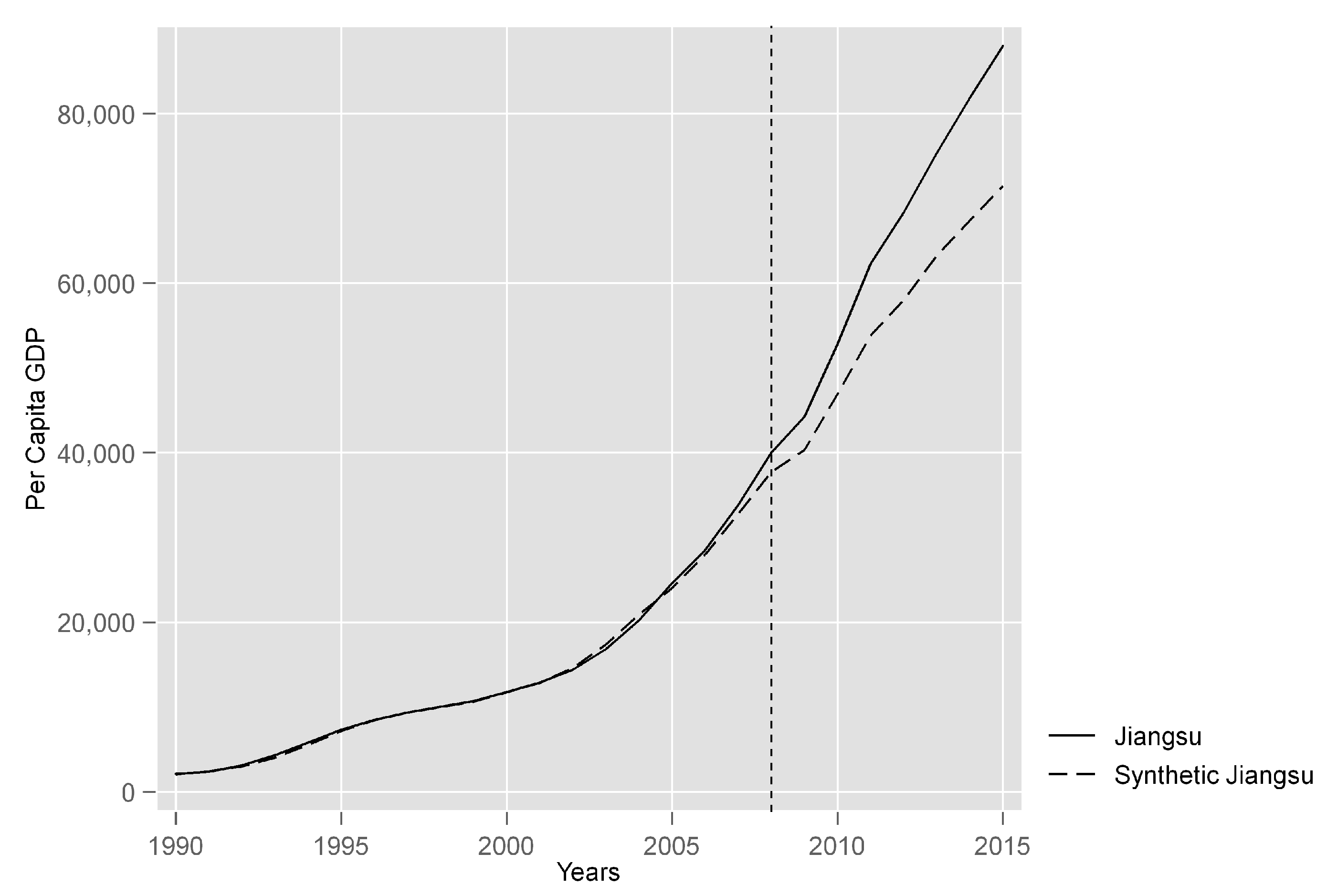
4.1. Results of the Design of Synthetic Control Methods

The trends of GDP per capita in Jiangsu province and the average GDP per capita in the rest of the provinces are plotted in Figure 8. The average per capita GDP of the other provinces cannot provide a proper comparison for Jiangsu province because the gap between them is not constant, and they were different before the normalisation of cross-strait relations. Although there was an obvious divergence in per capita GDP between all other provinces and Jiangsu around the end of the 2000s, it cannot be inferred that these changes were due to the normalisation of political relations between Taiwan and mainland China.

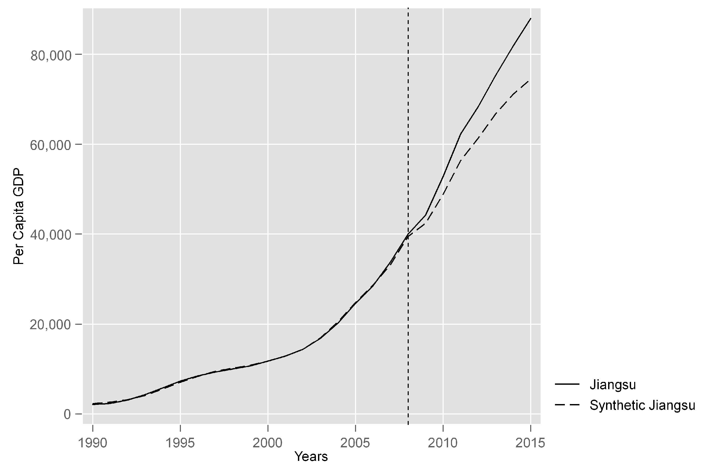
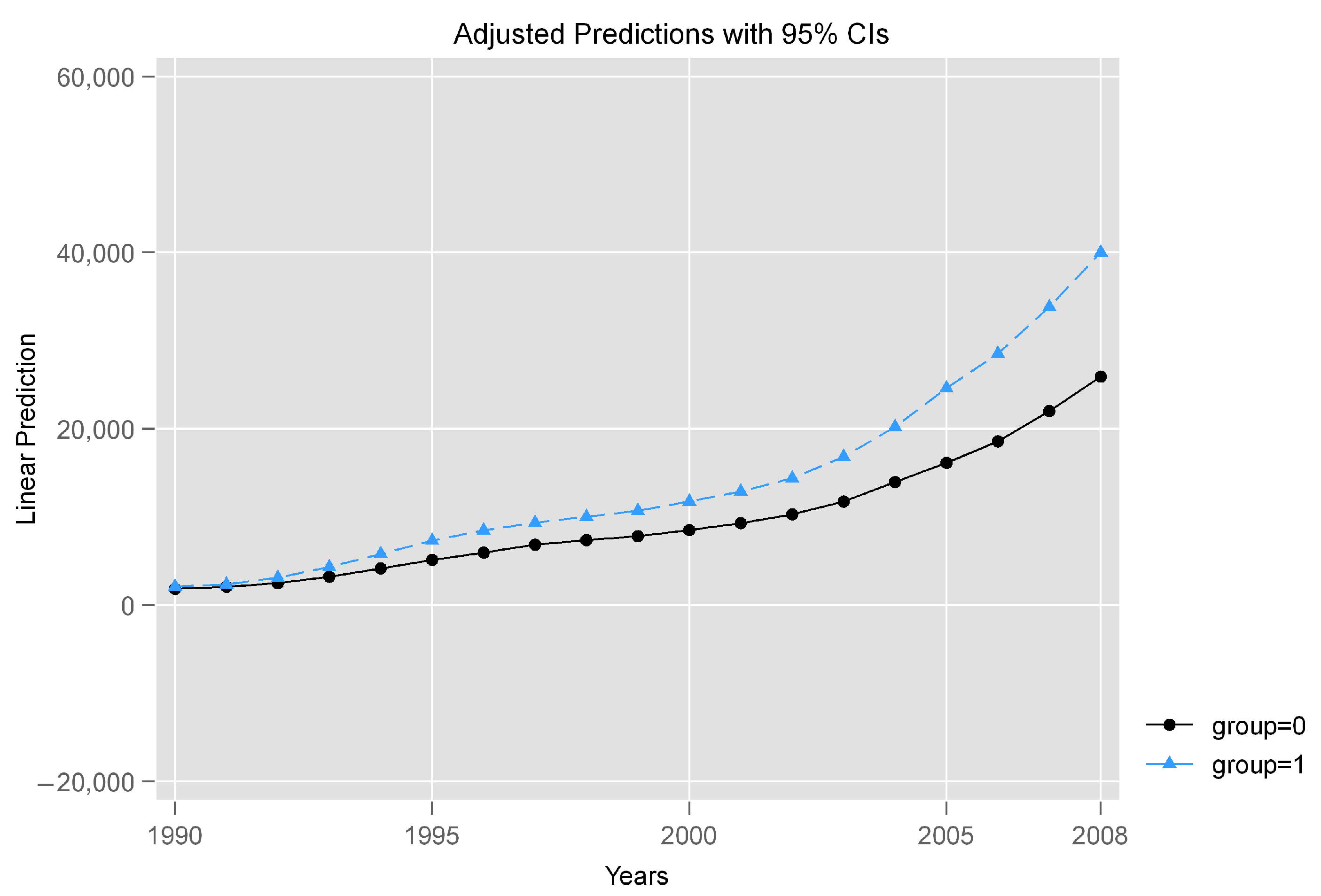
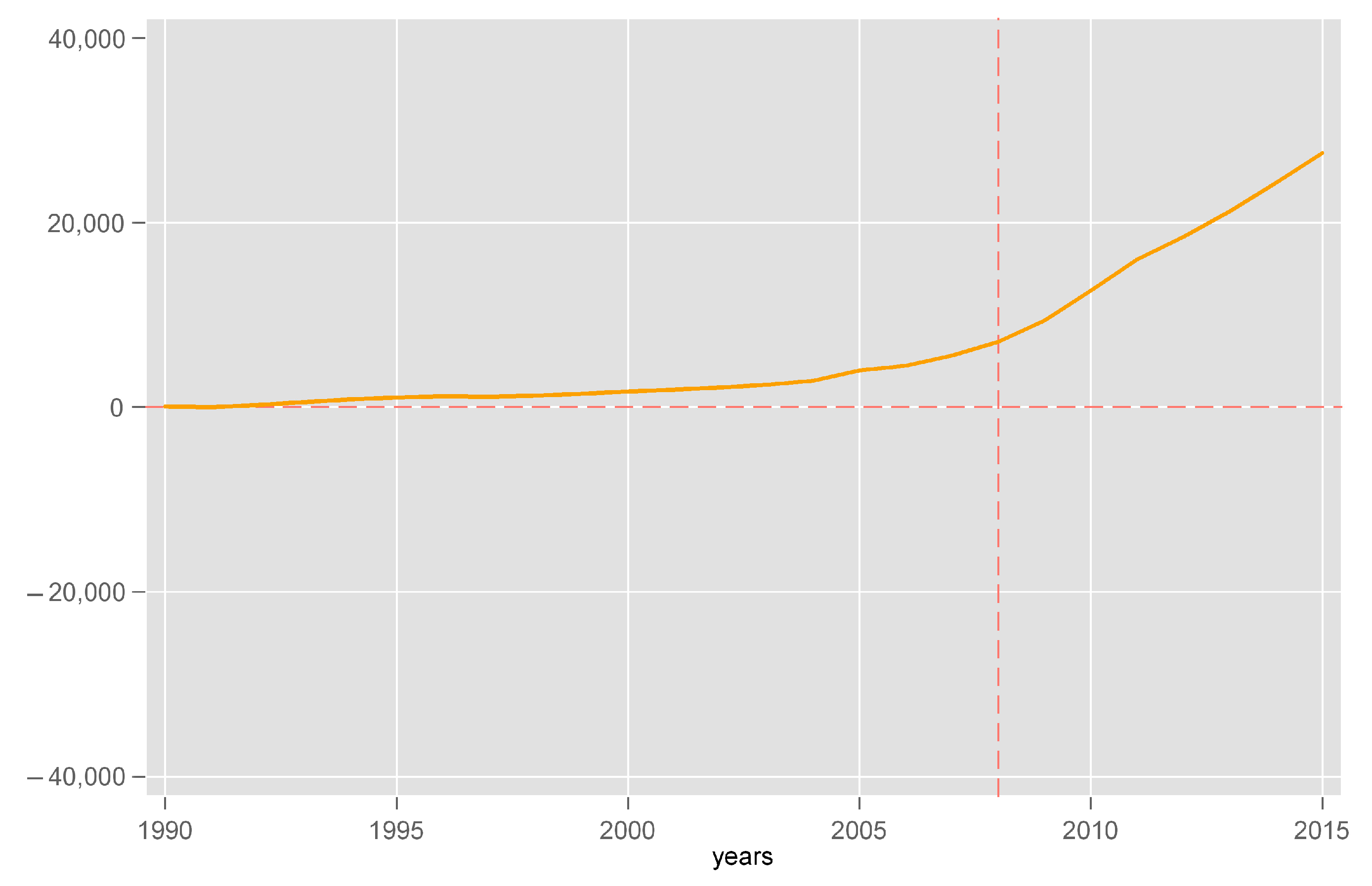
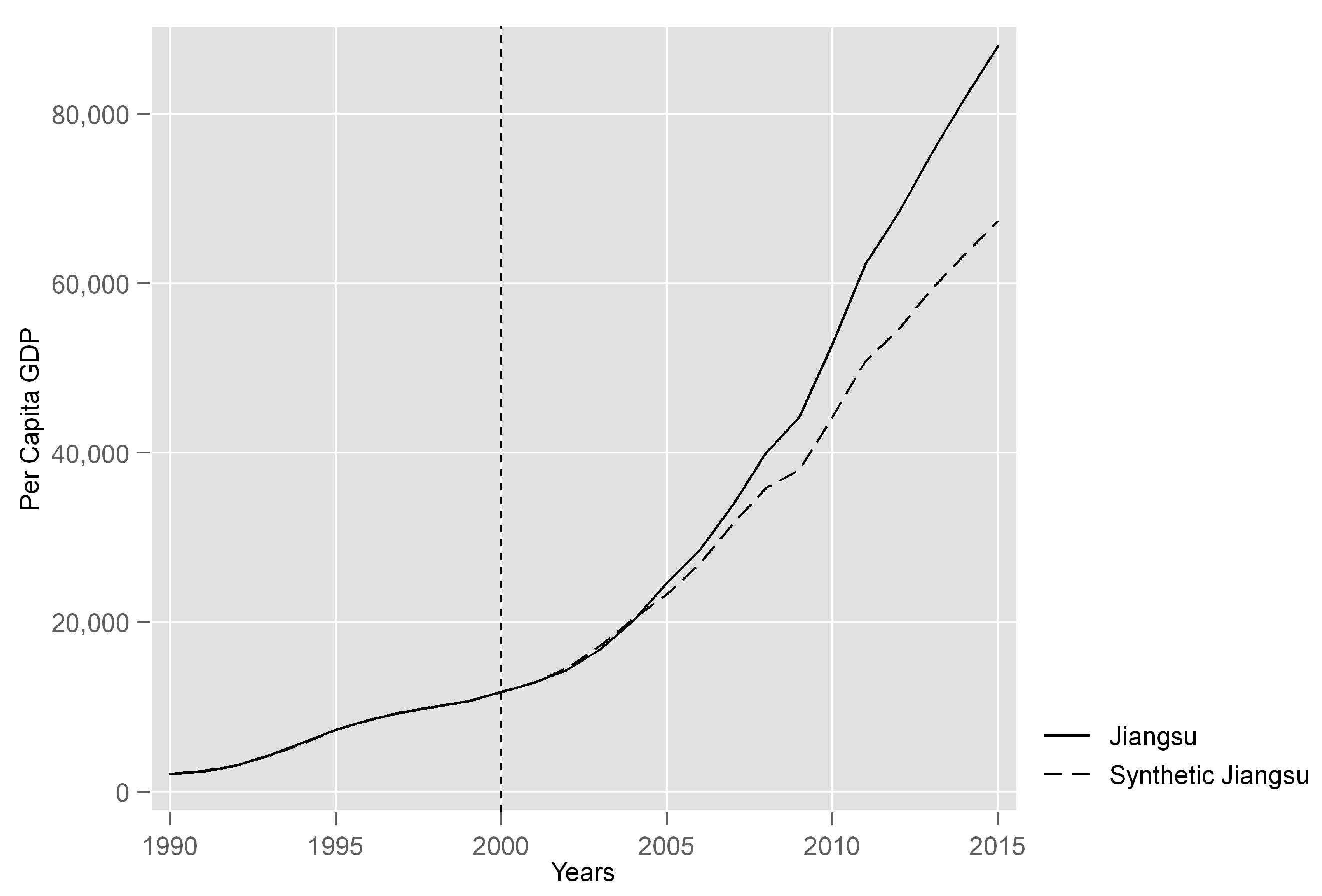
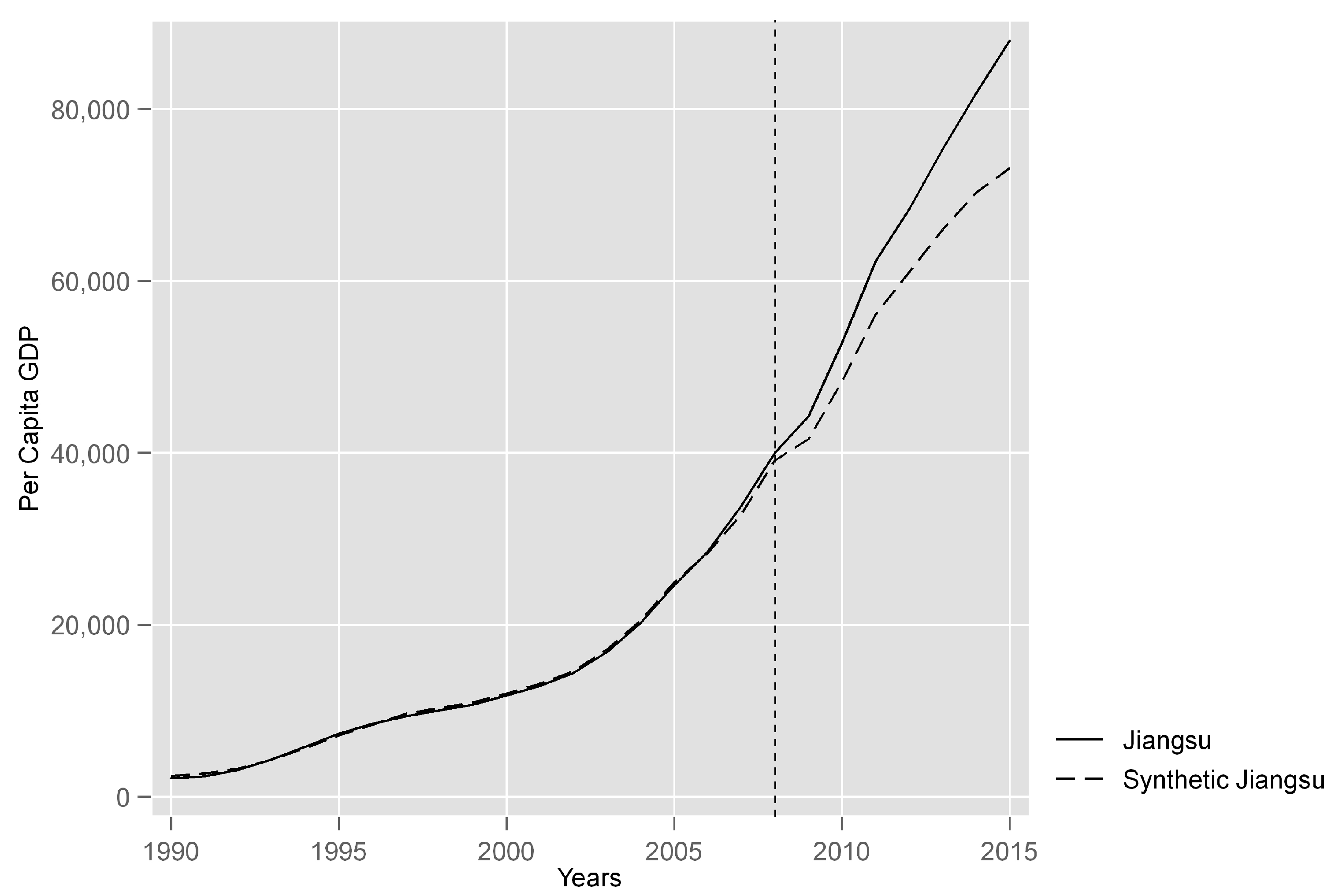
4.1.1. Baseline Result

The synthetic control method precisely generates the counterfactual in order to perform causal inference. As can be seen from both Figure 9 and

Table 1. Predictors of Jiangsu province and synthetic Jiangsu province.

	Jiangsu	Synthetic Jiangsu	Average of Comparison Provinces
PercentPrimary	0.205	0.207	0.279
PercentIndustry	0.466	0.458	0.371
PercentConstruction	0.057	0.053	0.068
PercentTranStoPos	0.049	0.063	0.065
PercentInvest	0.433	0.427	0.492
PerecentWholesale	0.099	0.107	0.094
PercentEmploymentPopu	0.609	0.581	0.530
ExpoImport	2082.027	1377.619	440.695
ln_Population	8.913	8.631	7.998

, the synthetic Jiangsu province nearly reproduces the exact per capita GDP of Jiangsu province in the pre-intervention period. The close-fit GDP predictors also reproduce economic characteristics similar to those of the actual Jiangsu province before the intervention. Given

Table 2. Synthetic weights of Jiangsu province.

Province	Synthetic Control Weights	Province	Synthetic Control Weights
Beijing	0	Henan	0
Tianjin	0.208	Hubei	0
Hebei	0	Hunan	0
Shananxi	0	Guangdong	0.167
Inner Mongolia	0	Guangxi	0
Liaoning	0	Hainan	0
Jilin	0	Sichuan	0
Heilongjiang	0	Guizhou	0
Shanghai	0	Yunnan	0
Zhejiang	0.05	Xizang	0
Anhui	0	Shanxi	0
Fujian	0	Gansu	0
Jiangxi	0	Qinghai	0
Shandong	0.575	Ningxia	0
		Xinjiang	0

, Shandong occupies the highest weight, 0.575, and the second is Tianjin, 0.208. Guangdong has a weight of 0.167 and Zhejiang 0.05. The rest of the provinces weigh 0. This means that the per capita GDP of Jiangsu province can largely be synthesised appropriately by Shandong and Tianjin. Namely, the synthetic counterpart can create a credible counterfactual of Jiangsu without treatment.

The causal effect is estimated by the difference in GDP per capita between the actual Jiangsu province and its synthetic counterpart. This effect is visualised in Figure 10. After 2008, the per capita GDP of Jiangsu province witnessed faster growth. It reports that the per capita GDP trajectories diverge substantially after 2008. Per capita GDP growth accelerated in actual Jiangsu from 2008 onwards, while that of its synthetic counterpart maintained a similar speed to that in the pre-intervention period. Per capita GDP in Jiangsu province increased by approximately CNY 2500 (about GBP 278) every year on average after 2008, which represents a nearly 6.5% increase per year from 2008 onwards. At the end of the research period, per capita GDP in actual Jiangsu province was approximately 19% higher than that of its synthetic counterpart. This empirical evidence illustrates that increased political stability between Taiwan and mainland China could bring about regional economic development and accelerate economic growth.

4.1.2. Spillover Effect: Other Specifications

One of the concerns in this study is the possible spillover effect. The normalisation of cross-strait relations influenced trading and investment across mainland China, even though many provinces did not have any economic exchange with Taiwan. Normalised political relations can also positively affect GDP per capita GDP in other provinces. For example, good political relations across the Taiwan Strait have a positive spillover effect on other provinces, and these were included in the donor pool. In such cases, the per capita GDP of the synthetic counterpart will overestimate the counterfactual in the absence of normalised cross-strait relations. Guangdong province, Shanghai, Fujian province and Zhejiang province receive a certain level of investment from Taiwan. Thus, they have a higher possibility of being influenced by the treatment, possibly undermining the estimates’ accuracy. Therefore, in this section, a spillover test is conducted to exclude those provinces with a higher possibility of experiencing spillover effects from the donor pool. The specification of excluding provinces with possible spillover effects from the donor pool will not affect the estimates (Abadie et al. 2015). This specification results in the data of Guangdong, Shanghai, Fujian province and Zhejiang province being dropped. Figure 11 and

Table 3. Predictors of Jiangsu province and synthetic Jiangsu province (spillover test).

	Jiangsu	Synthetic Jiangsu
PercentPrimary	0.205	0.221
PercentIndustry	0.466	0.443
PercentConstruction	0.057	0.055
PercentTranStoPos	0.049	0.061
PercentInvest	0.433	0.439
PerecentWholesale	0.099	0.106
PercentEmploymentPopu	0.609	0.591
ExpoImport	2082.027	887.309
ln_Population	8.913	8.651

report the results of implementing this specification. With a good fit between actual Jiangsu and synthetic Jiangsu, this specification model still shows a similar per capita GDP gap result in the baseline result. This test demonstrates the accurate and valid results analysed in the baseline model.

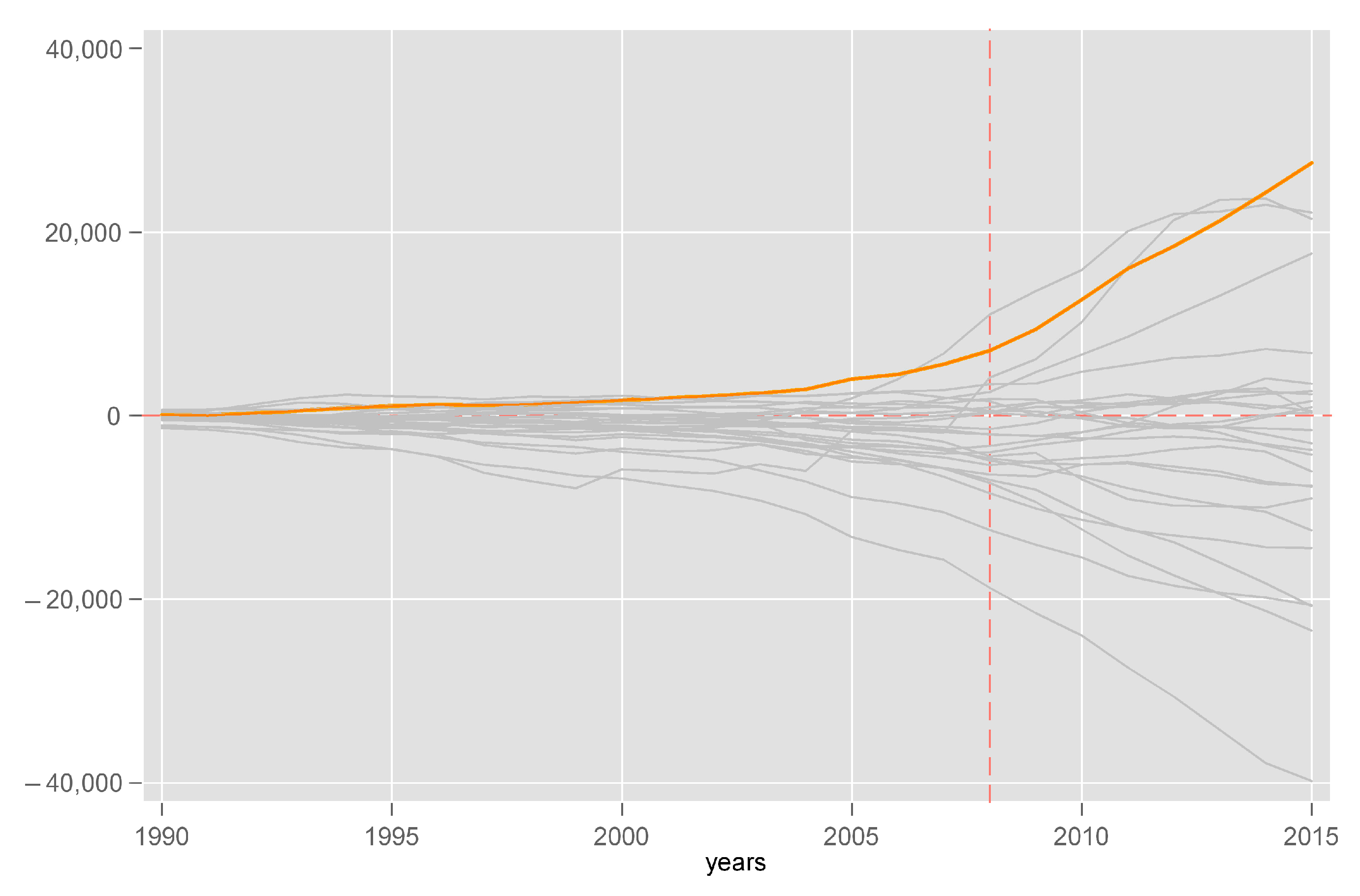
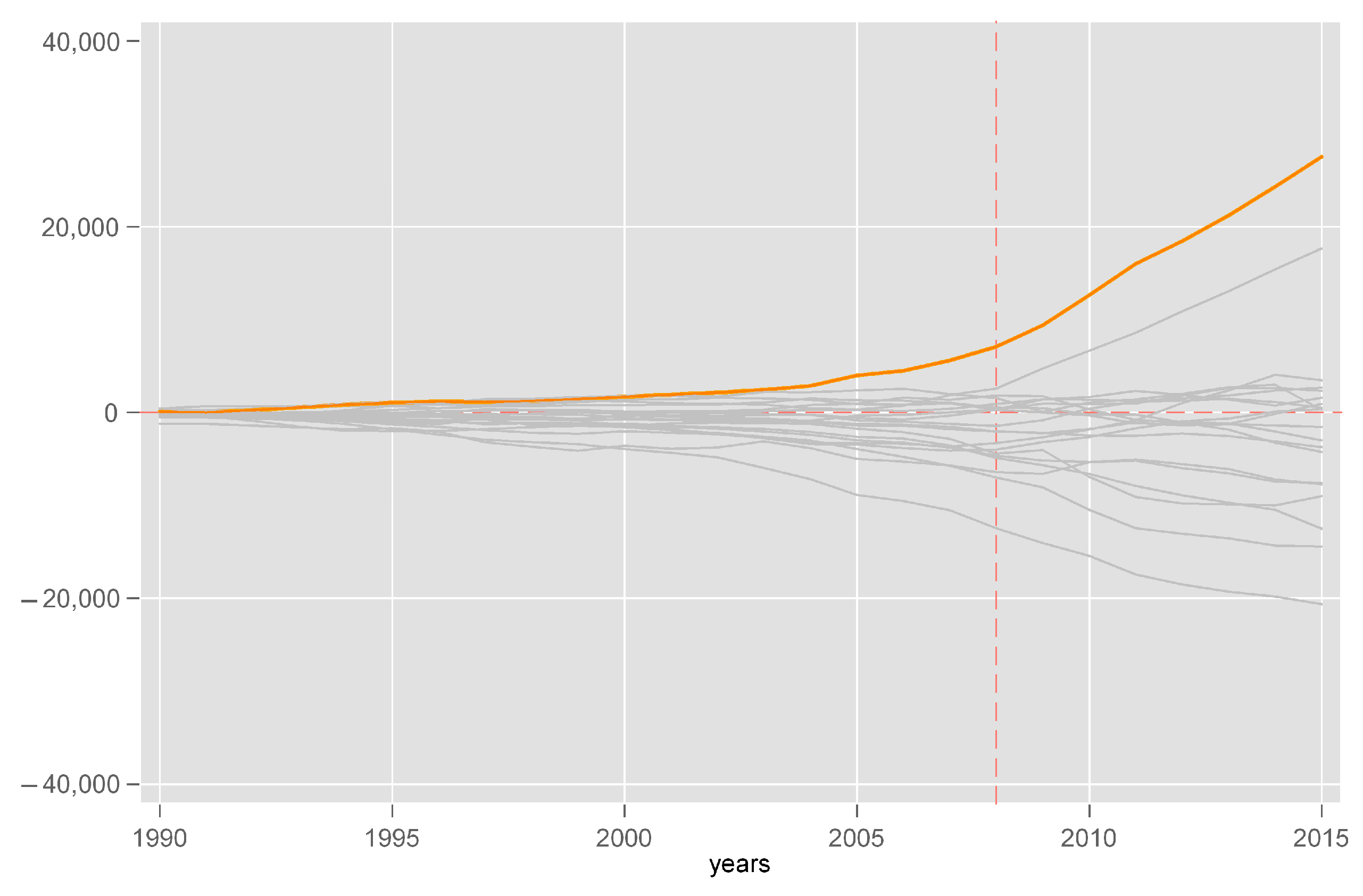
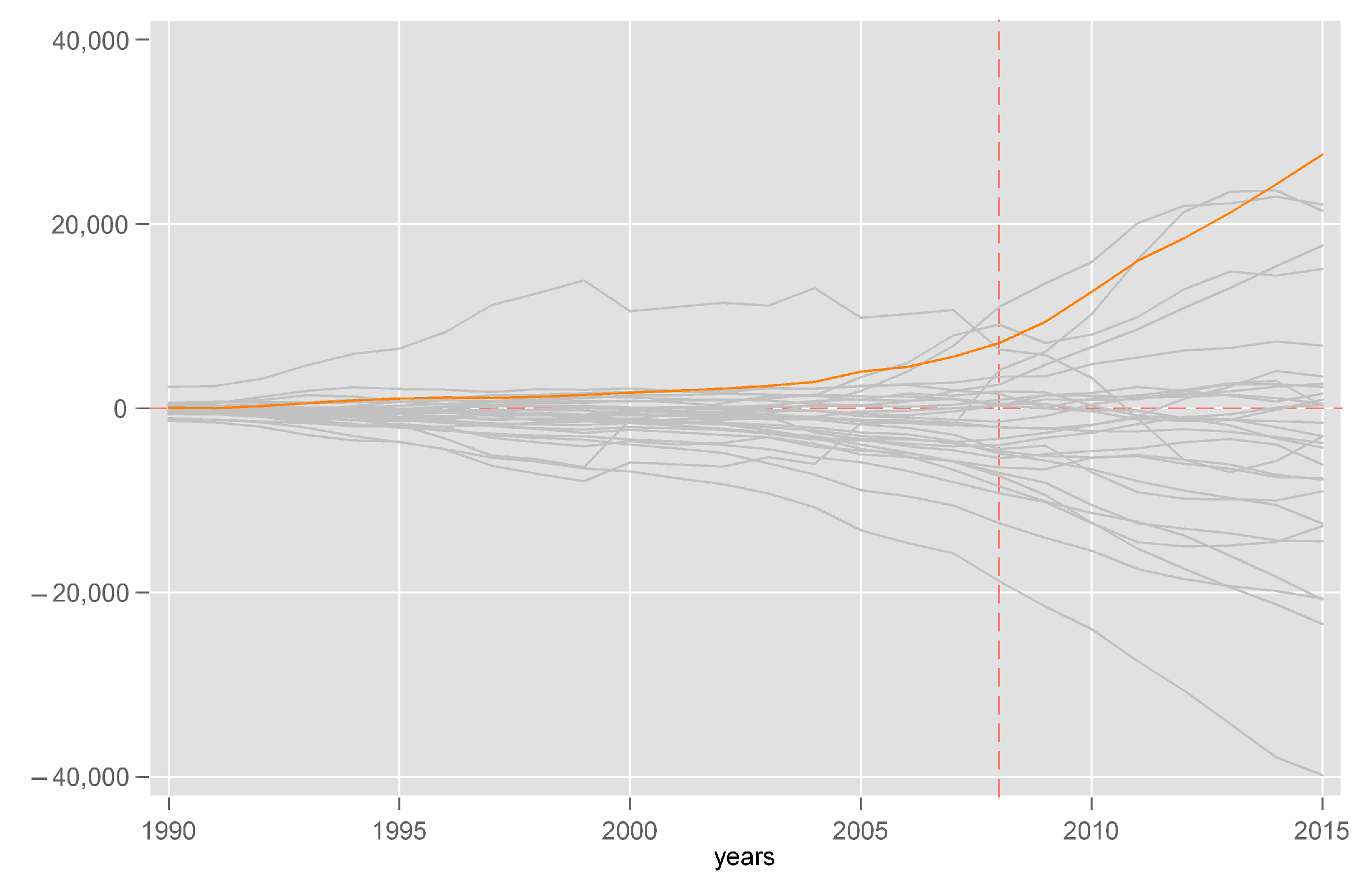
4.1.3. Placebo Test 1: Reassignment of the Treatment

Placebo tests and robustness tests are needed to test the sensitivity and robustness of the above results. This placebo test reassigns the treatment to the comparison provinces. The results present the effect of the treatment in each province and compare these estimates with the effect of normalised cross-strait relations in Jiangsu province. The estimated effect in Jiangsu province should be comparatively more significant than in the comparison provinces.

Figure 12 reports the estimated results of the placebo test. The grey lines show the gap in GDP per capita between the 29 comparison provinces and their synthetic counterparts when treatment was assigned to them. The orange line indicates the estimates for Jiangsu province. The estimated gap in Jiangsu province from 2008 to 2015 is significantly larger than the distribution of the gaps in the rest of the provinces within the comparison group. Therefore, the increase in GDP per capita in Jiangsu province is statistically significant at a level of 1/30, 0.033.

However, some provinces are not well reproduced. Placebo tests with a poor match in the pre-intervention period will not be able to provide accurate information for estimating the distribution (Abadie and Gardeazabal 2003; Abadie et al. 2010). Therefore, in the following results, some provinces with RMSPE values beyond a certain level prior to treatment will be excluded. Figure 13 excludes the provinces with pre-intervention RMSPE values more than ten times that of Jiangsu province. There are 27 provinces left in this figure. In this figure, the grey lines show the gap in GDP per capita between these 27 comparison provinces and their synthetic counterparts when treatment was assigned to them. The orange line while indicates the estimates for Jiangsu province. Figure 14 excludes the provinces that had RMSPE values more than five times that of Jiangsu province. There are 24 provinces left in this figure. In this figure, the grey lines show the gap in GDP per capita between these 24 comparison provinces and their synthetic counterparts when treatment was assigned to them. The orange line while indicates the estimates for Jiangsu province. The Jiangsu province gap line is much clearer, and is significantly higher than the rest of the comparison provinces.

Figure 13. GDP gaps per capita in Jiangsu (orange line) and placebo gaps in 27 provinces (grey lines, excluding provinces with pre-proposition 99 RMSPE ten times higher than Jiangsu’s)2.

Figure 13. GDP gaps per capita in Jiangsu (orange line) and placebo gaps in 27 provinces (grey lines, excluding provinces with pre-proposition 99 RMSPE ten times higher than Jiangsu’s)2.

Figure 14. GDP gaps per capita in Jiangsu (orange line) and placebo gaps in 24 provinces (grey lines, excludes provinces with pre-proposition 99 RMSPE five times higher than Jiangsu’s)3.

Figure 14. GDP gaps per capita in Jiangsu (orange line) and placebo gaps in 24 provinces (grey lines, excludes provinces with pre-proposition 99 RMSPE five times higher than Jiangsu’s)3.

To get a better version of the estimates that have been further well-fitted in the pre-intervention period. Figure 15 excludes the provinces with a pre-intervention RMSPE more than twice the Jiangsu province. There are 21 provinces, highlighted in grey colour, left in this figure. The Jiangsu province, shown through the orange line, is the highest of all. Therefore, if you randomly pick a province, the possibility of getting a gap of this magnitude is 1/21, approximately 5%, which is statistically significant. In this figure, the most properly matched units are shown. Jiangsu province is still the most significant province with an obvious increase in GDP per capita compared with the synthetic unit.

Figure 15. Per capita GDP gaps in Jiangsu (orange line) and Placebo Gaps in 15 provinces (grey lines, excludes provinces with pre-intervention RMSPE twice as high as Jiangsu’s)4.

Figure 15. Per capita GDP gaps in Jiangsu (orange line) and Placebo Gaps in 15 provinces (grey lines, excludes provinces with pre-intervention RMSPE twice as high as Jiangsu’s)4.

At the end of this placebo test, the figures show the ratio of RMSPE before 2008 and the RMSPE after 2008. The value of RMSPE represents the degree of proper matching before 2008. If the value of RMSPE before 2008 is low, then it means that the synthetic unit is properly matched to the actual conditions. Supposing that the normalisation of political relations after 2008 was influential, and the per capita GDP of Jiangsu province was greatly affected by this treatment, in this case, the RMSPE ratio after 2008 and the RMSPE before 2008 should be larger than those of the other provinces.

The ratios of post-intervention to pre-intervention RMSPE are shown in Figure 16. The ratio for Jiangsu province, highlighted in red, is 11.0737, which higher than the rest of the other provinces. If randomly picking a province, the possibility of receiving a ratio as high as the unit of interest would be 1/30, or about 0.033; by measuring the ratio, mistakes in the estimates can be avoided due to the unfitted placebo distributions in the previous figures (Abadie et al. 2010). According to this placebo test, compared to the initial economic development under confrontational political relations, normalised political relations between Taiwan and mainland China could increase the per capita GDP in Jiangsu province, a region with close economic ties with Taiwan.

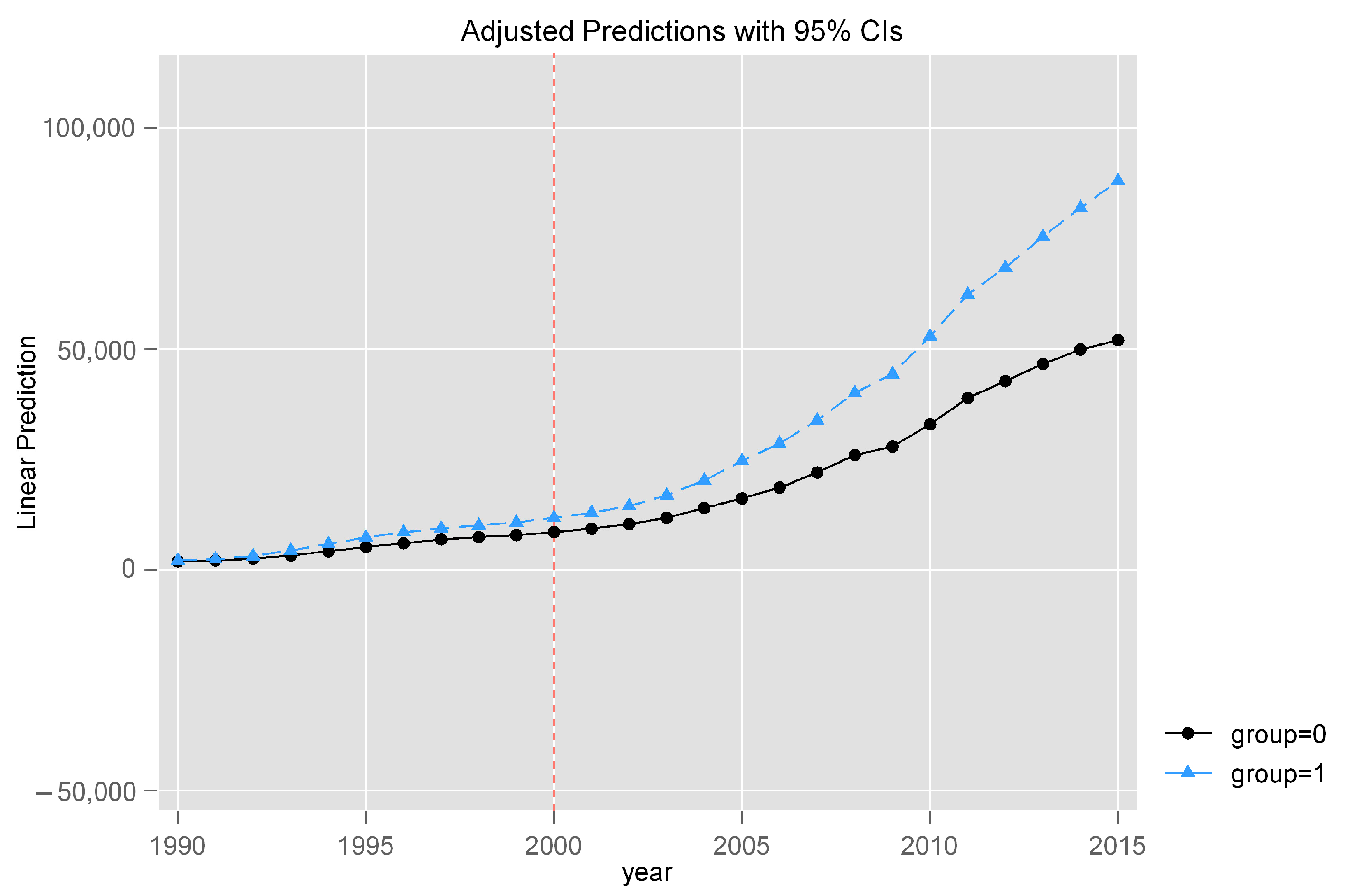
4.1.4. Placebo Test 2: Normalisation of Cross-Strait Relations in 2000

In the second placebo study, the treatment was reassigned to the year 2000, eight years earlier than the actual normalisation of political relations. Other than the time, the rest of the technique is the same as for the baseline model. According to Figure 17, the per capita GDP of Jiangsu and synthetic Jiangsu did not diverge obviously from 2000 to 2008. Namely, this placebo test in which the normalisation of political relations occurred in 2000 did not show any effects. After the occurrence of the treatment of 2000, actual Jiangsu and synthetic Jiangsu still had a high level of a good fit, demonstrating that this proposed treatment did not affect the validity of the results of the baseline model.

4.1.5. Placebo Test 3: Shandong Province as the Treated Unit

As can be seen from Table 2, Shandong province occupies the heaviest weight. Even though it is in another region, and does not have close economic exchange with Taiwan, it still shows an increasing trajectory after 2008; this means that the gap in per capita GDP between actual Jiangsu and synthetic Jiangsu cannot be attributed to the normalisation of political relations after 2008. The baseline results might be circumstantial and not necessarily reveal a direct outcome (Yu and Wong 2011). If Jiangsu province were the only one in the country to experience such dramatic changes after 2008, the possible reason for these economic changes might be concluded to be the normalisation of cross-strait relations.

Shandong accounts for the largest weight, 0.575. In this placebo test, Shandong province is placed in the treated position, to see whether the per capita GDP of Shandong province experiences dramatic changes. If the normalisation of cross-strait relations influences Shandong province, it should experience economic growth. However, the per capita GDP of Shandong can be seen to undergo a slight decline after 2008 in Figure 18. Although Shandong province shares similar economic characteristics as Jiangsu province and is the main player when synthesising Jiangsu province, it demonstrates a different economic trajectory after 2008. Instead, actual Shandong province shows a decline in economic development potential in the future, compared with synthetic Shandong.

4.1.6. Robustness Test 1: Alternative Samples in the Donor Pool

The estimates might not be robust when there is a change in the comparison groups. Jiangsu province and the rest of the eastern provinces are comparatively economically developed regions in mainland China. In this robustness test, the western provinces and donor pool were changed, and the middle provinces were excluded from the donor pool. Figure 19 presents the results, showing that the results are still robust even after changing the donor pool.

Figure 19. Trends of the per capita GDP of Jiangsu and synthetic Jiangsu5.

Figure 19. Trends of the per capita GDP of Jiangsu and synthetic Jiangsu5.

4.1.7. Robustness Test 2: Drop the Heavily Weighted Provinces

According to Table 2, in the baseline results, Shandong province is attributed a weighting of 0.575 when synthesising Jiangsu province. It is possible that the economic growth was not caused by the treatment, but by units with heavy weights (Yu and Wong 2011; Abadie et al. 2015). Therefore, the heavily weighted provinces are dropped in order to check whether the results are still robust. The most heavily weighted units are dropped in turn. Figure 20, Figure 21 and Figure 22 display the results when the heavily weighted units, Shandong, Tianjin, and Guangdong are excluded from the donor pool. Compared to the baseline results, this placebo test still reports a similar effect of treatment. Furthermore, the results are still robust even when the heavily weighted units are excluded from the donor pool. By focusing on these heavily weighted provinces, Appendix C shows more detailed results of comparing the inclusion and exclusion of these provinces in donor pool that demonstrate the goodness of fit when reducing the comparison units that are heavy-weighted in generating a well-fit synthetic Jiangsu.

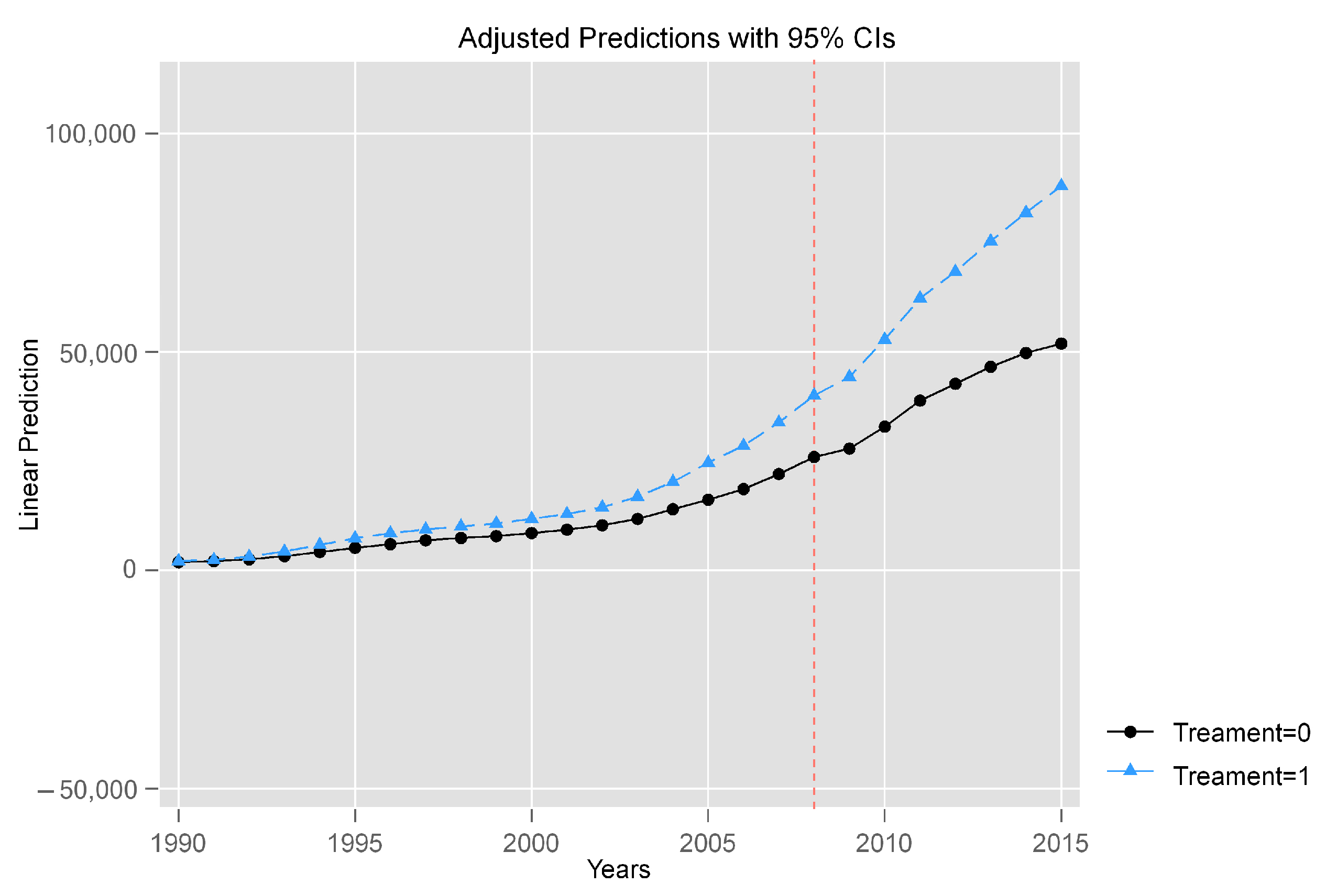
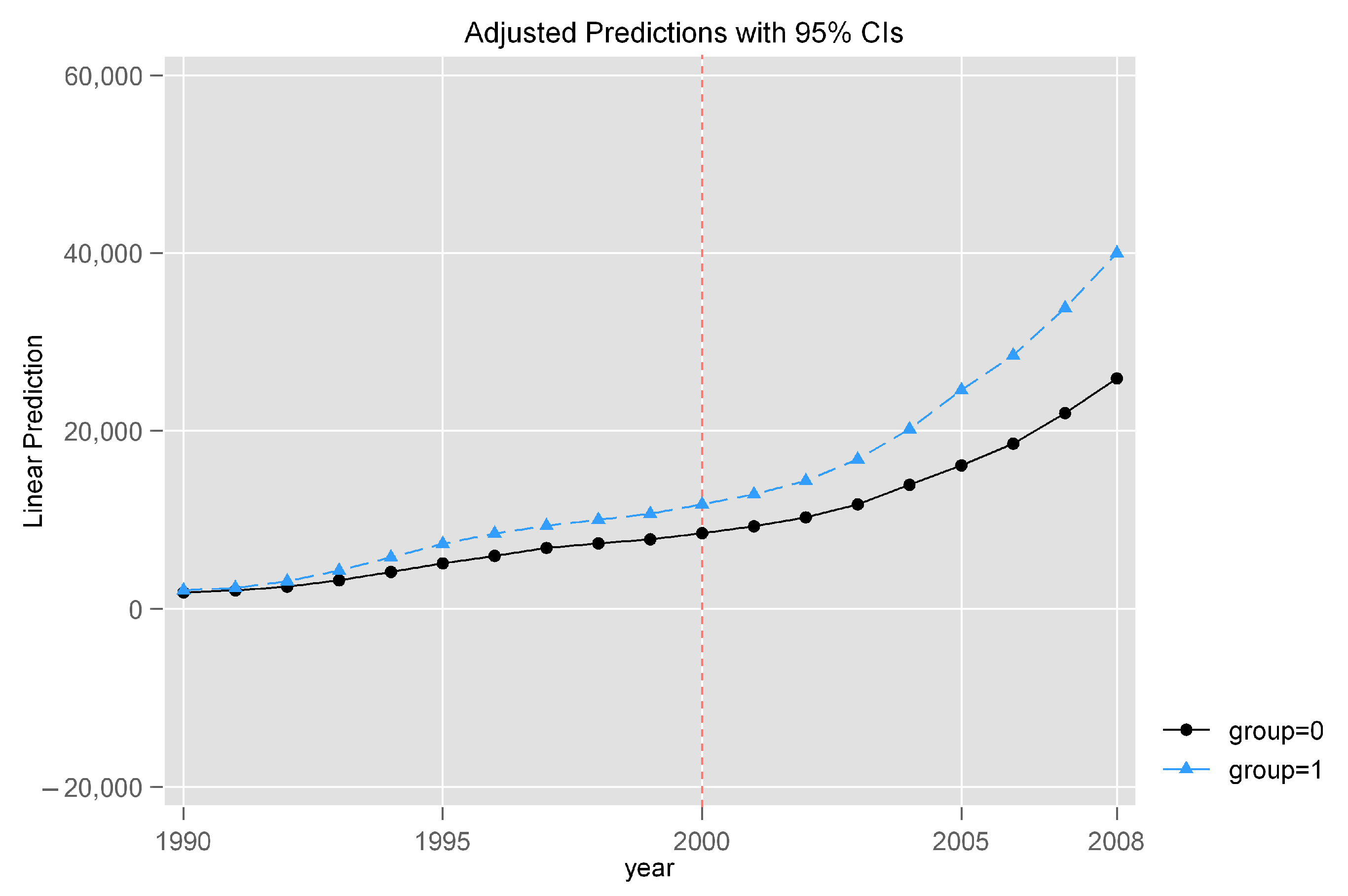
4.2. Results of Difference-in-Differences Design

4.2.1. Baseline Results

Figure 23 shows the parallel trend assumption before the normalisation of cross-strait relations. The remaining provinces are able to generate a valid counterfactual for Jiangsu province as a comparison group based on parallel trends. The baseline results of the difference-in-differences design are visualised in Figure 24. The upper panel presents the highest GDP per capita in Jiangsu province across the remaining provinces. The lower panel shows the per capita GDP growth in the comparison groups over time. The GDP gap per capita between Jiangsu province and the comparison group is significantly greater than the constant gap before 2008. The rest of the provinces in the comparison groups undergo a slight increase after treatment.

Table 4. Did normalised cross-strait relations promote Jiangsu’s economic growth? Yes.

Per Capita GDP	Coef.	p > |t|	[95% Conf. Interval]
Group	3843.73 (3019.27)	0.2	−2083.18	9770.65
Treatment	13,814.79 (1638.51)	0	10,598.35	17,031.24
Diff-in-diff	20,726.52 (5443.07)	0	10,041.61	31,411.42
Year	1306.89 (100.21)	0	1110.17	1503.61
Constant	−2,603,081 (200,273.20)	0	−2,996,223	−2,209,939
Adj R-squared	0.6104
R-squared	0.6101
N	780
F (4, 565)	310.05

reports the evidence for the main results of DiD model. The coefficient of the treatment variable, 13,814.79, is the estimated mean difference in GDP per capita between Jiangsu province and the rest of the control group before the intervention. It illustrates the ‘baseline’ differences between the groups before the intervention was applied to the control group. The estimated ATT of the DiD design is CNY 20,726.52 [95% CI, 10,041.61 to 31,411.42], with a p-value of 0 (0.05), compared with the comparison group by 2015, which is statistically significant. A positive estimate of the ‘treatment’ coefficient (13,814.79) indicates that the normalisation of cross-strait relations had a positive impact on per capita GDP in Jiangsu province. The growth of per capita GDP increased to CNY 1300 per year due to the normalisation of cross-strait relations. The difference-in-differences estimator further supports the hypothesis that regional stability can affect economic development, particularly in areas with close economic cooperation and trading relationships. The results are visualised in Figure 23 and Figure 24.

Figure 25 reports the trajectories of per capita GDP growth in Jiangsu province. Figure 26 visualises the change in the gap in GDP per capita between Jiangsu province and the comparison group in both the pre-intervention and post-intervention periods. From these results, it can be concluded that there is a significant increase in GDP per capita, by almost CNY 20,726.52, in Jiangsu province, after the normalisation of the political relationship between Taiwan and mainland China.

4.2.2. Robustness Test 1: Reassignment of the Treatment

To test whether these findings are unique to the period of 2008, a placebo test was conducted in which the treatment was reallocated to 2000. The treatment—the normalisation of political relations—was reassigned to the year 2000, during the pre-treatment period, 8 years earlier than the treatment actually occurred. In Figure 27, the GDP per capita trajectory in Jiangsu province is still parallel with the comparison group. The gap between the treated unit and the comparison units did not undergo a significant change. Namely, the 2000 placebo did not affect Jiangsu province.

Figure 28 shows the result obtained when data for the post-intervention period is dropped, with the per capita GDP trajectories merely specifying the period between 1990 and 2008, thus reporting the results more clearly: there is no significant change in the per capita GDP gap before and after 2000.

Table 5. Did the normalisation of cross-strait relations in 2000 promote Jiangsu’s economic growth? No.

Per Capita GDP	Coef.	p > |t|	[95% Conf. Interval]
Group	1664.10 (2534.69)	0.512	−3314.46	6642.65
Treatment	2420.75 (1327.86)	0.069	−5028.89	187.39
Diff-in-diff	5739.87 (3682.81)	0.12	−1493.81	12,973.54
Year	1357.05 (120.53)	0	1120.31	1593.78
Constant	−2,701,936 (240,397)	0	−3,174,117	−2,229,755
Adj R-squared	0.4073
R-squared	0.4115
N	570
F (4, 565)	98.75

presents the results obtained using DiD, CNY 5739.865 [95% CI, −1493.809 to 12,973.54], with a p-value of 0.12 (0.1), which is statistically insignificant. In conclusion, the results of the placebo test in which the normalisation of cross-strait relations occurred in 2000 are insignificant.

4.2.3. Robustness Test 2: Spatial Placebo

Similar to the placebo test employed with the synthetic control method, the increase in GDP per capita may not only exist in Jiangsu province. Some provinces might experience a similar increase in economic growth. Thus, a spatial placebo test was conducted in which a comparison province was randomly assigned to be the treated unit. The results are plotted in Figure 29, where the red dot refers to Jiangsu province. It is obvious that Jiangsu province is statistically different from the distribution of the rest of the provinces, at a level of 10% (3/10 = 0.1).

4.2.4. Robustness Test 3: Alternative Samples in the Comparison Group

The western provinces have economic trajectories that diverge greatly from those of the eastern provinces, especially from that of Jiangsu province, which has experienced advanced economic growth. This divergence might lead to many biases in estimation, especially regarding the validity of the parallel trend assumption. Additionally, estimates may not be robust when changing the comparison group. In this robustness test, only the eastern and middle provinces are retained in the comparison group in order to check the sensitivity of the baseline result. Figure 30 shows the parallel trend of this robustness test.

Table 6. Did the normalisation of cross-strait relations promote Jiangsu’s economic growth? Yes.

Per Capita GDP	Coef.	p > |t|	[95% Conf. Interval]
Group	1343.37 (3462.76)	0.698	5463.56	8150.30
Treatment	14,656.94 (2548.52)	0	9647.17	19,666.70
Diff-in-diff	15,737.62 (6242.58)	0.012	3466.25	28,008.90
Year	1625.875 (154.98)	0	1321.22	1930.53
Constant	−3,238,065 (309,735.50)	0	−3,846,928	−2,629,201
Adj R-squared	0.6309
R-squared	0.6345
N	416
F (4, 565)	178.34

presents the results of the DiD estimate, CNY 15,737.62 [95% CI, 3466.25 to 28,008.99], with a p-value of 0.012 (0.05), which is statistically significant. A positive estimate of the ‘treatment’ coefficient (14,656.94) indicates that the normalisation of cross-strait relations had positive impact on per capita GDP in Jiangsu province. Additionally, the DiD estimate remains significant after excluding the western provinces from the comparison group. The results are still robust, and changing the comparison group did not affect the findings of the baseline results. The growth in per capita GDP was found to increase to CNY 1600 per year as a result of the normalisation of cross-strait relations, which is similar to the baseline result. A positive estimate of the ‘treatment’ coefficient (14,656.94) indicates that the normalisation of cross-strait relations had a positive impact on per capita GDP in Jiangsu province.

In analysing the evidence from these results, there are several key points that are worth highlighting. The overall results are robust. The strength of the evidence for or against the hypothesis (i.e., the positive impact of normalised cross-strait relations on regional economic development) varies between the different robustness and placebo tests. The baseline model provides the strongest evidence for this positive impact. The main empirical results indicate that after the normalisation cross-strait relations by means of a series of policy and institutional changes in 2008, Jiangsu province, with close economic connections with Taiwan, experienced significant economic development in terms of per capita GDP. This finding is consistent with the theory and frameworks discussed in Section 2.2. Policy and institutions play an important role in fostering positive economic cooperation and growth changes. The free trade agreement, political statements, and the resumption of communications sent positive signals to businesspeople and private industries, likely increasing their confidence in economic cooperation and integration. The following section will continue the discussion of the results and findings and analyse how these results respond to contemporary literature and move forward with the current debates.

5. Discussion

This section recalls the theoretical framework and the position of this research in the extensive literature in order to discuss how the quality of international political relations might affect economics via different mechanisms. From an empirical perspective, how the findings from this research could be applied in the field of international political economy will be analysed. The study limitations and possible future directions of study are discussed at the end.

5.1. Recollection of Theories

This research discusses the macro-political climate that affects regional economics and presents an overview of the mechanisms and mediators in regional political economies. As discussed in the existing theoretical frameworks, different mechanisms result in a diversity of lenses through which to investigate the manner in which the quality of international political relations affects (regional) economics among countries. The policy and institutions framework and political economy signal models were discussed to explain the causal relationship between normalised political relations and regional economic growth in the case of cross-strait relations. Coalescent political and economic institutions, such as the SEF, ARATS and the Ministry of Economic Affairs (MOEA), are important institutions facilitating trade and investment across the Taiwan Strait. Since the resumption of contact between SEF and ARATS, these institutions have become new gates and offer protection for the stability of capital flow and the safety of business operations. Free trade agreements have also become a driver in opening up further economic cooperation opportunities and removing tariffs. These regulations have increased regional income and promoted regional economic growth by allowing a more free flow of capital and goods. These forms of institutionalised protection and support have provided a platform for economic negotiation and economic policymaking. The increase in GDP per capita in those regions—Jiangsu province in this case—closely engaging with cross-strait trading and investment can serve as proof.

The normalised political relationship between Taiwan and the mainland is bilateral, and is a signal of rapprochement across the Taiwan Strait. The previously restrained economic policies towards the mainland and periodic conflicts under the DPP regime provide a comparison scenario for the normalised political relations under the Ma presidency. The uncertainty of cross-strait confrontation complicates disputes in Asia Pacific. How these confrontations influence regional economic integration and the potential of economic growth matters, especially with the growing economic impact of East Asia. The Ma administration conveyed the political signal that, contrary to the previous confrontational attitude, the Taiwanese government would like to generate mutual trust and remove the political tension across the Taiwan Strait, which was a preliminary step towards deeper economic integration. This was also a signal indicating a safe environment for trade and investments. This study argues that policies, institutions and the sending of positive political signals through improving the linkages between regions subject to confrontation are able to sustain commercial confidence and minimise military conflict under capricious environments—in this case, in the context of cross-strait relations. Also, reduced confrontation and political stability are multidimensional and manifest in varied ways and areas. It is important to highlight the importance of investigating different dimensions of changes in political relations, ranging from policies, institutions and informal/formal signals across sectors and regions. Through analysis of these theoretical connections and mechanisms, the results obtained using the synthetic control method and difference-in-differences are convincing: normalised cross-strait relations did indeed exert a positive economic influence on regional economics.

5.2. Empirical Implications

Better international political relationships usually encourage interstate free trade agreements and infrastructure construction in temporal environments that are free of political conflict. This finding endorses the idea that stable political ties with less confrontation could promote economic growth and a more intimate commercial link between the cooperating countries. If the government emphasises commercial interests in its policy implications, adopting a compromised and soft foreign policy approach could be better. Diplomacy carried out by talking softly and carrying a small stick will spare more space for international commercial cooperation and regional integration, especially for countries with strong economic complementarity. Unfortunately, sullen and uncompromising strategies do not work in either country’s favour, locking the liberalisation of trade and investment in a stalemate. The globalised market and the trend of regional integration require at least periodic peace in the regions, which plays an important role in the international commercial chain. This research suggests that policymakers should make a balanced decision to achieve both their political and economic interests. These compromises in the face of political gridlock could result in a win–win situation for the participating countries.

Normalised cross-strait relations after long-term confrontation is the situation in the East Asia region. This could have policy implications and serve as a cost reference for countries facing similar dilemmas, such as North Korea and South Korea. Resuming bilateral contact might lead to a chain of economic reactions. In Asia, many regional and interstate conflicts, especially peace on the Korean peninsula and the Taiwan Strait are closely related to economic integration in the Asia-Pacific region. If changes of political relations on the Korean peninsula are consistent with these findings, better political relations between North Korea and South Korea might result in better economic integration and cooperation.

Political relations between countries/regions can be either a roadblock or an accelerant to economic growth. East Asia has been an important region for global peace and economic development. The complicated and unpredictable political relations between different countries/regions in Asia have been important in influencing the sustainability and stability of economic growth. Even with increasing economic integration, periodic conflict and military threats still threaten the stable development of the economy, especially the relations between mainland China and Japan, North Korea and South Korea, South Korea and Japan, and Taiwan and mainland China. A number of different political conflicts exist in Asia, for example, the issues regarding the South Sea territory between the Philippines, Vietnam, and mainland China, and the recognition of the history between Korea and Japan. These fluctuating factors in political relations between countries/regions an unpredictably influence economic exchanges and capital inflows. The confrontation between Taiwan and the mainland further complicates stable economic exchange and trade and is a potential timebomb in the Asia-Pacific region. Therefore, it is important to acknowledge how international and regional political relations have affected regional economics and integration. In turn, sustainable economic integration could bring these regions temporary or long-term peace.

5.3. Limitation and Future Studies

Even though this research has strengths in terms of measuring the impact of political stability and revealing casual relationships, it also has several limitations. Regarding the methodology, both methods offer rigorous models to measure the effect with concrete evidence. However, the research design does not make it possible to test the parallel trends assumption in difference-in-differences. If this assumption is invalid, the estimates in DiD will be biased. From the results displayed in the previous section, for both the baseline results and placebo tests, it can be seen that the actual treated unit and the synthetic one almost always achieved a close match across the pre-intervention periods. Although this research included fixed investments as a ratio to control the possible confounding effects in the difference-in-differences methods, because different investment policies in different regions still influence these provinces differently, difference-in-differences might not capture all of the potential effects that may influence the outcome variables. To address this concern, the synthetic control method in this study has provided a better alternative for evaluating the validity of the research results. The synthetic control method does not require this constant time assumption to guarantee the accuracy of the estimates (O’Neill et al. 2016). For the synthetic control method, it is more important that the treated unit achieves a well-fitted match in the pre-intervention periods with the synthetic counterpart, and the results robustly show a good match.

As for the selection of indicators, per capita GDP is a direct but quite general indicator. Extensive variables obtained from microdata could be further included by using other, more robust statistical methodologies to extend the research lenses. Trade and investment mainly focus on specific industries, for example, high-tech or labour-intensive industries. Significant variations exist among different investment types, industries, talent transfer, and employment opportunities. This research should provide a full-scale picture of these variations. GDP is a very direct, but one-dimensional indicator. The cost–benefit relationship may not be as positive as we think. The loss of enterprise responsibility of Taiwanese business people on the mainland, tax exemption, and pollution issues could cause long-term damage, which cannot be evaluated purely on the basis of per capita GDP indicators. In the selection of the treatment units, the other comparison regions, for example, Shanghai and Fujian, do not mean that they received no treatment. This does not mean that the normalisation of cross-strait relations has not affected them. This research design mainly focused on the most significant effect for measuring the economic impact of political relations. Therefore, the full-scale impact might have been unavoidably neglected.

Whilst this research infers possible mechanisms connecting normalised political relations and regional economic growth, these mechanisms failed to be specified in these two methodologies. The theoretical frameworks provided a wide range of possible mechanisms, and these mechanisms could be inferred from the hints in the historical reviews on the political economy of Taiwan–China relations. However, these hints can only provide possible links and explanations as to how the normalisation of political relations has resulted in regional economic growth. Which linkages and mediators exactly are the mechanisms, or whether all of these theoretical frameworks could constitute credible explanations, remains uncertain. It is possible that not all regions would experience the same pattern, and that not all mediators can link the quality of interstate political relations to regional economics. This is also a limitation of this research. In further studies, more appropriate mechanisms and mediators could be tested, helping to uncover the exact functioning mediators in the linkage of the international political economy.

In addition, politics and economics have different development logics. Personal recognition of political issues can greatly determine ideologies within mainstream society (Balliet et al. 2018). The political relationships between Taiwan and mainland China are much more complicated than economic cooperation. More importantly, trade and investment between Taiwan and mainland China have been restrained by the political tension between the two countries, and there will still be many uncertainties in the future. Looking back through history, even though the short-term formal contact in 1992–1993 alleviated the political tension in cross-strait relations, it did not bring about long-lasting peace in the Taiwan Strait. The current literature still needs to answer the question as to whether the normalisation of cross-strait relations since 2008 could deliver a long-lasting effect on bettering the economic relationship between the two sides. Further studies could also evaluate the long-term and temporal economic influence of the previous government of President Ma in the shadow of the current governance of the DPP.

President Ma Ying-jeou adopted a diplomatic truce to seek more chances in international organisations, providing Taiwan with more economic development space. This research was primarily focused on the regional economic effect of the normalisation of political relations in mainland China and overlooked its multidimensional influence on both sides. Regional economic changes will be multilateral, affecting both Taiwan and mainland China. This empirical research focused mainly on mainland China’s economic impact, overlooking the possible impact on Taiwan. It would be more comprehensive if the economic conditions in Taiwan were also investigated. Taiwan and mainland China share different systems and economic structures, and thus, mainland China and Taiwan might experience different impacts and economic shocks in different sectors and regions. Further comparisons could justify further study from this perspective.

From a broader perspective, this research focused on the impact of the normalisation of cross-strait relations while not accommodating the more comprehensive political multilateral relations and po-litical pressure imposed from other countries outside East Asia in the models. The effect of the normalisation of cross-strait relations on economic growth is likely the result of multilateral relations among Taiwan, the mainland, and other countries due to the need for economic cooperation and a peaceful Asia-Pacific environment. The one-directional research between political relations and economic growth unavoidably overlooks the complexity of the inextricable relationship between these two variables. The impact of normalised cross-strait relations on regional economic growth has been leveraged by international marketisation, the commitment of the WTO, and growing regional integration. These exogenous factors have gradually pulled economic cooperation across the Taiwan Strait into free trade and investment trajectories.

6. Conclusions

This research can serve as an insightful reference for countries/regions trapped in complicated domestic and international political conditions, showing how a stable and positive political relationship can influence economic growth under particular conditions. This research argues that when there is constant economic exchange, the normalisation of political relations positively promotes economic growth and strengthens economic ties. This research reports robust evidence that the normalisation of cross-strait relations led to a nearly 7% yearly increase in regional per capita GDP in Jiangsu province, compared with provinces with little or less economic exchange across the Taiwan Strait. The results obtained using both the synthetic control method and the difference-in-differences are robust to different specifications and placebo studies, including alternative sample pools, placebo–time treatment, and spillover specification. With the difference-in-differences design, there was an average increase in per capita GDP annually of CNY 2960.93 (GBP 336.47), with a 95% confidence interval with a lower bound of CNY 1434.52 yuan (GBP 163.01) and an upper bound of CNY 4487.35 yuan (GBP 509.93). The results from the synthetic control method show that if there had been no normalisation of cross-strait relations in 2008, the possibility of achieving such a large per capita GDP in Jiangsu province would have been 0.033. The normalisation of cross-strait relations brought a 6.5% annual per capita GDP (approximately 2500 yuan) increase in Jiangsu province, compared to the counterfactual in the absence of normalised cross-strait relations.

This research argues that better political relations after periodic military threats and conflicts have a significant economic impact in regions involving intimate bilateral trade and investments. This result reports the empirical evidence against the previous hypothesis of ‘integrative and disintegrative aspects’ (Harding 1993) regarding cross-strait relations. ‘Divergent politics and interdependent economics’ (Kastner 2007, p. 668) are no longer the reality in the Taiwan Strait since the normalisation of cross-strait relations. Economic interactions on both sides involve complicated interests and a capricious globalised market. The States make their foreign policies based on the calculation of both political and commercial interests. The economic interactions on both sides involve complicated interests and a capricious globalised market. Taiwan Strait is still a flash point in East Asia. The rise of China’s comprehensive power and Taiwan’s hesitation to institutionalise the economic relationship provide unique cases for academic exploration (Leng 2017). 2008 was a watershed and a critical junction for mainland China-Taiwan relations, from a very confrontational level to a less confrontational and peace-orientated level. However, the normalisation of cross-strait relations does not equate to the disappearance of rooted and uncompromised conflicts. Politicised ideology and unification issues are still rooted in the cross-strait relations, which cannot be addressed immediately. The evolution of cross-strait relations has involved capricious domestic and complicated international politics. The question of how cross-strait links will affect regional economics could have an open-ended answer in different periods, particularly after Tsai Ing-wen’s presidency and after DDP became the majority ruling party in 2016.

This investigation of the political economy of cross-strait relations was, in any case, a case study. The results are possibly limited by the fact that both confrontational countries/regions have strong economic complementarity, and this complementarity has been partly exploited. The relationship between political relations and economics is quite dynamic, and its correlations may be contradictory at different points in time. Poor political relations do not necessarily lead to the end of economic integration and growth in regions involving international trade and investments. The positive or negative correlations between political relations and regional economic growth vary in different situations. Taiwan’s investment and trade restrictions towards the mainland suppress the economic potential of both sides, which makes the economic impact of normalised political relations more significant. This suppression provides a development space for the subsequent burgeoning of free trade and investment. If political conflicts were alleviated, this condition would provide a positive model for regional integration, similar to the European Union, which promotes both economic and political integration, ultimately building up innumerable links based on economic exchanges.

References

1. Abadie, Alberto. 2005. Semiparametric Difference-in-Differences Estimators. Review of Economic Studies 72: 1–19. [Google Scholar] [CrossRef]
2. Abadie, Alberto, Alexis Diamond, and Jens Hainmueller. 2010. Synthetic control methods for comparative case studies: Estimating the effect of California’s tobacco control program. Journal of the American Statistical Association 105: 493–505. [Google Scholar] [CrossRef]
3. Abadie, Alberto, Alexis Diamond, and Jens Hainmueller. 2015. Comparative politics and the synthetic control method. American Journal of Political Science 59: 495–510. [Google Scholar] [CrossRef]
4. Abadie, Alberto, and Jens Gardeazabal. 2003. The economic costs of conflict: A case study of the Basque Country. American Economic Review 93: 113–32. [Google Scholar] [CrossRef]
5. Abdella, Ahmed Berhan, Naghavi Navaz, and Fah Benjamin Chan Yin. 2018. The effect of corruption, trade openness and political stability on foreign direct investment: Empirical evidence from BRIC countries. International Journal of Advanced and Applied Sciences 5: 32–38. [Google Scholar] [CrossRef]
6. Acemoglu, Daron, Simon Johnson, Amir Kermani, James Kwak, and Todd Mitton. 2013. The Value of Connections in Turbulent Times: Evidence from the United States. National Bureau of Economic Research 121: 368–391. [Google Scholar]
7. Aisen, Ari, and Francisco Jose Veiga. 2013. How does political instability affect economic growth? European Journal of Political Economy 29: 151–67. [Google Scholar] [CrossRef]
8. Angrist, Joshu, and Jörn-Steffen Pischke. 2009. Mostly Harmless Econometrics: An Empiricist’s Companion. Princeton: Princeton University Press. [Google Scholar]
9. Baier, Scott, Jeffrey Bergstrand, and Michael Feng. 2014. Economic integration agreements and the margins of international trade. Journal of International Economics 93: 339–50. [Google Scholar] [CrossRef]
10. Balliet, Daniel, Joshua Tybur, Junhui Wu, Christian Antonellis, and Paul Van Lange. 2018. Political Ideology, Trust, and Cooperation: In-group Favoritism among Republicans and Democrats during a US National Election. The Journal of Conflict Resolution 62: 797–818. [Google Scholar] [CrossRef]
11. Barbieri, Katherine. 2003. Models and Measures in Trade-Conflict Research. In Economic Interdependence and International Conflict: New Perspectives on an Enduring Debate. Edited by Edward D. Mansfield and Brian M. Pollins. Ann Arbor: University of Michigan Press, pp. 207–21. [Google Scholar]
12. Beck, Thorsten, George Clarke, Alberto Groff, Philip Keefer, and Patrick Walsh. 2001. New tools in comparative political economy: The database of political institutions. The World Bank Economic Review 15: 165–76. [Google Scholar] [CrossRef]
13. Beine, Michel, and Serge Coulombe. 2007. Economic integration and the diversification of regional exports: Evidence from the Canadian–US Free Trade Agreement. Journal of Economic Geography 7: 93–111. [Google Scholar]
14. Berger, Daniel, William Easterly, Nathan Nunn, and Shanker Satyanath. 2013. Commercial imperialism? Political influence and trade during the Cold War. American Economic Review 103: 863–96. [Google Scholar] [CrossRef]
15. Bolt, Paul J. 2001. Economic Ties Across the Taiwan Strait: Buying Time for Compromise. Issues and Studies 37: 80–105. [Google Scholar]
16. Brzezinski, Zbigniew, and John J. Mearsheimer. 2005. Debate: Clash of the Titans. Foreign Policy 146: 46–50. [Google Scholar]
17. Busse, Matthias, and Carsten Hefeker. 2007. Political risk, institutions and foreign direct investment. European Journal of Political Economy 23: 397–415. [Google Scholar]
18. Cai, Kelvin G. 2011. Cross-Taiwan Straits Relations Since 1979 Policy Adjustment and Institutional Change across the Straits, Singapore. Hackensack: World Scientific. [Google Scholar]
19. Chase, Michael, Kevin Pollpeter, and James Mulvenon. 2004. Shanghaied? The Economic and Political Implication of the Flow of Information Technology and Investment across the Taiwan Strait. Technical Report 133. Santa Monica: RAND Corporation. [Google Scholar]
20. Chen, Dean P. 2013. The Strategic Implications of Ma Ying-jeou’s “One ROC, Two Areas” Policy on Cross-Strait Relations. American Journal of Chinese Studies 20: 23–41. [Google Scholar]
21. Chen, Xiangming. 2018. Globalisation redux: Can China’s inside-out strategy catalyse economic development and integration across its Asian borderlands and beyond? Cambridge Journal of Regions, Economy and Society 11: 35–58. [Google Scholar] [CrossRef]
22. Chen, Xin. 2014. On the Interactive Route and Pattern of the Cross-Strait Economic and Political Relations. Journal of Beijing Union University (Humanities and Social Sciences) 12: 48–53. (In Chinese). [Google Scholar]
23. Cheung, Gordon C. K. 2007. China Factors: Political Perspectives and Economic Interactions. New Brunswick: Transaction Publishers. [Google Scholar]
24. Chiu, Lee-in Chen. 2016. The pattern and impact of Taiwan’s investment in mainland China. In Emerging Patterns of East Asian Investment in China: From Korea, Taiwan and Hong Kong. London: Routledge, pp. 143–65. [Google Scholar]
25. Chu, Yun-Han. 1997. The Political Economy of Taiwan’s Mainland Policy. Journal of Contemporary China 6: 229–57. [Google Scholar] [CrossRef]
26. Clarke, P. 2008. Does Growing Economic Interdependence Reduce the Potential for Conflict in the China-Taiwan-U.S. Triangle? American Journal of Chinese Studies 15: 57–68. [Google Scholar]
27. Conable, Barber B., Jr., and David M. Lampton. 1993. China: The coming power. Foreign Affairs 72: 145. [Google Scholar] [CrossRef]
28. Corrado, Germana. 2020. Institutional quality and access to financial services: Evidence from European transition economies. Journal of Economic Studies 47: 1363–76. [Google Scholar] [CrossRef]
29. Davis, Patricia A. 1999. The Art of Economic Persuasion: Positive Incentives and German Economic Diplomacy. Ann Arbor: University of Michigan Press. [Google Scholar]
30. Dent, Christopher. 2005. Taiwan and the New Regional Political Economy of East Asia. The China Quarterly 182: 385–406. [Google Scholar] [CrossRef]
31. Dittmer, Lowell. 2017. Taiwan and China: Fitful Embrace. California: University of California Press. [Google Scholar]
32. Ekanayake, E. M., A. Mukherjee, and B. Veeramacheneni. 2010. Trade blocks and the gravity model: A study of economic integration among Asian developing countries. Journal of Economic Integration 25: 627–43. [Google Scholar] [CrossRef]
33. Frank, R. 2006. The political economy of sanctions against North Korea. Asian Perspective 30: 5–36. [Google Scholar] [CrossRef]
34. George, Alexander L., and Andrew F. Bennett. 2004. Case Studies and Theory Development in the Social Sciences. Singapore: MIT. [Google Scholar]
35. Gören, Erkan. 2014. How ethnic diversity affects economic growth. World Development 59: 275–97. [Google Scholar] [CrossRef]
36. Gowa, Joanne, and Raymond Hicks. 2017. Commerce and Conflict: New Data about the Great War. British Journal of Political Science 47: 653–74. [Google Scholar] [CrossRef]
37. Hall, C. Michael. 2005. Territorial economic integration and globalisation. In Tourism in the Age of Globalisation. London: Routledge, pp. 36–58. [Google Scholar]
38. Han, Baran. 2021. Secondary sanctions mechanism revisited: The case of US sanctions against North Korea. In Research Handbook on Economic Sanctions. Cheltenham: Edward Elgar Publishing, pp. 223–237. [Google Scholar]
39. Harding, Harry. 1993. The Concept of “Greater China”: Themes, Variations and Reservations. The China Quarterly 136: 660–86. [Google Scholar] [CrossRef]
40. Hart, Jeffrey A., and Joan Edelman Spero. 2013. The Politics of International Economic Relations. London: Routledge. [Google Scholar]
41. Hasan, M. Aynul. 1999. Conceptual framework for growth triangles. (International Trade)(Report). Pakistan Development Review 38: 805–22. [Google Scholar] [CrossRef]
42. Hayakawa, Kazunobu, Fukunari Kimura, and Hyun-Hoon Lee. 2013. How does country risk matter for foreign direct investment? The Developing Economies 51: 60–78. [Google Scholar] [CrossRef]
43. Heo, Uk, and Wondeuk Cho. 2012. The Economic Cooperation Framework Agreement between China and Taiwan and Its Implications for South Korea. Pacific Focus 27: 205–34. [Google Scholar] [CrossRef]
44. Hong, Tsai-Lung, and Chih-Hai Yang. 2011. The economic cooperation framework agreement between China and Taiwan: Understanding its economics and politics. Asian Economic Papers 10: 79–96. [Google Scholar] [CrossRef]
45. Hung, Tzu-Chieh. 2017. Rethinking Public Diplomacy: A Study of China Exerting its Influence on Taiwan. Doctoral dissertation, Waseda University, Tokyo, Japan. [Google Scholar]
46. Imai, Kosuke. 2017. Quantitative Social Science. An Introduction. Princeton: Princeton University Press. [Google Scholar]
47. Jeong, Bora, and Hoon Lee. 2021. US–China commercial rivalry, great war and middle powers. International Area Studies Review 24: 135–48. [Google Scholar] [CrossRef]
48. Jong-A-Pin, R. 2009. On the measurement of political instability and its impact on economic growth. European Journal of Political Economy 25: 15–29. [Google Scholar] [CrossRef]
49. Kastner, Scott. 2007. When Do Conflicting Political Relations Affect International Trade? Journal of Conflict Resolution 51: 664–88. [Google Scholar] [CrossRef]
50. Keshk, Omar M. G., Brian M. Pollins, and Rafael Reuveny. 2004. Trade still follows the flag: The primacy of politics in a simultaneous model of interdependence and armed conflict. Journal of Politics 66: 1155–79. [Google Scholar] [CrossRef]
51. Kim, Hyung Min, and David L. Rousseau. 2005. The classical liberals were half right (or half wrong): New tests of the “liberal peace,” 1960–88. Journal of Peace Research 42: 523–43. [Google Scholar] [CrossRef]
52. Koo, Min Gyo. 2009. The Senkaku/Diaoyu dispute and Sino-Japanese political-economic relations: Cold politics and hot economics? The Pacific Review 22: 205–32. [Google Scholar] [CrossRef]
53. Leng, Tse-Kang. 2017. Cross-Strait Economic Relations and China’s Rise: The Case of the IT Sector. In Taiwan and China: Fitful Embrace. Edited by L. Dittmer. Oakland: University of California Press, pp. 151–75. [Google Scholar]
54. Li, Yuhua, Ze Jian, Wei Tian, and Laixun Zhao. 2021. How political conflicts distort bilateral trade: Firm-level evidence from China. Journal of Economic Behavior & Organization 183: 233–49. [Google Scholar]
55. Libman, Alexander, and Evgeny Vinokurov. 2012. Regional integration and economic convergence in the Post-Soviet space: Experience of the decade of growth. JCMS: Journal of Common Market Studies 50: 112–28. [Google Scholar] [CrossRef]
56. Lijphart, Arend. 1971. Comparative Politics and the Comparative Method. The American Political Science Review 65: 682–93. [Google Scholar] [CrossRef]
57. Lin, Justin Yifu, Xifang Sun, and Ye Jiang. 2013. Endowment, industrial structure, and appropriate financial structure: A new structural economics perspective. Journal of Economic Policy Reform 16: 109–22. [Google Scholar] [CrossRef]
58. Liu, Weidong, and Michael Dunford. 2016. Inclusive globalization: Unpacking China’s belt and road initiative. Area Development and Policy 1: 323–40. [Google Scholar] [CrossRef]
59. Long, Andrew G. 2003. Does trade follow peace? Post-war bilateral trade and expectations for recurrent conflict. Paper presented at the Annual Meeting of the American Political Science Association, Philadelphia, PA, USA, August 28–31. [Google Scholar]
60. Lupo Pasini, F. 2013. Economic stability and economic governance in the Euro Area: What the European Crisis can teach on the limits of Economic integration. Journal of International Economic Law 16: 211–56. [Google Scholar] [CrossRef]
61. Mamoon, Dawood, and S. Mansoob Murshed. 2010. The conflict mitigating effects of trade in the India-Pakistan case. Economics of Governance 11: 145–67. [Google Scholar] [CrossRef]
62. Mansfield, Edward D., Jon C. Pevehouse, and David. H. Bearce. 2014. Preferential trading arrangements and military disputes. In Power and the Purse. London: Routledge, pp. 92–118. [Google Scholar]
63. Mattoo, Aaditya, Randeep Rathindran, and Arvind Subramanian. 2001. Measuring Services Trade Liberalization and Its Impact on Economic Growth: An Illustration. Washington, DC: World Bank Publications, vol. 2655. [Google Scholar]
64. Najafi, Amir, and Hossein Askari. 2012. The Impact of Political Relations Between Countries on Economic Relations. PSL Quarterly Review 65: 247–73. [Google Scholar]
65. O’Neill, Stephen, Noémi Kreif, Richard Grieve, Matthew Sutton, and Jasjeet S. Sekhon. 2016. Estimating causal effects: Considering three alternatives to difference-in-differences estimation. Health Services and Outcomes Research Methodology 16: 1–21. [Google Scholar] [CrossRef]
66. Obadić, Ivan. 2017. In Pursuit of Stability: Yugoslavia and Western European Economic Integration, 1948–1970. Doctoral dissertation, European University Institute, Fiesole, Italy. [Google Scholar]
67. Pasara, Michael Takudzwa. 2020. An overview of the obstacles to the African economic integration process in view of the African continental free trade area. Africa Review 12: 1–17. [Google Scholar] [CrossRef]
68. Piccolino, Giulia. 2020. Regional integration. In The Routledge Handbook of EU-Africa Relations. London: Routledge, pp. 188–201. [Google Scholar]
69. Pietrangeli, Giulia. 2016. Supporting regional integration and cooperation worldwide: An overview of the European Union approach. In The EU and World Regionalism. London: Routledge, pp. 9–43. [Google Scholar]
70. Rashid, Mamunur, Xuan Hui Looi, and Shao Jye Wong. 2017. Political stability and FDI in the most competitive Asia Pacific countries. Journal of Financial Economic Policy 9: 140–55. [Google Scholar] [CrossRef]
71. Ryan, Andrew M., James F. Burgess Jr., and Justin B. Dimick. 2015. Why We Should Not Be Indifferent to Specification Choices for Difference-in-Differences. Health Services Research 50: 1211–35. [Google Scholar] [CrossRef]
72. Sabir, Samina, and Ahsan Khan. 2018. Impact of political stability and human capital on foreign direct investment in East Asia & Pacific and south Asian countries. Asian Journal of Economic Modelling 6: 245–56. [Google Scholar]
73. Shambaugh, David. 2008. International Relations of Asia. Lanham: Rowan and Littlefield. [Google Scholar]
74. Shee, Poon Kim. 2004. The political economy of Mahathir’s China policy: Economic cooperation, political and strategic ambivalence. Ritsumeikan Annual Review of International Studies 3: 59–79. [Google Scholar]
75. Simmons, Beth A. 2005. Rules over real estate: Trade, territorial conflict, and international borders as an institution. Journal of Conflict Resolution 49: 823–48. [Google Scholar] [CrossRef]
76. Snyder, Scott. 2009. China’s Rise and the Two Koreas: Politics, Economics, Security. Boulder: Lynne Rienner. [Google Scholar]
77. Sutter, Karen M. 2002. Business Dynamism across the Taiwan Strait: The Implications for Cross-Strait Relations. Asian Survey 42: 522–40. [Google Scholar] [CrossRef]
78. Swank, Duane. 2002. Global Capital, Political Institutions, and Policy Change in Developed Welfare States. Cambridge: Cambridge University Press. [Google Scholar]
79. Tavares, Rodrigo, and Vanessa Tang. 2016. Regional Economic Integration in Africa: Impediments to Progress? In Comparative Regionalisms for Development in the 21st Century. London: Routledge, pp. 209–32. [Google Scholar]
80. Tsai, Chung-min. 2017. The Nature and Trend of Taiwanese Investment in China (1991–2014): Business Orientation, Profit Seeking, and Depoliticization. In Taiwan and China: Fitful Embrace. Edited by Lowell Dittmer. Oakland: University of California Press, pp. 133–50. [Google Scholar]
81. Tsai, Tung-Chieh, and Tongy Tai-ting Liu. 2017. Cross-Strait Relations and Regional Integration: A Review of the Ma Ying-jeou Era (2008–2016). Journal of Current Chinese Affairs 46: 11–35. [Google Scholar] [CrossRef]
82. Tung, Hans H., and Yun-Han Chu. 2015. Signalling peace: A theory of the ECFA and a peace dividend beyond the Taiwan Strait. In Taiwan and the ‘China Impact’. London: Routledge, pp. 128–47. [Google Scholar]
83. Yahuda, Michael. 2012. The International Politics of the Asia Pacific. London: Routledge. [Google Scholar]
84. Yang, Chyan, and Shiu-Wan Hung. 2003. Taiwan’s dilemma across the Strait: Lifting the ban on semiconductor investment in China. Asian Survey 43: 681–96. [Google Scholar] [CrossRef]
85. Yang, Yung-Lieh, Tsui-Yueh Cho, and Ming-Hsiang Huang. 2017. Impacts of the economic cooperation framework agreement on banking cost efficiency in China and Taiwan a stochastic metafrontier approach. Hitotsubashi Journal of Economics 58: 121–41. [Google Scholar]
86. Yu, Jingwen, and Chunchao Wong. 2011. Political Environment and Economic Development: Analysis Based on the Evolution of Cross-Strait Relations. South China Economics 4: 31–39. (In Chinese). [Google Scholar]
87. Zhang, Baohui. 2011. Taiwan’s New Grand Strategy. Journal of Contemporary China 20: 269–85. [Google Scholar] [CrossRef]
Figure 1. Direct investment by Taiwan in mainland China from 1991 to 2015. Source: Investment Commission, MoMA, ROC, at <http://www.moeaic.gov.tw/chinese/>, accessed on 3 September 2022.
Socsci 12 00493 g001
Figure 2. The number of agreements signed through ARATS and SEF. Data source: Adapted from the authors of the Mainland Affairs Council, Straits Exchange Foundation, and Chen (2018, pp. 2–3), at <https://www.mac.gov.tw/cp.aspx?n=1494D59CE74DF095>, accessed on 8 August 2023.
Socsci 12 00493 g002
Figure 3. The number of meetings between ARATS and SEF. Data source: Adapted from the authors of the Mainland Affairs Council, Straits Exchange Foundation, and Chen (2018, pp. 2–3), at <https://www.mac.gov.tw/cp.aspx?n=1494D59CE74DF095>, accessed on 8 August 2023.
Socsci 12 00493 g003
Figure 4. Approved investment flowing into Jiangsu province. Source: Overseas Chinese and Foreign Investment Commission, Taiwan, https://www.moeaic.gov.tw/english/news_bsAn.jsp, Taiwan Yearly Investment Report 2015 (accessed on 8 August 2023).
Socsci 12 00493 g004
Figure 5. Amount of direct investments made by Taiwan and amount of investment received by Jiangsu province. Source: Overseas Chinese and Foreign Investment Commission, Taiwan, https://www.moeaic.gov.tw/english/news_bsAn.jsp, Taiwan Yearly Investment Report 2015.
Socsci 12 00493 g005
Figure 6. Parallel trends before 2008 (with covariates).
Socsci 12 00493 g006
Figure 7. Parallel trends before 2008 (without covariates).
Socsci 12 00493 g007
Figure 8. Average GDP of Jiangsu province and the rest provinces.
Socsci 12 00493 g008
Figure 9. Trends in per capita GDP: Jiangsu and synthetic Jiangsu.
Socsci 12 00493 g009
Figure 10. The GDP gap between Jiangsu and synthetic Jiangsu.
Socsci 12 00493 g010
Figure 11. Trends in per capita GDP: Jiangsu and synthetic Jiangsu (spillover test).
Socsci 12 00493 g011
Figure 12. The gap between the GDP per capita and synthetic GDP per capita for all provinces (Jiangsu highlighted as the orange line and the rest provinces as grey lines).
Socsci 12 00493 g012
Figure 16. Ratio of post-intervention RMSPE to pre-intervention RMSPE: Jiangsu province and comparison provinces (Jiangsu highlighted in red).
Socsci 12 00493 g016
Figure 17. Normalisation of political relations occurring in 2000: trends in GDP in Jiangsu and synthetic Jiangsu.
Socsci 12 00493 g017
Figure 18. Trends of the per capita GDP of Shandong province and synthetic Shandong province.
Socsci 12 00493 g018
Figure 20. Trends of the per capita GDP of Jiangsu and synthetic Jiangsu.
Socsci 12 00493 g020
Figure 21. Trends of the per capita GDP of Jiangsu and synthetic Jiangsu.
Socsci 12 00493 g021
Figure 22. Trends of the per capita GDP of Jiangsu and synthetic Jiangsu.
Socsci 12 00493 g022
Figure 23. Parallel trends before 2008 (without covariates).
Socsci 12 00493 g023
Figure 24. Parallel trends and baseline results (without covariates).
Socsci 12 00493 g024
Figure 25. Trajectory of GDP per capita in Jiangsu province.
Socsci 12 00493 g025
Figure 26. Adjusted prediction of economic growth in Jiangsu province. Note: The prediction of DiD is surrounded by 95% confidence intervals.
Socsci 12 00493 g026
Figure 27. Normalisation of cross-strait relations occurring in 2000 (1990–2015).
Socsci 12 00493 g027
Figure 28. Normalisation of cross-strait relations occurring in 2000 (1990–2008).
Socsci 12 00493 g028
Figure 29. DiD estimates of the distribution of all provinces (Jiangsu highlighted in red).
Socsci 12 00493 g029
Figure 30. Parallel trends between Jiangsu province and the comparison group.
Socsci 12 00493 g030