Education and Crime across America: Inequity’s Cost

Abstract

Much of current research on crime and education has focused on the effect of minimum dropout age on rates of crime. Combining the FBI’s uniform crime reporting database and district finance data, we study the longitudinal relationship between crime in every town/city (whose police department has reported crime statistics) and its school district spending in years 2003 to 2018. We combine over 213 datasets to control for population, density, wealth, education, employment, cost-of-living, race, law enforcement, and voting history. Additionally, we also look at teacher salary, teacher engagement, and student chronic absenteeism. Using linear mixed-effect modeling, we find an overall average of 2.35% percent decrease in property crime for every $1000 more a school district spends per pupil on education. Moreover, a $1000 increase in education spending decreased property crime nearly four times as much as a 10 percent increase in per capita income. We also looked at the range in district spending in towns/cities and counties whose students attend multiple districts. We find that for every $1000 difference in district spending within a city, property crime increases by an average of 3%; interestingly, violent crime decreases by 3%. When we lag variables of education quality, allowing these effects to playout, we also find that for every 10 percentage-point increase in chronic absenteeism among students, violent crime increases by 4%. Importantly, we find no such effect for property crime, suggesting a distinct mechanism of education on violent crime. Additionally, both law enforcement and unemployment explain little variance in crime. Our results demonstrate a robust relationship between education funding and reduced crime across America with regard to amount spent per student as well as equity in spending.

1. Introduction

Often, crime is fought by redoubling enforcement or legislating methods of hopeful deterrence—increasing punishment, enacting mandatory sentencing minimums, and adopting redoubtable, unforgiving laws like “Three Strikes” for repeat offenders, a law that is currently upheld in twenty-two states. While government spending on education increased by a factor of 1.2 from 1980 to 2005, spending on police and law enforcement grew by 1.5-fold. Spending on corrections more than tripled (Lochner 2010).

Still, crime persists, and such hardened approaches have raised questions not only of efficacy, but also of ethics and economics. Imprisoning someone for a year is the monetary equivalent of two semesters at Harvard1, 25% more than what most American households will make in a year2 (AP; Guzman). African American citizens are five times more likely to be incarcerated than their white counterparts, and though black and Latino people make up just one-third of the general population, they constitute over half of imprisoned Americans, a figure that has climbed exponentially from 500,000 people in 1980 to over 2.2 million in 2015. The United States has amassed 21% of the world’s incarcerated, despite comprising just 5% of its population (NAACP 2020). Coincidentally, two-thirds of those incarcerated dropped out of high school (Harlow 2003). In 1995, one-third of black men between the ages of 20 and 29 were either incarcerated, on probation, or on parole (Mauer 2000).

Ultimately, effective methods of crime reduction is an empirical question, and here, we explore that question through the scope of education quality and spending. In addition to equity, there are several practical reasons to focus on crime reduction in youth and adolescence. In 2010, 1.9 million youth between the ages of 15 and 19 were arrested, representing 19% of all arrests, despite assuming only 7% of the population (Mancino et al. 2016). Moreover, numerous studies have demonstrated persistence of criminal activity over time: (Blumstein et al. 1985; Nagin and Paternoster 1991; Nagin and Land 1993; Nagin et al. 1995; Broidy et al. 2003). Thus, the effects can be both immediate, and lasting: stemming the perpetuity of crime into adulthood.

Previous research has found strong negative relationships at micro/macro levels and has focused on years of compulsory education, region, incapacitation, and education level of those arrested. In 1972, England and Wales enacted sweeping legislation mandating an extra compulsory year of high school; Machin et al. (2011) employed discontinuity regression to determine that men who finished high school (between the ages of twenty-one and twenty-five) were eight times less likely to be arrested than those who had dropped out. In the United States, Lochner and Moretti (2004) performed analyses of compulsory education laws among states and estimated that increasing average years of schooling by one year reduces both property and violent crime by 11–12 percent. One Italian study looking at crime on a regional basis concluded that more than seventy-five percent of convicted Italians had not completed high school (Buonanno and Leonida 2006). Waldfogel (1994) and Hjalmarsson (2008) found that lower educational attainment and decreased future earnings correlate with incarceration during adolescence. Similarly, Machin and Meghir (2004) found that decreased wages among low-wage workers lead to an increase in crime. Jacob and Lefgren (2003) and Luallen (2006), looking at teacher in-service days, estimated the effect on crime of being in school on a particular day and found that the level of property crime committed by juveniles decreased by 14 percent on school days but violent crime increased by 28 percent. They attributed to both incapacitation and concentration respectively. Notably, Luallen determined that urban school districts were most affected by incapacitation and found an interaction between incapacitation and differing juvenile criminal histories among students.

On the other hand, some researchers focus on specific longitudinal datasets that provide insight into family background and behavior. Merlo and Wolpin (2008) used data from the 1997 youth cohort of the National Longitudinal Surveys (NLSY97) to explore the relationship between incarceration rates of young adult black males aged 19 to 22 and family background characteristics, as well as juvenile behaviors. They found that the largest difference in incarceration rates arose between black male youths who did not attend school at age 16; non-attenders are 4 times more likely to be incarcerated at ages 19 to 22. Moreover, they also found that those who committed a crime at age 14 were twice as likely to commit a crime at ages 19 to 22. Mancino et al. (2016), incorporated a smaller scale “Pathways to Desistance”, multi-site dataset (n = 1354), where serious adolescent offenders were followed over a seven-year period after enrollment. This study gathered important variables (past education, criminal activity, family criminal history, and cognitive tests) generating a comprehensive picture of life events, better suited to understanding the dynamics between crime and education in addition to roles of state dependence, returns to experience, and heterogeneity. Specifically and importantly, this dataset allowed for the study of serious offenders. Mancino et al. found small effects of experience and stronger evidence of state dependence and heterogeneity for crime and schooling, and concluded that policies affecting individual heterogeneity (emotional/social skills), and those extricating youth from crime, can have important and lasting effects despite the accumulation of previous criminal experience.

While reviewing compulsory laws, teacher in-service days, and years of education can uncover important effects of incapacitation and education attainment on crime, we seek to establish a mechanism by which investment in children through the gestalt of quality education (spending is a proxy albeit an imperfect one) decreases crime. Like Mancino et al. (2016) and Merlo and Wolpin (2008), we use a longitudinal dataset to look at education spending alongside its corresponding year’s crime values and as a lagged variable (5-years) to disentangle effects of incapacitation with the development of life-skills, like increased patience and risk aversion (Becker and Mulligan 1997) or through an increase in earning potential because of extra time spent in school (“income effect”). Our unit of analysis is a place (which, for purposes here, is essentially a town or city). Additionally, we look at instructional wages (as a proportion of total spending), teacher retention, teacher absenteeism, and percent chronic absenteeism of students. Through these variables we deepen our empirical approach to determine whether spending differs substantially from other variables, demonstrating the value of teachers (proportion of total spending) and engagement of those teachers (proportion teachers absent for more than 10 days during the school year). Lastly, we use chronic absenteeism not only as a proxy of school quality (better schools keep students engaged), but also to explore the idea of incapacitation: controlling for other factors, one would expect greater crime in places with increased rates of chronic absenteeism.

Surprisingly, we could not find a single paper that looks specifically at education spending and crime. In his paper looking at increased arrest rates appearing to reduce crime, Levitt and Miles (2007) do include education spending per capita (distinctly different from per pupil) as a nuisance variable among categories of Murder, Rape, Robbery, Assault, Burglary, Larceny, and Auto Theft and reports effect sizes of −3.07, −0.48, −0.67, −1.85, −0.83, −1.18, −1.39 (with p-values 0.1 or below). His study considers several nuisance variables of 59 large cities from 1970 to 1992. Other studies looking at education spending do not consider crime. Jackson et al. (2016) incorporated an instrumental variable of state- by-state court-mandated school finance reforms, revealing that a 10% increase in per pupil spending each year for all 12 years of public school lead to a 0.31 increase in completed years of education, roughly 7% higher wages, and a 3.2 percentage point reduction in the annual incidence of adult poverty. These effects were more pronounced for children from low-income families. In his comprehensive paper, “Does School Spending Matter?” Jackson (2020) culls school spending studies. Of those specifically looking at multiple states, he finds that 12 of those 13 studies discern a positive and statistically significant relationship between school spending and student outcomes. Looking at single-state studies, Jackson breaks these into unrestricted spending, textbook spending, capital and construction spending, and Title 1 spending. He finds that 13 of the 20 studies examining within state (or city within state) funding found positive and significant relationships between spending and student outcomes. None found negative and significant impacts.

Collating 213 datasets over a sixteen-year period (2003 to 2018), we scrutinize the relationship of school district per pupil spending on the crime rates of its cities and towns. We explore covariates of population, population density, per capita income, median income, proportion of children living in poverty, unemployment rate, cost-of-living (median rent), voting history, race, educational attainment, and the amount of law enforcement in these towns and cities.

2. Data

Our compiled dataset comprises data from the Small Area Income and Poverty Estimates Program (SAIPE), the National Center for Education Statistics (NCES) (2019), Education Demographic and Geographic Estimates (EDGE), Civil Rights Data Collection (CRDC), Missouri Mable (Missouri Census Data Center 2019), the American Community Survey (ACS), Annual Survey of School System Finances, the Decennial Census, MIT Election Data (MIT Election Lab 2019) and Science Lab, United States Department of Justice (2019a) and ICPSR, and the FBI’s Uniform Crime Reporting Program (UCR). We provide summary statistics for this data in Supplementary Materials S1, and we supplement this paper with an in-depth guide to how we aligned these datasets (Supplementary Materials S2).

2.1. Education Spending Data

We use the Annual Survey of School System Finances (2003 through 2018), a branch of the Census, for school district financial information. We reconcile the overlap among some places with multiple counties by using only the crime values for the corresponding county in which the population of the place predominantly exists. Additionally, given that elementary school districts overlap secondary school districts (and are also a primary source for consolidation and reduction in overall school districts) both of which potentially overlap cities and counties (unified school districts can also overlap counties), we employ only data from unified school districts—districts serving kindergarten through 12th grade. In total, there are 10,479 unified school districts.

After filtering non-unified school districts and recalculating student expenditures, we removed all school districts with fewer than fifty enrolled students. This removed 346 observations, leaving us with a maximum student expenditure of $53,000 per year. We had thirty-six observations below $40,000 down to $289 in Wilmington, Vermont. Before choosing any cutoff minimum, we inspected the veracity of these outliers. Furthermore, we performed a secondary screening of the data to verify the accuracy of extant anomalies in a school district’s year to year education spending over the 15-year period. We created a function in R to group individual school districts and look at whether extremes existed within this window. We scrutinized all values with an absolute difference greater than $3000 from the preceding year. We identified 400 school districts with an absolute difference greater than $3000. We retained anomalous values unless we could otherwise locate more sufficient values either at the school district’s website or on the corresponding state’s Department of Education website (U.S. Department of Education 2021). We replaced 59 values. This practice shifted the max from $53,000 down to $47,000. Given that places could attend multiple school districts, we averaged school district spending by place. However, we attempted to maintain the existing variation by creating separate models looking at both mean and range expenditure values (among places and counties).

We determined which places attended which districts using the NCES “School District Geographic Relationship Files” from 2013 through 2018 to link places and county subdivisions with districts and used the Missouri MABLE 2000 dataset to link places with districts from before that time (see Supplementary Materials for specifics).

Additionally, we used the Annual Survey of School System Finances to obtain the proportion of instructional wages to total spending. We pulled teacher retention and absenteeism and student chronic absenteeism from the Civil Rights Data Collection.

2.2. Crime Data

After removing values flagged by the FBI, we had 127,344 distinct crime observations from 2003 through 2018, for corresponding police departments which reported crime. The UCR did not publish data in 2004 for cities under 10,000. In the Supplementary Materials, we discuss in detail how we maximized the number of crime values. It is important to note here that these UCR FBI values only exist at the level of a city/town police department. Thus, there is no way to look at violent and property crime in different areas or neighborhoods of a city. We discuss this in more depth at the end of our paper.

Filtering out non-unified school districts, we winnowed total crime observations to 104,240. Because FBI UCR datasets only include state and city names (and in some cases, county names), joining FBI crime datasets with Census datasets (U.S. Census Bureau 2019a, 2019b, 2019c, 2019d, 2019e, 2019f, 2019g, 2019h, 2000a, 2000b) was laborious. Misspellings or additional qualifiers (town, village, etc.) prevent crime observations from joining with expenditure datasets. Thus, we preserved as many values as possible by using the anti-join (Wickham et al. 2019) feature in R to see which values didn’t overlap between datasets. We then cut supplementary words like “metropolitan”, “borough”, etc. from city/town names. We preserved county subdivision values by creating a parallel dataset and joining this dataset with police department information. We then ran a district check to ensure no duplicate district values.

2.3. Other Data

We used 4 datasets for population values (Decennial census: 2000, 2010; Population Estimates Program); 16 datasets for proportion children in poverty (Small Area Income and Poverty Estimates, SAIPE, Program: 2003–2018); 1 dataset for presidential elections (MIT Election Data + Science Lab: 2000–2016); 30 law enforcement datasets (United States Department of Justice (2019b) and FBI, LEOKA police employee data: 2003, 2016, not yet published for 2017 and after; and UCR FBI, police employee data: 2003–2018). For the following covariates, we obtained datasets for both places and county subdivisions totaling 20 datasets for education attainment (Decennial: 2000; ACS 5-year estimates: 2010–2018); 20 datasets for median income (Decennial: 2000; ACS 5-year estimates: 2010–2018); 22 datasets for per capita income (Decennial: 2000; ACS 5-year estimates: 2009–2018); 22 datasets for unemployment rate information (Decennial: 2000; ACS 5-year estimates: 2009–2018); 20 datasets for housing costs (Decennial: 2000; ACS 5-year estimates: 2010–2018); 6 datasets for race variables (Decennial: 2000; ACS 5-year estimates: 2010, 2015); and 5 datasets from the CRDC.

3. Methodology

In OLS, endogeneity poses a problem given its presence in the error term; in a standard OLS regression, it is likely to be correlated with independent variables and thus, there will not be zero covariance between the error term and independent variables (Levacic et al. 2005). Fixed effect models are also more likely to overfit the data given that all observations are pulled from separate distributions. While there is an assumption of independence, this assumption does not hold: naturally, it would make sense that crime in Chicago in 2005 would be correlated with crime in Chicago in 2006 (unless there exists an exogenous variable driving this change). While instrumental variables offer important conclusions; they also come with their own caveats and controversy and pose a problem for an analysis of this scope. One must identify an instrument that correlates with education spending but not with crime. Education spending is affected by wealth, which inevitably affects where one lives, where one attends school, whether there is an increase in independent/private schools, the dominant political party, and crime rate. We used multi-level, mixed-effect models. There are several distinct advantages of multilevel modeling: (1) the “shrinking” of estimates toward a group-level mean reducing chances of overfitting; (2) The ease with which grouped data can be nested (3) missing data are assumed to be missing at random (MAR) and not missing completely at random (MCAR), a much less elastic assumption.

In a multilevel time-series model, at the lowest, repeated measures level, we have:

Y_ti = β_0i + β_1iT_ti + β_2iX_ti + e_ti

where Y_ti is the crime for town/city i at year t, T_ti is a time indicator for the specific year and X_ti is a time-varying predictor variable. This lowest level captures individual variability over time (intra-individual change), and thus, the intercept β_0i and slope β_1iT_ti vary across cities/towns. The time indicator is 0 … 15 (though we’ve centered time in our actual model) for the years 2003–2017.

The second level explains variability between cities and towns (inter-individual differences)

β_0i = γ₀₀ + γ₀₁Z_i + u_0i
β_1i = γ₁₀ + γ₁₁Z_i + u_1i

where γ represents fixed effects and u represents random effects (capturing individual variation). β_0i captures variability in the intercept (the crime values in 2003), where u_0i is each city/town’s intercept’s distance from the mean, and β_1i captures variability in the slope (change in crime values over time), and thus, u_1i represents each city/town’s individual rate of change in crime from the mean slope. Z_i represents a time invariant covariate (for instance, geographical location); these do not exist in our model.

Thus, naturally, one can expand our model by the addition of time-varying covariates (carrying a ti component) at the first level as:

Crime_ti = β_0i + β_1iYear_ti + β_2i Population_ti + β_3i Population density_ti + β_4i Per capita income_ti + β_5i Education
spending_ti + β6i White_ti + β_7i Voting history_ti + β_8i Black_ti + β_9i Median Rent_ti + β_10i Bachelors_ti + β_11i
Proportion children in poverty_ti + β_12i Asian_ti + β_13i High school diploma_ti + β_14i Law Enforcement_ti + β_15i No
high school diploma_ti + e_ti + u₀ + u_1i

However, the real benefit of multilevel models is the ease with which one can then create new levels of nested data. Certainly, crime and education funding among cities also depends on the counties and states in which they reside (some states provide more funding; or in instances like Vermont, education funding is redistributed among towns/cities; or in many Southern states, public school funding can be reallocated to private schools). This dependence can be accounted for in a multilevel model.

γ₀₀ = δ₀₀₀+ u₀₀
γ₁₀ = δ₁₀₀+ u₁₀

and thus, in adding county as a random effect, we create a third level and a model that expands to

Crime_tij = β_0ij + β_1ijYear_tij + β_2ij Population_tij + β_3ijPopulation density_tij … β_15ij No high school diploma_tij + e_ti + u₀ + u_1i

and the addition of a fourth level, state, which expands the model to

Crime_tijk = β_0ijk + β_1ijkYear_tijk + β_2ijk Population_tijk + β_3ijkPopulation density_tijk … β_15ijk No high school diploma_tijk + e_ti + u₀ + u_1i

Each crime value then corresponds to a timepoint t for a specific town/city (i), in a specific county (j) nested within a specific state (k). The only difference between the above and our model is that rather than including time as a fixed effect, we include it as a random slope; hence the u1i. For our later models, crime count becomes the dependent variable, and the type of crime becomes a dummy variable, and thus takes the form

Count_tijk = β_0ijk + β_1ijkYear_tijk + β_2ijk Crime_tijk + β_3ijk Population_tijk + β_4ijkPopulation density_tijk … β_15ijk No high school diploma_tijk + e_ti + u₀ + u_1i

We smoothed crime values by adding a constant of 1 (one cannot use a natural logarithm here given that there are crime rates of 0) and cross-validated our final model using root mean squared error (RMSE) of predicted 2018 crime values with actual observed 2018 crime values from UCR data. We do this for both the total crime model and then for the property and violent crime models, including interactions. As stated in our results, our models were constructed first by their comparative impact on AIC, such that, in establishing effect sizes, we had already considered their predictive robustness.

For proportion instructional spending, we then looked at whether the school districts that increased in instructional spending proportion demonstrated different crime trends than those that did not. We lagged education spending such that we could compare it to the previous year and filtered all values less than the previous year. To limit noise, we then winnowed this dataset to only those cities/towns that had increased proportional instruction spending over at least eight of the fifteen years. Mostly small towns and cities remained (N = 296) with comparatively low violent crime that wavered over the fifteen-year period, seemingly emblematic of a sample of smaller places susceptible to extremes. Ultimately, we ended up not using the proportion instructional spending here, nor the CRDC teacher retention data given the oddities (values with greater than 1 for a proportion, etc., and the retention data comprised only 8000 values, a fraction of our dataset.)

Lastly, we decided to impute missing data vs delete missing values. Comparatively few values were missing, and this appeared to not be at random—smaller towns and cities (those with fewer crimes) were more likely to have missing values; deleting these would have introduced bias, so imputation was the lesser of two evils. (See Supplementary Materials S1 & S3). We used the Multivariate Imputation by Chained Equations package (Van Buuren and Groothuis-Oudshoorn 2011) and maintained the multilevel structure of the data. Our law enforcement variable of officers was missing nearly 2.5 times the number of values (16.7% total) as any other variable; this was despite our combining of two separate police employee datasets from separate sources (FBI and National Archive of Criminal Justice Data 2020). Except for our total crime and crime type models at the place level, where we sought RMSE values and merged the missing data into one complete dataset, we imputed 20 data points for each missing value (Graham et al. 2007) and then analyzed 20 separate datasets to obtain final averaged values via Rubin’s rules for pooling parameter estimates (Rubin 1987).

We implement root mean squared error (RMSE) as a check to ensure that the effect sizes from our models are grounded not only in their own significance but in an overall predictive capacity as well.

4. Results

4.1. Education Spending on Overall Crime

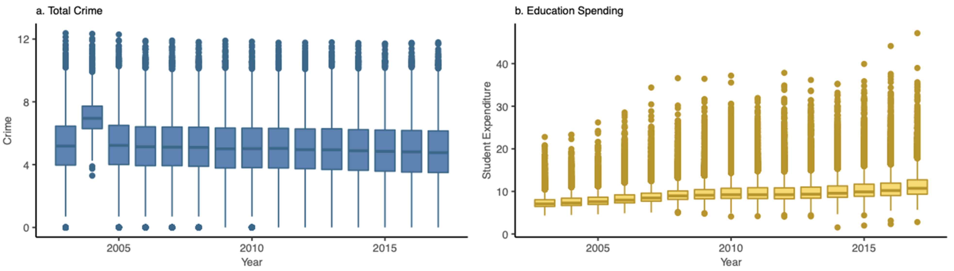
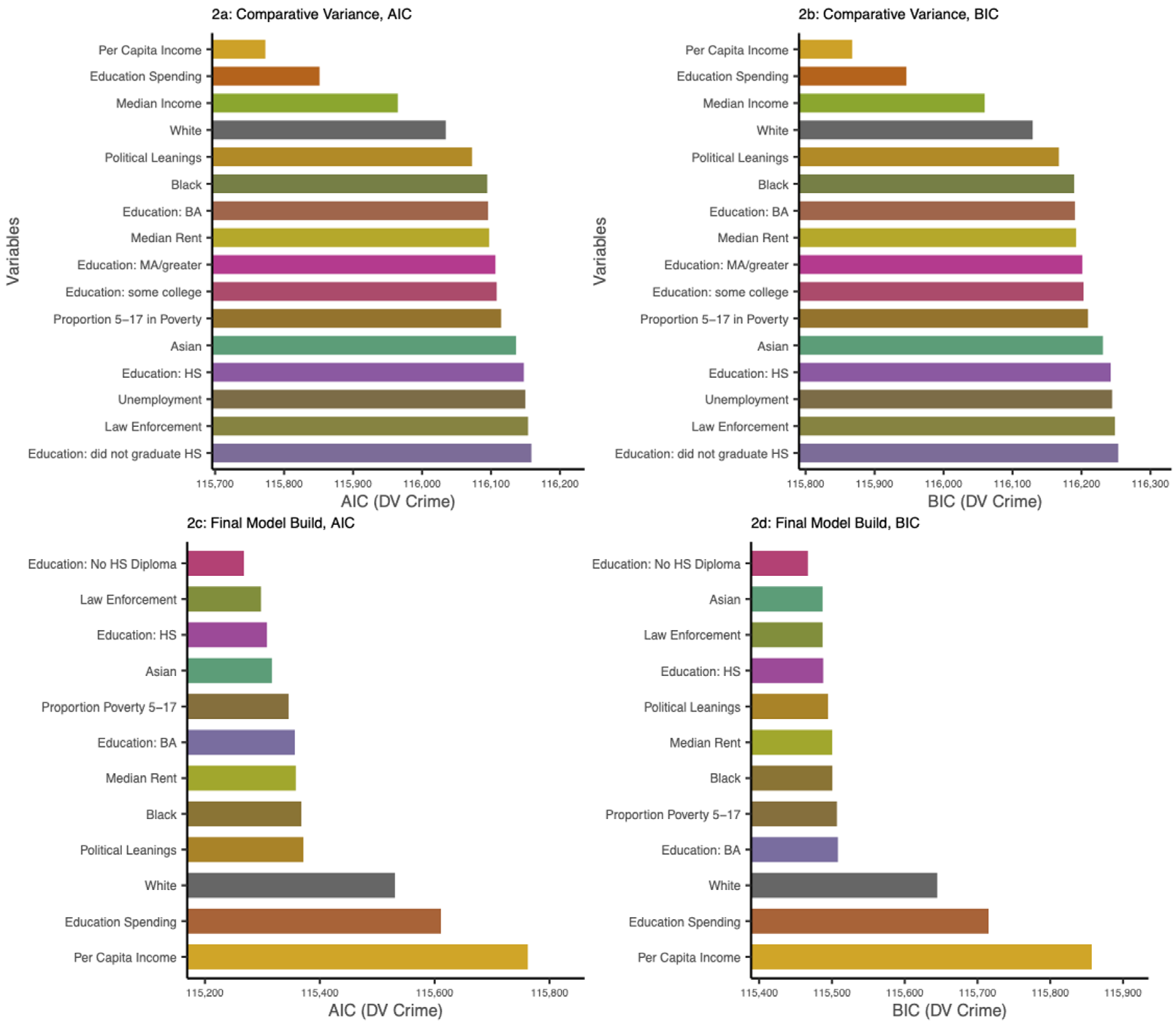
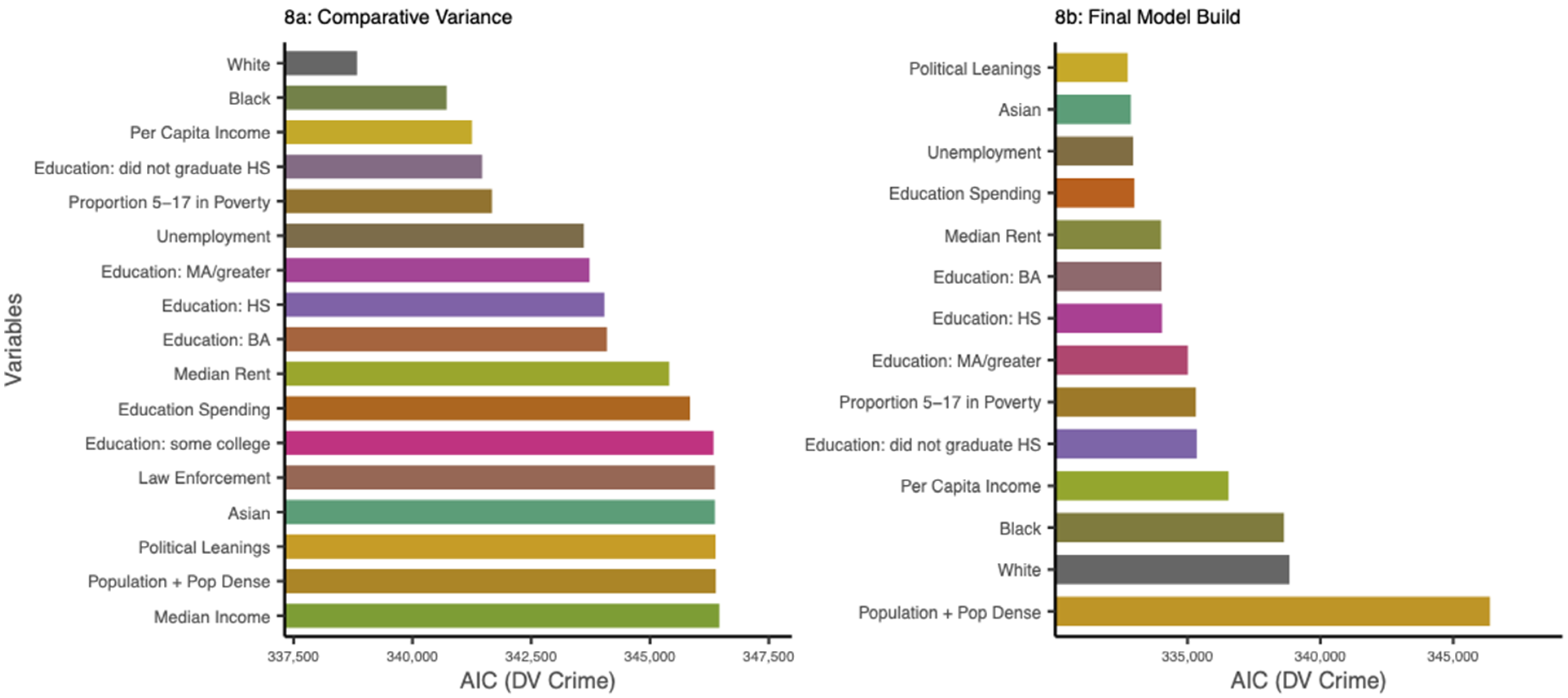
Figure 1 shows how crime and education spending vary from 2003 to 2017. Instead of modeling year as a fixed factor in our mixed effect models, which represents the salient variance across time but not the underlying causes of that variance, we modeled time in years as a random slope to allow for differences in rates of crime change among places over the 15-year period. We added explanatory variables to our crime model in an order informed by the comparative variance they accounted for in models containing only population and population density (detailed in Figure 2a). We modeled place, county, and state as random effects, accounting for the correlation structure of repeated “place” measures over time, and the nesting structure of places within counties and counties within states. We provide both AIC and BIC values in Figure 2.

Our first crime model comprises thirteen variables (Figure 2c), though three of these are race: black, white, and Asian; and three of these are educational attainment: graduated high school, did not graduate high school, and obtained a bachelor’s. The remaining variables are population, population density, education spending, per capita income, median gross rent3 (cost-of-living), voting history (for presidential election years), total law enforcement (number of employed officers), and proportion of 5 to 17-year-olds living in poverty4. 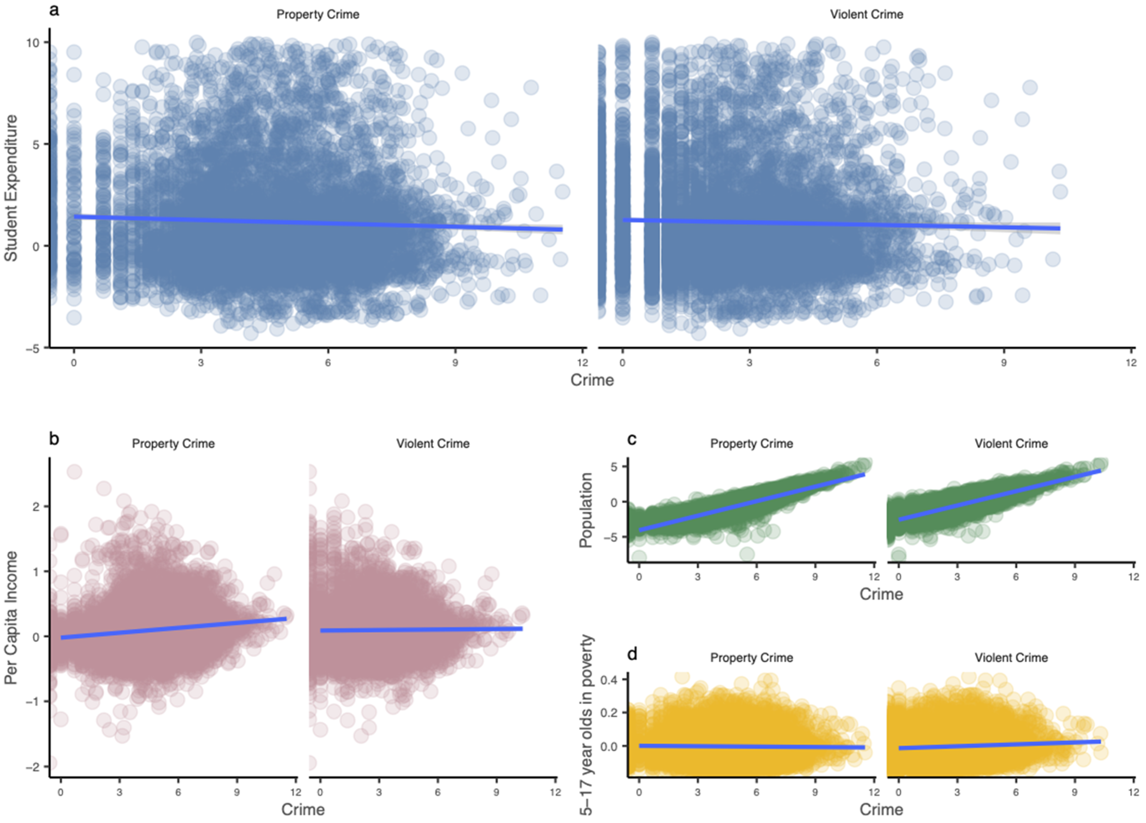In Figure 3 and Figure 4, we have plotted the covariates used in our model. 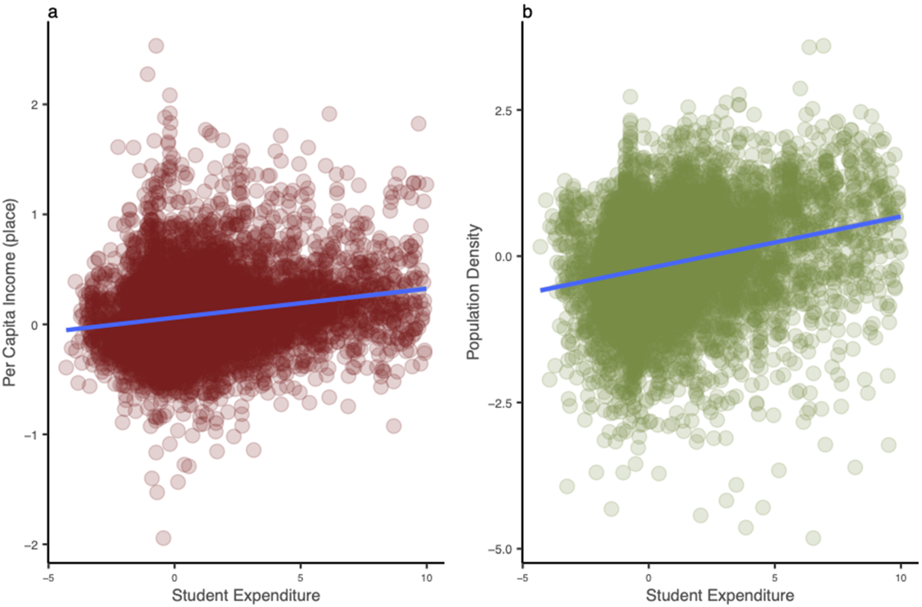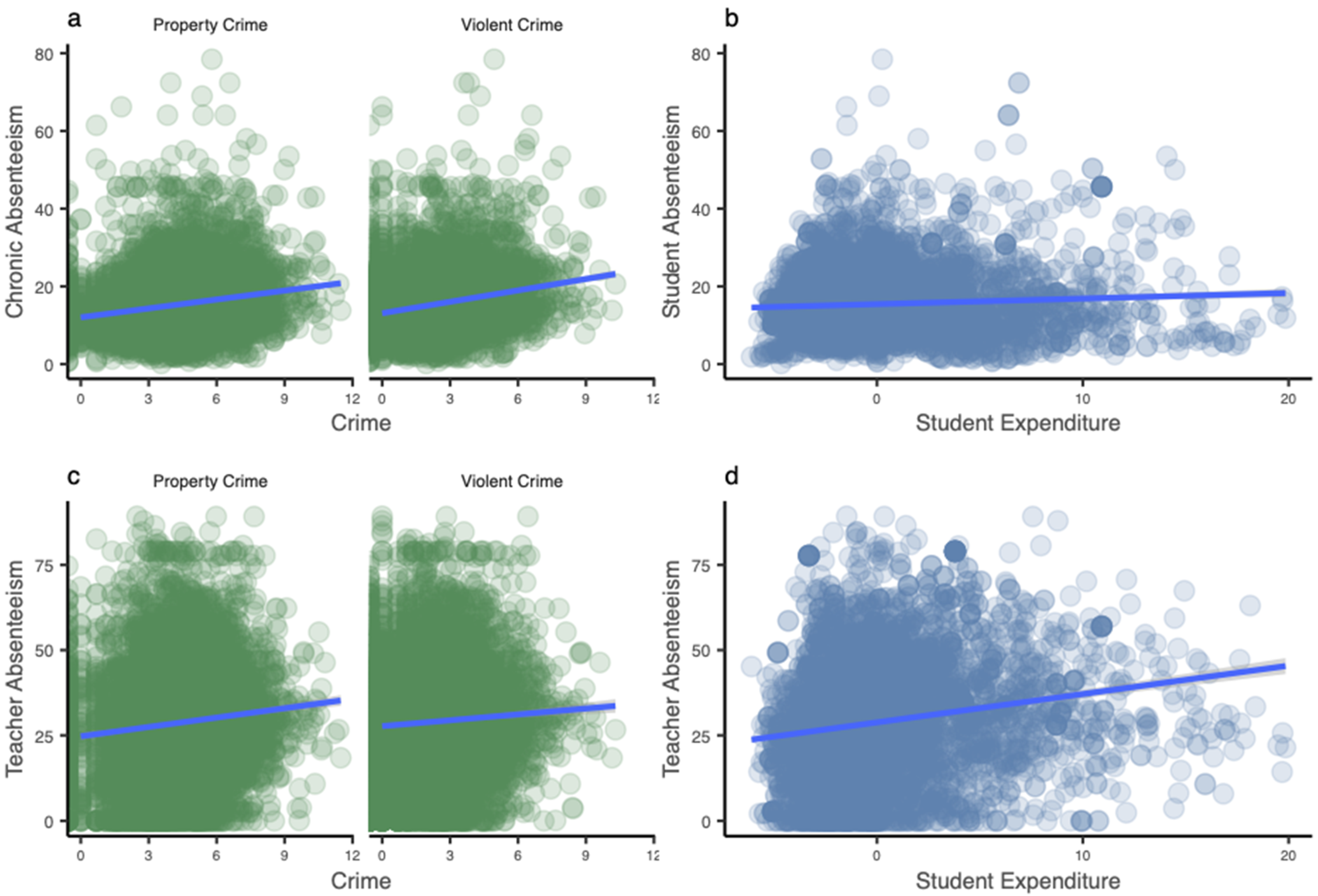Figure 3 shows the relationship between covariates and crime by crime type (property/violent). We graph student expenditure, the main independent variable related to decrease in crime (Figure 3a), in Figure 4, portraying the relationship between education spending and covariates of per capita income and population density (using the final year of data, 20175).

Our first crime model, looking at total crime, began with a null model AIC of 148,719 and decreased to a final model AIC of 115,279 (Figure 2b) and comprises the covariates listed above. Controlling for population and population density, time (year) as a fixed effect with a random slope, decreased the AIC to 114,434. This model captures the total variance in the decline of crime over the fifteen-year period. In this model, crime decreases on average 2.98 ± 0.07 percent each year (2.84, 3.11).

Naturally, crime increases with population: for every ten percent population increase, crime increases an average 12.35 ± 0.06 percent (12.23, 12.47). However, we found an inverse relationship between population density and crime: crime decreases by an average 0.22 ± 0.09 percent (0.04, 0.40).

Our first crime model (Figure 2b) also shows that per capita income and school district expenditure both considerably decreased the AIC, revealing a negative relationship between per pupil spending and crime (Figure 3). For every $1000 more a city spends on education, its crime decreases by an average 2.49 ± 0.14 percent (2.21, 2.77).

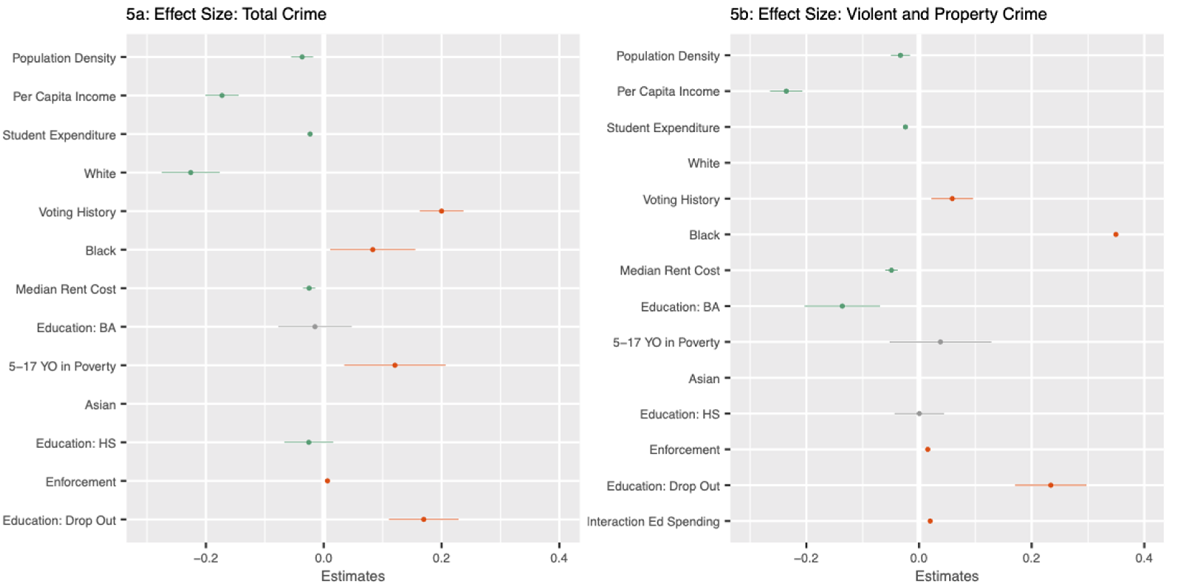
We then add all variables in the order conveyed in Figure 2b. Effect sizes are provided in Figure 5a. There were three variables that were not significant; these were educational attainment variables of having “some college experience” (x²(1, N = 98,600) = 0.33, p = 0.56) and a “master’s degree/greater” (x²(1, N = 98,600) = 3.04, p = 0.08), and unemployment (x²(1, N = 98,600) = 0, p = 1). Notably, we found that for every ten percent increase in per capita income (after controlling for cost-of-living), crime decreases by 1.65 ± 0.14 percent (1.38, 1.92). Additionally, for every ten percentage-point increase in the proportion of 5 to 17-year-olds living in poverty, crime increases by 1.27 ± 0.45 percent (0.39, 2.15). Regarding the impact of race on crime, we find that for every ten percentage-point increase in white constituents of a city or town, its crime decreases by an average 2.03 ± 0.25 percent (1.53, 2.53). For the same ten percentage-point increase in the black constituents of a city or town, its crime will increase by an average 0.68 ± 0.37 percent (−0.05, 1.42), and for Asian constituents of a city or town, 5.15 ± 1.42 percent (2.37, 7.94). There exist a multitude of interactions among race, educational attainment, and wealth; looking at mere total crime is insufficient. 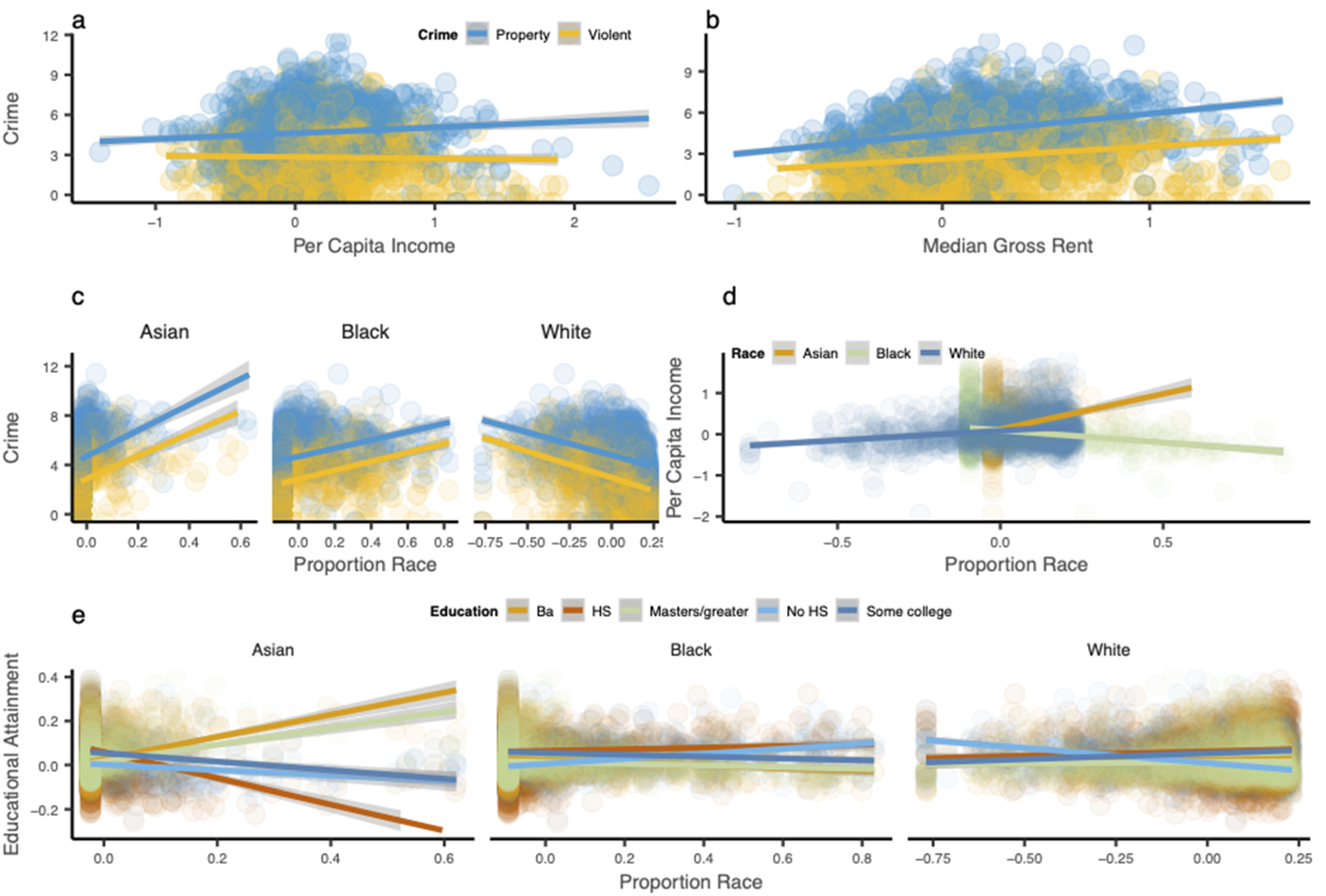In Figure 6a, we demonstrate the interaction between crime type and per capita income—property crime increases, but violent crime decreases. Figure 6b,c show that crime is also affected by cost-of-living since property crime and violent crime (at a slightly slower rate) increase as cost-of-living increases. Figure 6d,e demonstrate the fraught interactions between race, education, and per capita income.

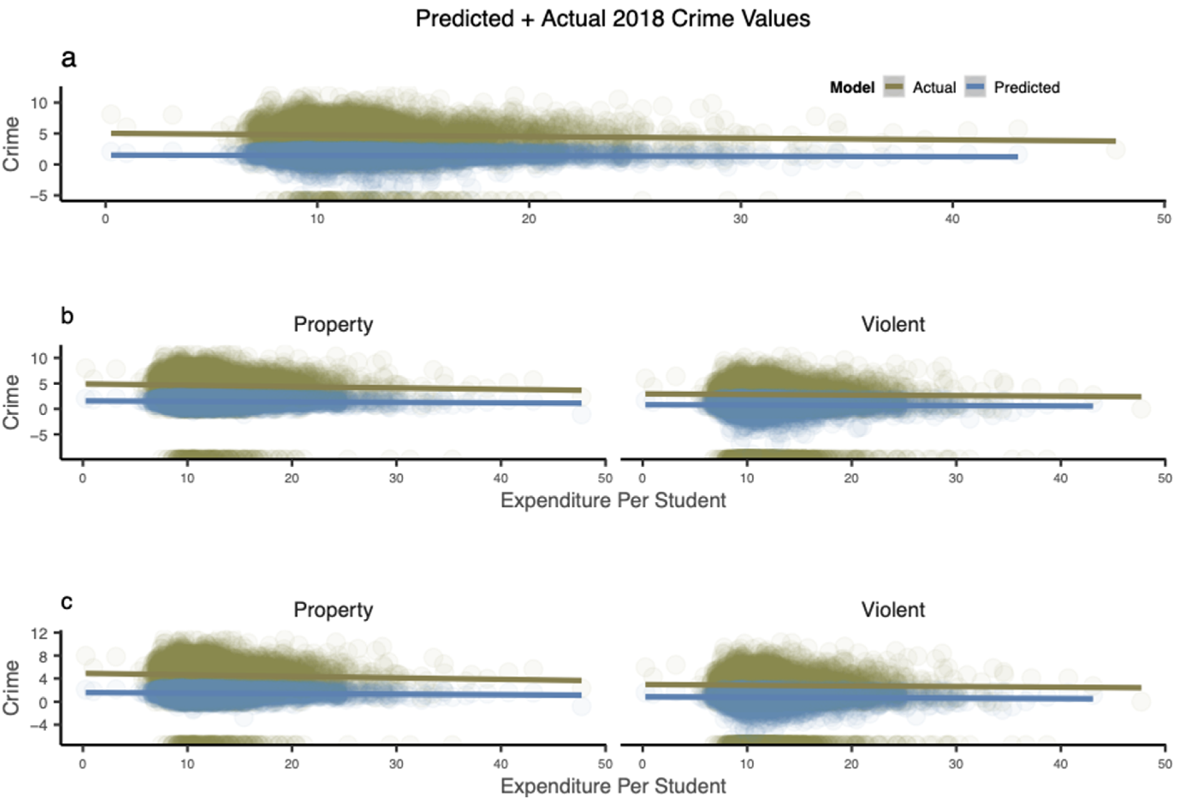
Using our 2018 holdout dataset, we established an RMSE of 0.077, a good fit. The predicted vs observed crime values are plotted in Figure 7a. We conclude that for every $1000 more a place spends on education, its total crime decreased by an average 2.19 ± 0.16 percent (1.89, 2.50).

4.2. Interaction of Education Spending on Crime Type (and Interactions among Other Variables)

In our second crime model, we looked at crime as a categorical variable of property and violent. Controlling for all other factors, we found that spending $1000 more per student on education engenders a significant decrease of 2.35 ± 0.16 percent in property crime (2.04, 2.66) and a non-significant decrease of 0.39 ± 0.24 in violent crime (−0.08, 0.85). In part, the non-significance of violent crime is explained by the interaction between year and crime: year to year, violent crime decreases much more slowly (an average decrease of 1.05 ± 0.14 percent per year (0.77, 1.33)), than property crime (an average of 3.20 ± 0.08 percent per year (3.03, 3.36)), shown in Figure 5b. In this model, with an interaction of education spending and crime type, we obtain an AIC of 351,520 and an RMSE of 0.17. One can see the effect size differences between total crime and crime type in Figure 5a,b.

After looking at several interactions (between covariates of per capita income and education spending and crime type), we found the interaction of per capita income and crime type to yield a 0.90 ± 0.14 percent decrease in property crime (CI: 0.62, 1.17) and a 5.25 ± 0.20 percent decrease in violent crime (CI: 4.85, 5.65); the interaction of education spending and crime yields a 0.85 ± 0.24 percent decrease for violent crime (CI: 0.39, 1.32), and a surprising 3.61 ± 0.16 percent decrease for property crime (CI: 3.31, 3.91). Thus, remarkably, what really seems to drive down property crime is an increase in education spending: a $1000 increase in education spending decreases property crime nearly four times as much as a 10 percent increase in per capita income. (Part of this might be explained by the fact that while income is not distributed equally, a place that has higher education spending might also have more services). A ten percent increase in student spending for a district with an expenditure of $10,000 (per student) would be $11,000. A ten percent increase in per capita income for a place of $40,000 would be $44,000. We can then add in content knowledge that the range in per capita income across places is roughly $310,000 and education spending is $40,000.

4.3. “Controlling” for Interactions among Property and Violent Crime

In a third crime model, we sought to test whether these findings would hold after accounting for possible differences in covariates among property and violent crime. For instance, as we see from Figure 7, per capita income and race covary, and thus, it seems that race would also vary as a function of crime. Though race wasn’t a specific focus of this paper, failing to account for the latent variance within a covariate could bias results. We built a third crime model similar to our first model; beginning with a base model (AIC: 346,408) including population and population density interacting with crime type, and then exchanged covariates in that interaction. We also reintroduced all variables removed from the first model. We added each covariate to the interaction part of the model by the order of its explained variance (seen in Figure 8a). Our third crime model AIC dropped to 332,541. The variables comprising our final model and their cumulative effects on AIC can be seen in Figure 8b.

Median income, some college, and law enforcement did not interact significantly with crime. However, using the likelihood ratio test, we determined that the inclusion of law enforcement was significant.

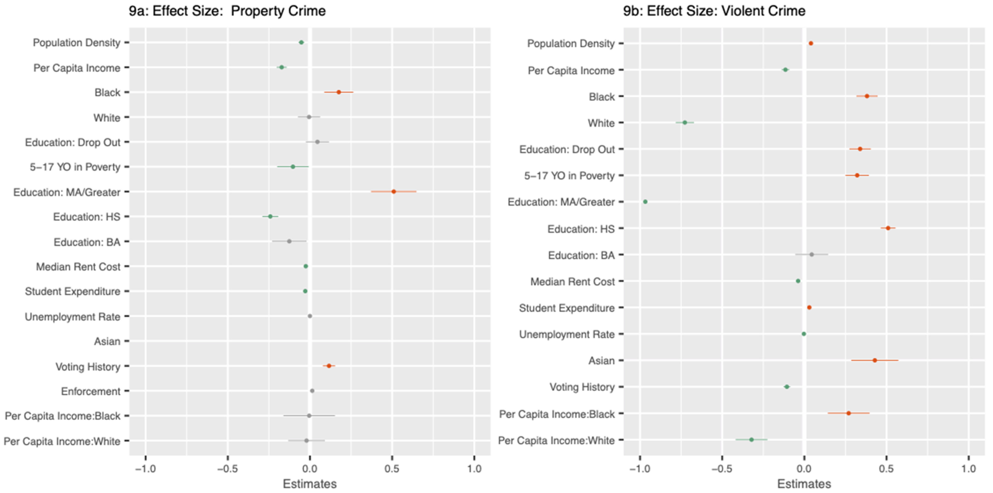
In this final, comprehensive model, conditioning on all variables seen in Figure 8b (including the interactions of per capita income and race), we conclude that a $1000 increase in education spending per pupil leads to an average 2.79 ± 0.16 percent decrease in property crime (2.49, 3.10) and a 0.21 ± 0.25 non-significant increase in violent crime (−0.27, 0.69). Regression coefficients for both violent and property crime interactions are shown in Figure 9a,b. We obtained an RMSE of 0.191, which is plotted in Figure 7c.

4.4. Other Measures of School Quality: Student Chronic Absenteeism, Teacher Absenteeism, and Teacher Retention

Additionally, we looked at several other proxies of school quality (shown in Figure 10) to better detect the existence of a causal factor, distanced from the correlation of education spending with other factors. In the interaction of student chronic absenteeism (more than 15 days missed per school year) on crime, we found that while property crime was significant and increased by 2.4 ± 0.75 percent for every 10 percentage-point increase in absenteeism, violent crime was not significant (1.9 ± 1.5 percent).

Next, we substituted teacher absenteeism for the education spending variable to determine whether teacher engagement might also explain crime rates. We found that a 10 percentage-point increase in teacher absenteeism correlated with a 1.1 ± 0.35 percent increase in property crime and a 1 ± 0.76 percent decrease in violent crime (importantly, if you do not look at the interaction of crime and teacher absenteeism, the effect is masked (0.05 ± 0.29 percent); again, emphasizing the need to break down crime into property and violent categories). There does not seem to be a logical hypothesis for how teacher absence would drive down violent crime, other than that it correlates with demographic factors (urban and low-income teaching can require more resources and be more taxing and thus, could drive teacher absenteeism).

One could make an argument for only including education spending in these models if it influences (directly or indirectly) the “school quality” variable (for instance, education spending could clearly impact variables like teacher salary or student to teacher ratio: either through paying teachers more, or by paying more teachers). However, we ultimately decided to include one model with all variables (chronic absenteeism, teacher absenteeism, and education spending) to see whether these other school quality measures explain variance that would otherwise be explained by education spending, establishing avenues of mediation for future consideration. Education spending continues to be significant, correlating with an on average property crime decrease of 1.98 ± 0.33 and a violent crime decrease of 0.60 ± 0.53. If we only look at a model including chronic absenteeism and education spending (without teacher absenteeism) there is a property crime decrease of 1.78 ± 0.33 and a violent crime decrease of 0.52 ± 0.27. This is in comparison with the corresponding model without these variables with a 2.35 ± 0.16 percent in property crime and a non-significant decrease of 0.39 ± 0.24 in violent crime. It is odd that education spending has a higher coefficient in a model with all three variables, then a model with only chronic absenteeism and education spending. More work must be done here to explore a possible interaction.

4.5. Lagging Data to Look at Spending and Absenteeism

In their paper, “Age and Crime”, Rocque and Chad (2015) write that “the relationship between age and crime is one of the most robust relationships in all of criminology”. Crime increases in early adolescence (around age 14) and then peaks in the early to mid 20s, declining thereafter. Thus, if chronic student absenteeism had an effect beyond incapacitation (missing of instruction), it should hold that if we lagged the data by five years, we should see an increase in crime (since those leaving high school would be at the end of this phase (age 23–24) and those in middle school would be entering into this phase). While lagging has no effect on property crime, a 10 percentage-point increase in chronic absenteeism correlates with a 4 ± 0.66 percent increase in violent crime.

The same concept should also hold for education spending and for teacher absenteeism. Interestingly, while education spending correlates with an increase in violent crime (0.63 ± 0.17 percent), it correlates with a reduction in property crime 2.41 ± 0.16. Interestingly, the effect of absenteeism on violent crime seems distinct from that of education spending on property crime, suggesting separate mechanisms through which these categories of crime can be targeted. In lagging the data, we found no effect of teacher absenteeism on either property or violent crime.

4.6. Range in Education Spending on Crime

Next, we looked at the effect of range in education spending (i.e., difference between the minimum and maximum education spending) on crime. A total of 2134 places will have access to more than one district. Where New York Department of Education will serve five separate counties comprising New York City; other cities or towns are served by multiple districts. In this case, when a town/city is served by multiple districts, there exists an inherent range: one district spends more than another. Here, we find no effect. (One caveat is that there was no way to locate the weights of the number of students attending each district). However, when we looked at the interaction of property and violent crime on education spending, we found interesting and significant effects. For every $1000 difference among districts (within a town/city), its property crime increased by an average 3.11 ± 0.35 percent (2.43, 3.80). Interestingly though, on average, its violent crime decreased by 3.05 ± 0.62 percent (1.83, 4.28).

Finally, we modeled range in education spending among counties: for crime type, every $1000 disparity in spending within a county is associated with an average 4.25 ± 0.57 percent (3.14, 5.37) decrease in total crime. In modeling the interaction of the range on property and violent crime, we found an average decrease of 3.61 ± 0.49 in property crime (2.65, 4.58) and a 2.48 ± 0.91 percent (0.70, 4.25) decrease in violent crime.

5. Discussion

We modeled education spending and crime in six separate models. Our first three models looked at total crime and property/violent crime as a function of education spending. Then we looked at lagged spending and education quality variables. Our final two models looked at how crime and crime type vary as a function of the range in education spending. The models adamantly demonstrate the inadequacy of modeling crime without distinct categories (property and violent), where important effects might otherwise be masked. In modeling the interaction between crime type and education spending, we found that education spending was associated with a 2.35 ± 0.16 percent decrease in property crime and a non-significant decrease in violent crime. There are several possible reasons for a non-significant effect of violent crime. First, as previously stated, on average over time, violent crime decreases much less than property crime. Second, as Jacob and Lefgren (2003) and Luallen (2006) note, schooling can concentrate young people, increasing criminal activity; thus, any positive effect of education spending on violent crime might be negated by this concentration effect. Still, it would be nice to know whether these effects are seen among all youth and how this varies as a function of urban populations and by wealth and economic disparities. We found that chronic absenteeism had a non-significant effect on violent crime; thus, this does not, of itself, support the findings by Jacob and Lefgren as well as Luallen, though one would expect that places of increasing absenteeism also correlate highly with other important factors (income, education attainment, etc.). Yet when we lag absenteeism by five years, conditioning on other important factors, we find an astonishing 4% increase in violent crime. This suggests a distinct mechanism by which education decreases violent crime (by a process other than those included in the model (attainment, wealth, employment). Oddly, we find no effect lagging absenteeism on property crime. This adds to the previous finding regarding violent crime because it is not merely that those with increased rates of absence are driven to criminality through poverty, else we would see similar increases in property crime. Beyond the incapacitation effect, other studies do demonstrate an effect of attendance. For instance, between 1999 and 2002, England piloted a program in which subsidies of up to £40 (with bonuses for course completion) per week were provided for low-income 16 to 18-year-old youths to incentivize school attendance and found that this program produced results slightly below a 5.5% reduction in property crime (Sabates and Feinstein 2008; Lochner 2020). Interestingly, Deming (2011), employs a different proxy of school quality, looking at public school choice lotteries (what number picked school students received) in the Charlotte-Mecklenberg school district and concluded that crime-reduction effects were concentrated among high-risk youth. Similarly, Cullen et al. (2006) found that for students who won their lottery to high-achieving schools compared with those who did not, self-reported arrest rates dropped by nearly 60 percent (3.8 percent versus 8.9 percent). (Self-reported arrest rates were corroborated by administrative data on incarceration rates for students in the sample). They conclude that the greatest reductions in crime were observed among the students whose peer quality is most likely to improve.

Wanting to home in on the specific causes of our findings and distinguish between education spending and wealth, we further modeled the interaction of per capita income and crime. We found that per capita income explained a large amount of variation in violent crime and a much smaller variation in property crime. On the other hand, controlling for this per capita income–crime interaction, we found that education spending singularly accounted for variance in property crime (driving down property crime nearly 4 times the amount as a 10% increase in per capita income. (It is also possible that per capita income effects on crime might be stifled by another finding that increases in wealth disparity significantly correlate with increases in property crime). Sabates (2008) found that reductions in poverty were associated with decreased conviction rates for violent crimes and drug-related offenses. Interestingly, looking at Figure 8b, one can discern discrete steps in AIC decrease–subsequent variables explaining distinct variance from preceding variables. For instance, despite being the 10th variable added to our third model, education explains a drastic and different variance: dropping the AIC from 334,022 to 333,011. Additionally, per capita income no longer correlated positively with property crime, a reversal that we traced to the interaction of the percent white constituents “race” variable on crime type.

Additionally, one would assume that if education spending plays an important role in decreasing crime so too would one’s level of education. Indeed, in our third and most comprehensive model we found that for every ten-percentage point increase in those who do not graduate high school, those who obtain a high school diploma, and those who obtain a master’s or greater, on average violent crime increases by 4.72 ± 0.72% and 3.04 ± 0.49%, and then decreases by 3.65 ± 1.42%. For the same increase in those who graduate high school, property crime decreases by an average 2.17 ± 0.25%; for those who obtain a master’s, it increases by 6.66 ± 0.73%. Poorer, less educated people experience more violent crime; wealthier, more educated people experience more property crime. Results from Lochner (2004) suggest that completion of the twelfth grade causes the greatest drop in incarceration and that there is little effect of schooling beyond high school. Machin et al. (2011) supports this finding: men who finished high school (between the ages of twenty-one and twenty-five) were eight times less likely to be arrested than those who had dropped out. Sabates (2008) found that increases in educational attainment was associated with decreases in conviction rates for most offenses (burglary, theft, criminal damage, and drug-related offenses) but not for violent crime.

Additionally, we regressed the range in education spending on total crime and crime type to see whether disparities in educational spending had significant effects above and beyond per capita income and whether accounting for this specific variance altered effects of other important variables. While we expected that crime might increase with whatever latent or non-latent construct pushes the presumed inequity, we were surprised by the interaction of range on crime type. It is possible that property crime increases among cities/towns because the extremes of wealth motivate more minor thefts, while violent crimes decrease because the increased affluence deflects the factors begetting violence. Essentially, we wonder whether violent crime happens at home (in poorer neighborhoods) while property crime happens elsewhere (in wealthier areas). Supporting this hypothesis, Immergluck and Smith (2006) found that higher foreclosure levels do contribute to higher levels of violent—but not property—crime (2.8 foreclosures per 100 corresponds to neighborhood increase of 6.7% violent crime), distinguishing not only factors that impel violent vs property crime but also, to some extent, their origins.

There has been a good deal of research looking at income inequality and increased rates of criminality, particularly with those crimes involving monetary gain. Some studies demonstrate little effect (Allen 1996; Bourguignon 2002; Neumayer 2005). In one study of municipalities in Sao Paulo, Brazil, Scorzafave and Soares (2009), find the elasticity of pecuniary crimes relative to inequality to be 1.46. Zhang (1997) demonstrates an elasticity of property crimes in relation to the Gini Index of 1.65. Our study supports these results: specifically, that property crime increases with wealth disparity. For every $1000 increase in spending disparity, property crime increases (4.10 ± 0.34%). However, while some studies (Kelly 2000; Fajnzylber et al. 2002; Choe 2008) find increased violence with wealth disparity, we found the contrary: that violent crime decreased (3.06 ± 0.61%). While Bourguignon (2002) studied overall crime rate, our research suggests that crime rate should be broken into property and violent categories. While Chloe looked at states to measure crime and disparity: we looked at towns and cities to measure these. Our study emphasizes the need to both break crime into separate categories and to research it at smaller levels (ideally at the level of neighborhood). A notable example of this is the fact that while we observed a decrease in both violent and property crime among counties as range in spending increased, it might be that we could have seen the same property crime increases as we found among cities/towns, but for the fact that population density decreases as we move from place to county.

There are several interesting and unexpected findings ancillary to education spending that should be discussed. (1) We found no significant effect of unemployment. One can see from Figure 2a that the comparative variance explained by unemployment is minimal; the only variable explaining less variance is whether someone graduated from high school. Second, ACS estimates in smaller areas are collected over a 5-yr period and averaged, which would fail to capture extreme yearly behavior like the market crash of 2008. Our finding conflicts with some research and both the economic theory of crime proposed by Becker (1968) viewing crime as a type of work requiring time and yielding economic benefits (those without work would have more time and more to gain though this is not reflected in the data), and it also conflicts with the idea of incapacitation (those occupied will not otherwise commit crimes). Raphael and Winter-Ebmer (2001) conducted a panel-analysis from 1971–1997 to look at state levels of unemployment and crime and determined significant positive effects of unemployment on property crime rates, though weaker evidence for violent crime rates. For reasons we have emphasized in this paper, looking at the state level is problematic. While it decreases uncertainty in estimates (in this case, unemployment), it also does not adequately acknowledge differences within a state. From a policy perspective, it does nothing to inform states whether, where, and how much to invest in specific places to stem crime. Edmark (2005) employed a Swedish dataset from 1988–1999 and used a fixed-effects model including time and county-specific effects to find that unemployment had a positive, significant effect on some property crimes (burglary and bike and car theft). This work did not go below the level of county. Future work should focus on the relationship between unemployment and crime at the neighborhood level.

(2) Notably, while funding for law enforcement has grown at a rate 25% greater than that of education, we found that for every ten percent increase in officers, crime actually increased by an average 0.11 ± 0.02%. Perhaps more importantly, in none of the above models did law enforcement correlate meaningfully with crime when conditioning on other factors. While there have been papers published regarding effects of law enforcement on crime, much of it seems to be theory based. Worrall (2008) published a paper looking at the Local Law Enforcement Block Grants (LLEBG) Program, investing $3 billion to local jurisdictions to reduce crime. He conducts a panel analysis from more than 5000 cities over a 12-year period (1990–2001) and regressed crime rates on funding and other demographic controls. Interestingly and importantly, the author found that LLEBG drove significant reductions in serious crime; however, the results revealed that this decrease did not occur through the hiring of additional officers, which comports with our work. Additionally, through the data, the author could not conclude what these crime reduction mechanisms were.

Certainly, other factors affect crime and its reporting. The political climate, which we accounted for as voting history, (though we could not locate data below the county level) and direction of the district attorney (not accounted for in our models) impacts whether law enforcement deems something a “crime” and whether an arrest is made. It is also important to note that just because a crime is not reported does not mean that a crime did not occur. The United States Department of Justice (2019c) publishes a dataset through the National Crime Victimization Survey (NCVS), aiming to reconcile—through representative samples based on residential addresses—neighborhood disparities in crime reporting. Though there are 17,985 police agencies in the 3131 counties and 36,000 distinct places (townships, towns, cities), the departments providing crime data to the FBI are far less—in any given year it ranges from 8500 to 9500. Fortunately, the trend to report crime data is upward.

Future work should incorporate data from the NCVS in addition to the UCR datasets and discrepancies between datasets. Follow-up analyses should also include defining an exogenous variable or propensity scores approach to further determine causality. Additionally, further work must be done to get below the level of city/town down to neighborhood. Other avenues would include further controlling for factors that distinguish school district quality from district spending; looking at whether the specific allocation of money within districts or spending in specific areas—instructional spending, for instance—has an effect beyond “total current spending”; and whether there exists an expenditure threshold, where up to a certain point crime declines more quickly (possibly as a function of the proportion of children living in poverty). Similarly, further work should account for incarceration rates alongside school spending as research demonstrates crime-reducing effects of incarceration (Western 2006; Levitt 2004; DeFina and Arvanites 2002). Lastly, one could consider looking at crimes not merely by where they occurred but by where the people who committed them reside: such research would provide a more nuanced understanding of the various shifts and interactions among levels of crime and how the effect sizes of those interactions might vary as a function of assailant’s proximity to the location of the crime. Again, the work of Chetty et al. (2018), mentioned in the introduction, demonstrates the importance of looking at demographic patterns on a fine-grained level.

As Burtless (1999) writes in his paper, Effects of Growing Wage Disparities and Changing Family, U.S. income inequality soared after 1979 and by 1993 it reached a peak unseen since the conclusion of the Great Depression. The following year, 1994, Congress passed the Crime Bill, allocating 9.7 billion dollars in funding to Prisons and the addition of 100,000 officers. 27 years after passing that bill, the US prison population has more than doubled. On the other hand, education spending among youth seems to have received the bad end of a hyper-polarized stick. Our research adds to the growing body of work on education and crime, demonstrating that education spending does matter, and that its politicization can literally be dangerous.