Article

Indoor/Outdoor Environmental Parameters and Window-Opening Behavior: A Structural Equation Modeling Analysis

1
Department of Civil and Environmental Engineering, University of Washington, Campus Box 352700, Seattle, WA 98195, USA
2
Department of Industrial and Systems Engineering, University of Washington, Campus Box 352650, Seattle, WA 98195, USA
*
Author to whom correspondence should be addressed.
Buildings 2019, 9(4), 94; https://doi.org/10.3390/buildings9040094
Submission received: 21 February 2019 / Revised: 16 April 2019 / Accepted: 17 April 2019 / Published: 20 April 2019

Abstract

:
In moderate climates, the operation of windows is the most common way to control for thermal comfort. Window-opening behavior (WOB) is a complex process influenced by multiple factors, yet only simple bi-variate analyses between variables obtained from longitudinal datasets have been examined. The goal of this study is to investigate the effects of indoor and outdoor environmental parameters on WOB using a statistical modeling approach called “structural equation modeling.” The results show that the indoor environmental parameters, such as operative temperature and air velocity, mediated the relationship between the outdoor environmental parameters, such as outdoor air temperature and wind gust, and the WOB. The indoor wet-bulb globe temperature rose as the solar radiation increased, and subsequently, both parameters affected the WOB. Also, an increase in outdoor wind gust led to higher indoor air velocity, which in turn resulted in a lower chance of occupants opening the window. By enhancing our understanding of the relationship between these theoretical parameters, improved design strategies on the mediating parameters can be prioritized and communicated early in the building design phase leading to more informed design decisions.

1. Introduction

Successful energy efficient design strategies require the adoption of advanced building system control technology but also a better understanding of how occupants engage with that system. This is because previous studies have demonstrated that greater personal control over their microenvironment can lead to an increase in indoor satisfaction and comfort [1] even in a wider range of conditions. Occupant behavior may include opening and closing windows or blinds, overriding or deactivating energy-saving strategies, plugging in small devices, changing the cooling or heating setpoints, and use of lights which in combination will affect the total amount of energy used in the building. These individual occupants’ preference and the choices they make in the building has changed the way industry provide building design and operational services. When possible, building owners seek more climate-responsive designs allowing for more personal control and interaction which has demonstrated significant energy savings as compared to fully mechanically operated buildings [2,3]. A study by Wang and Greenberg [4] using building performance simulation tool demonstrated that mix-mode ventilation strategy taking into consideration of window operations resulted in 17–47% of energy savings.
These climate-responsive designs are particularly favorable in moderate climates. In moderate climates, the operation of windows is the most common way to control for thermal comfort [5]. Window operation is a complex process influenced by multiple factors [6] and is important to understand for many reasons. Window operation is associated with ventilation, indoor air quality, and energy consumption [5,7]. Further knowledge of the mediating effect of indoor environmental parameters on the relationship between outdoor environmental parameters and window operation in these interactive window systems can aid in refining the simulation models for predicting energy use. Increased understanding of window operation behavior and motivation will also allow architects and engineers to improve building envelope and mechanical strategies to optimize the operation of buildings given the growing interaction between its occupants and building systems. Specifically, this paper extends other occupant behavior theory related to comfort driven adaptive WOB by investigating latent variables and mediating effect of indoor environmental parameters on the relationship between outdoor environmental parameters and WOB in a naturally ventilated building.
Previous studies demonstrate the large discrepancies found between simulated and measured energy consumption in buildings due to occupant behavior [8,9]. Van Raaij and Verhallen [8] found that energy uses of various pattern groups differed considerably, up to 31% in buildings through field studies. Karlsson et al. [9] found that actual measurements of energy use differed up to 50% as compared to predicted and simulated energy use for low-energy residential buildings.
In terms of WOB, Fabi et al. [6] organized the influencing drivers from existing studies into five groups: physical environmental factors, contextual factors, psychological factors, physiological factors, and social factors. While they found that most of the recent studies on window operations focused on outdoor and/or indoor temperatures among other environmental factors, they also highlighted many drivers and motivational factors for engaging in such behavior. For example, they found that interactions of the users with the building control (windows or heating set-point) are not only influenced by perceived thermal conditions but also by the response to perceived indoor air quality, draft, rain, outdoor noise levels, and the desire to conserve energy. These motivations tend to co-vary in naturally ventilated buildings, and even as indoor temperature produces the discomfort that triggers window opening, the acceptability of an open window will be determined by the conditions outside. Their analysis also found that there is no conclusive set of driving forces suggesting a relational model between these variables. No single model could best fit or predict the WOB, and associated energy use as these studies were conducted in different building types (e.g., offices versus residential), occupancy (e.g., single versus double occupancies), countries with different cultures (North America versus Europe), climate, and length of observation periods (e.g., seasonal versus full or multiple years).
Nevertheless, some parameters were found to be consistently associated with WOB [6]. For example, different correlations and dependencies were established in many studies [10,11,12,13,14,15,16] between outdoor temperature, indoor temperature, occupancy, the season of the year, time of day, previous window state, wind speed, and solar radiation. Several studies [5,12,13,16,17,18,19,20] conducted in office buildings suggested that outdoor air temperature was the dominating driver for occupants’ WOB. This is consistent with early studies on this topic, such as [11,21]. Other studies [5,12,17,19,20] found that both outdoor and indoor air temperature contribute to WOB. For example, Rijal et al. [22] investigated window opening behavior in residential buildings in 140 Japanese homes over a four-year period. They found a higher likelihood of opening windows in free-running buildings and the opening correlated highly with outdoor and indoor air temperature. Some authors [14,15,23] indicated that indoor temperature is more predictive of WOB while others [11,13,16,18,21] found that outdoor temperature is still the dominating driver of the two. This disagreement among researchers was echoed in a literature review by Stazi et al. [24]. Additional environmental factors were similarly considered in previous studies. Landsman et al. [25] developed a window opening model for a building using natural night ventilation and the results showed that window opening behavior was most dependent on indoor air temperature and mass temperature. Pan et al. [19] assessed the effect of outdoor relative humidity, solar radiation, and wind speed. While these factors indicated a significant impact to the WOB, indoor and outdoor temperatures had a greater impact on the WOB. Andersen et al. [26] conducted similar studies in residential buildings and determined that the indoor CO 2 level was the most important factor for predicting window openings as opposed to indoor or outdoor temperature. Besides environmental factors, contextual drivers have also been studied. Belafi et al. [27] developed a window opening model for schools using surveys and measurements. Contextual (single teacher and rotating teachers) and social behavioral aspects (opening/not opening based on student complaints) appeared to influence window opening behaviors.
Logistic regression remains a popular method among researchers for modeling WOB [5,16,18,19,28,29]. However, other modeling approaches have also been used in the literature. Haldi and Robinson [12] proposed a hybrid of techniques including logistic regression, Markov chains, and continuous-time random processes. Pan et al. [30] focused on an improved model based on Gauss distribution, which showed higher prediction accuracy over logistic regression model. Markovic et al. [31] applied deep learning methods in window opening model, which showed significant improvement in modeling imbalanced properties of window states, where the proportion of closed windows was larger than opened.
It can be argued that the indoor environment is affected greatly by the outdoor environment, especially for naturally ventilated buildings during non-heating seasons. This is also the basis for the adaptive thermal comfort model used by the American Society of Heating, Refrigerating and Air-Conditioning Engineers (ASHRAE) Standard 55 [32] and discussed in detail by Nicol and Humphreys [14]. Although the indoor environment may appear to be related to occupants’ thermal sensations in a more direct sense, it should be noted that indoor variables such as temperature, relative humidity, air velocity can largely depend on the outdoor climate, which indicates that the indoor variables cannot serve as independent predictors without considering the outdoor variables. On the other hand, models only considering outdoor variables would fail to reflect each building’s uniqueness in terms of its design, location, and functionality.
The goal of this study is to examine the relationships among indoor/outdoor environmental parameters and WOB using structural equation modeling (SEM). SEM is a technique described as “a second generation of multivariate analysis” that provides multiple relationships among variables [33]. In SEM, relationships among more than one predictors and response variables are estimated simultaneously. This is especially distinguished from bivariate correlations where only two variables can be investigated. Due to SEM’s ability to generate structures among variables, SEM can reveal direct as well as indirect effects [34,35]. Such indirect effects can be determined by testing if any mediating effects exist and if the mediating effect is full or partial. Figure 1 shows the graphical illustration of a mediation model with mediator variable M, independent variable X and dependent variable Y. The direct effect is represented by c on the casual relationship between X and Y, whereas the indirect effect is represented by the product of a and b. Given significant indirect effect, the mediator M fully mediates the relationship between X and Y if no significant relationship between X and Y is found. Given significant indirect effect, if the relationship between X and Y is also significant, M partially mediates the relationship between X and Y.
It is noted that previous studies investigating WOB in experimental settings were often based on longitudinal datasets analyzed using multivariate analyses and did not explicitly discuss the mediating role of indoor environmental parameters on WOB. While regression analyses reveal relationships among variables, they do not imply that the relationship is causal. In this study, structural equation modeling is applied to examine the causal chain of the effect of indoor/outdoor environmental parameters on WOB using the ‘sem’ package [37] in R [38] that is based on the reticular action model (RAM) formulation [39].

2. Materials and Methods

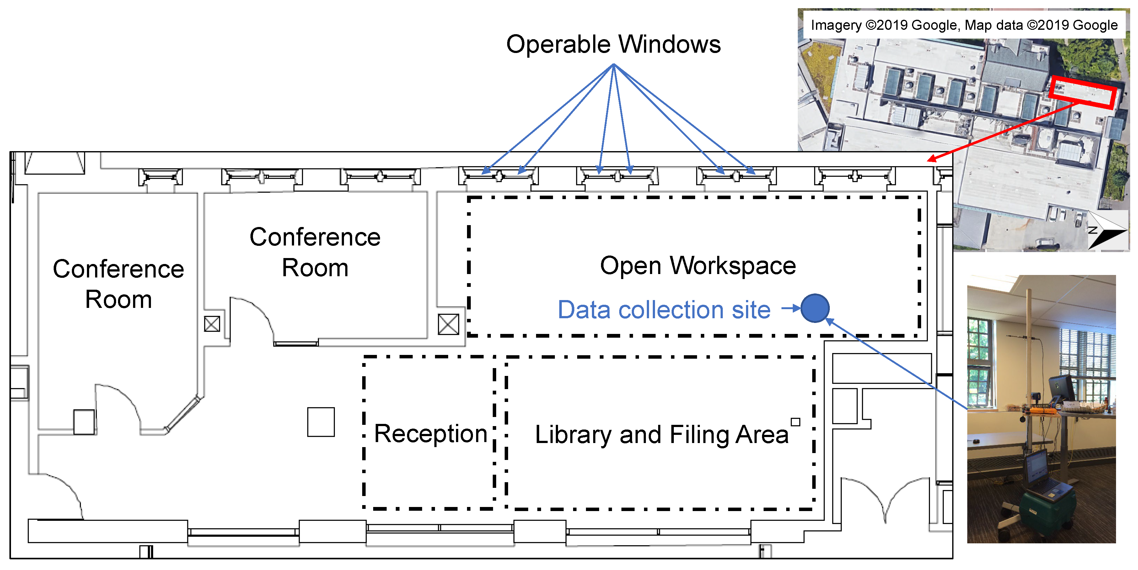
2.1. Case Study Building

The indoor environment data were collected daily from July 2014 through March 2015 in an office room on the third floor of the Husky Union Building (HUB) on the University of Washington campus. The office was located around the perimeter of the building, which had a central three-story atrium with a large staircase. The office was approximately 125 square meters in area with six west facing operable windows and regularly occupied by four to six staff members. According to the staff, the office was usually occupied on weekdays from 8 a.m. to 8 p.m. The staff included a full-time supervisor and several part-time student employees with flexible schedules. Therefore, the occupancy of the office varied from day to day. However, the number of people in the office area did not vary significantly during the hours of 8 a.m. to 8 p.m.
Figure 2 shows the layout of the selected office. There were two conference rooms in the office. The main office area was divided into three sections: reception, library and filing, and the seated area where modular workstations were located. The office was on the third floor with west-facing, operable windows. Six of the operable windows were adjacent to the seated area, and the occupants recorded their openings. The total area of the windows in this office was approximately 9.5 m 2 , which equated to a window-to-floor area ratio of 7.6%. All of the measurements and observations were collected from the occupant seated area. Typically, three to four student employees were working in the office during the day with a staff supervisor. Because services were provided mostly by appointment, the office staff did not have fixed schedules, which made the equipment setup and data retrieval process challenging.

2.2. Indoor Environmental Data Collection

The data collection started in July 2014 and stopped at the end of March 2015. The recorded data were divided into three separate periods as shown below and seasons were defined by the calendar, i.e., equinoxes in the fall and solstices in the summer and winter.
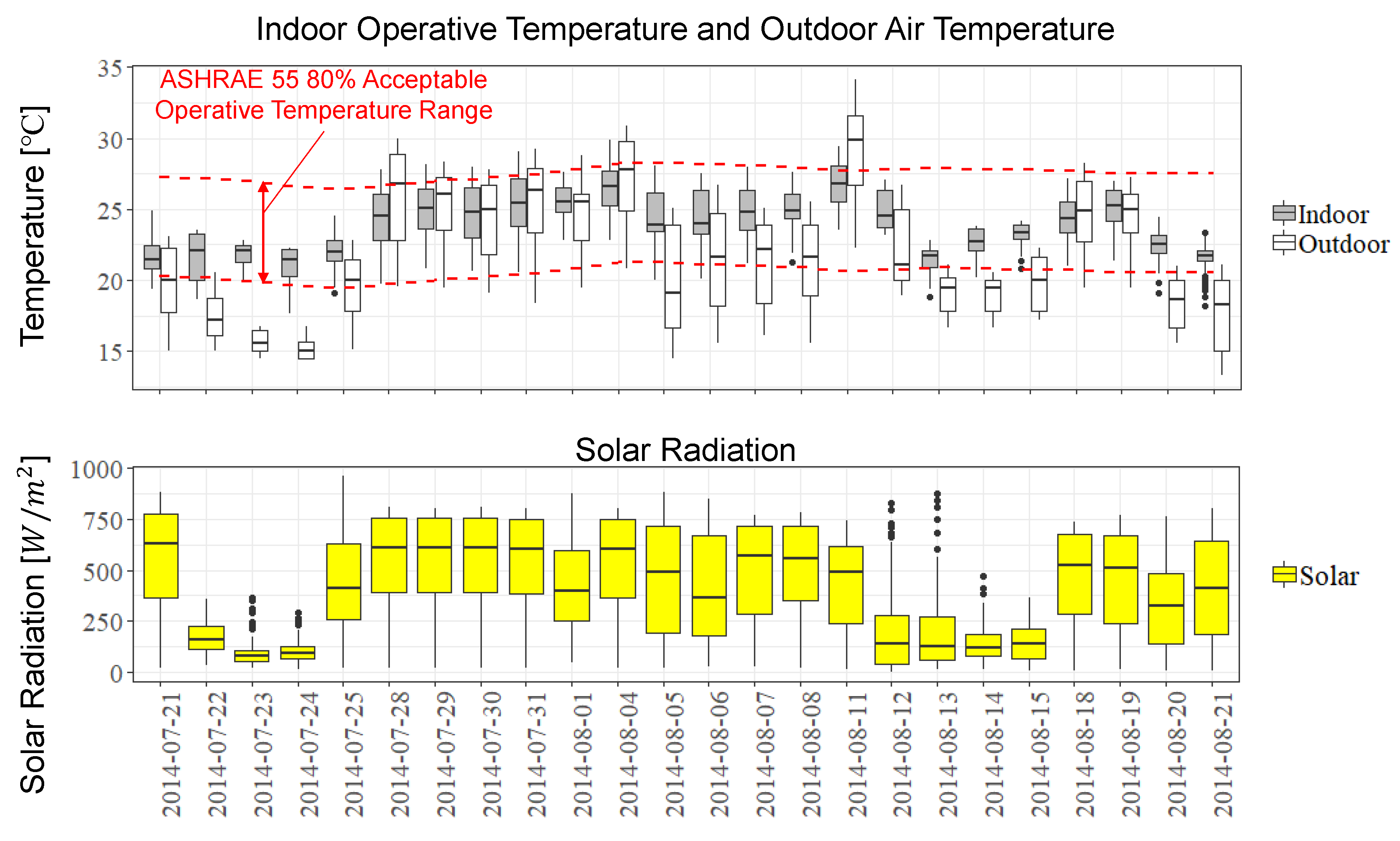
  • 12 July 2014–21 August 2014 → Summer
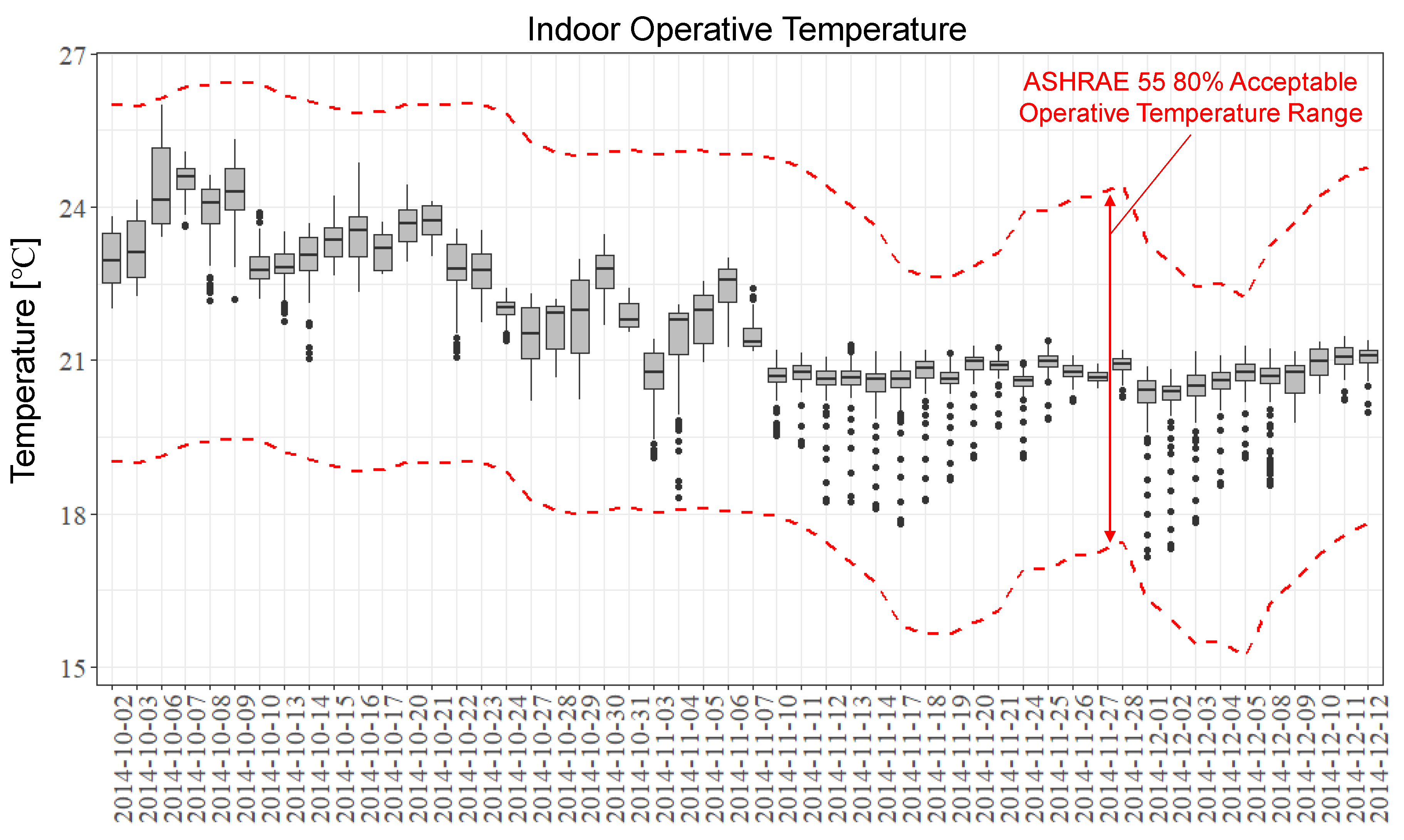
  • 2 October 2014–12 December 2014 → Fall
  • 6 January 2015–20 March 2014 → Winter
The authors consulted the ASHRAE Standard 55 [32] and Performance Measurement Protocols for Commercial Buildings [40] to determine the necessary equipment for evaluating the indoor environmental parameters of commercial office space (see Table 1). The ASHRAE Standard 55 [32] and Performance Measurement Protocols for Commercial Buildings [40] provided specific instructions regarding the measurement of indoor air temperature. The air temperature and air velocity sensor were placed at three different heights, i.e., 0.1 m, 0.6 m, and 1.1 m, and the measurements were used to calculate the spatial average air temperature for seated occupants. The globe temperature, CO 2 and relative humidity sensors were placed at the desk level. The sound meter was mounted between 1.1 m and 1.7 m above ground.
All items listed in Table 1 required annual calibration. Because they were purchased at the beginning of the study and calibrated by the manufacturer before delivery, the sensors were assumed to work according to specification during the study period. The sensors were assembled and mounted to an IV pole typically used in hospitals to create a data-gathering station. The data from the individual device were downloaded twice a week between the hours of 1 p.m. and 2 p.m. The timing and frequency of the data downloading were determined so that the interruptions of recording were minimized while the storage capacity of the devices was not exceeded. Loss of data for several hours occasionally happened due to malfunction. The downloaded data were stored locally on a designated laptop and organized by the date of retrieval.
Thermal comfort models in ASHRAE Standard 55 [32] required the use of operative temperature. In this study, the globe temperature was measured directly as an approximation of operative temperature. As shown in a study by Kazkaz and Pavelek [41], the difference between operative temperature and the globe temperature was within 1 °C in their experiments. The battery-powered globe temperature meter had limited recording capabilities and encountered numerous malfunctions, which resulted in more missing data compared to the other devices. In contrast, the air temperature meters were more reliable with minimal missing data. Linear regressions conducted using the globe temperature and indoor air temperature measurements for summer, fall and winter seasons separately showed that the two parameters were highly correlated with R 2 s greater than 93% for all three seasons. Therefore, the operative temperature used in this study was estimated based on the indoor air temperature measurements using the linear regression results to ensure minimal data loss. The linear regression results for the three seasons are summarized in Table 2.

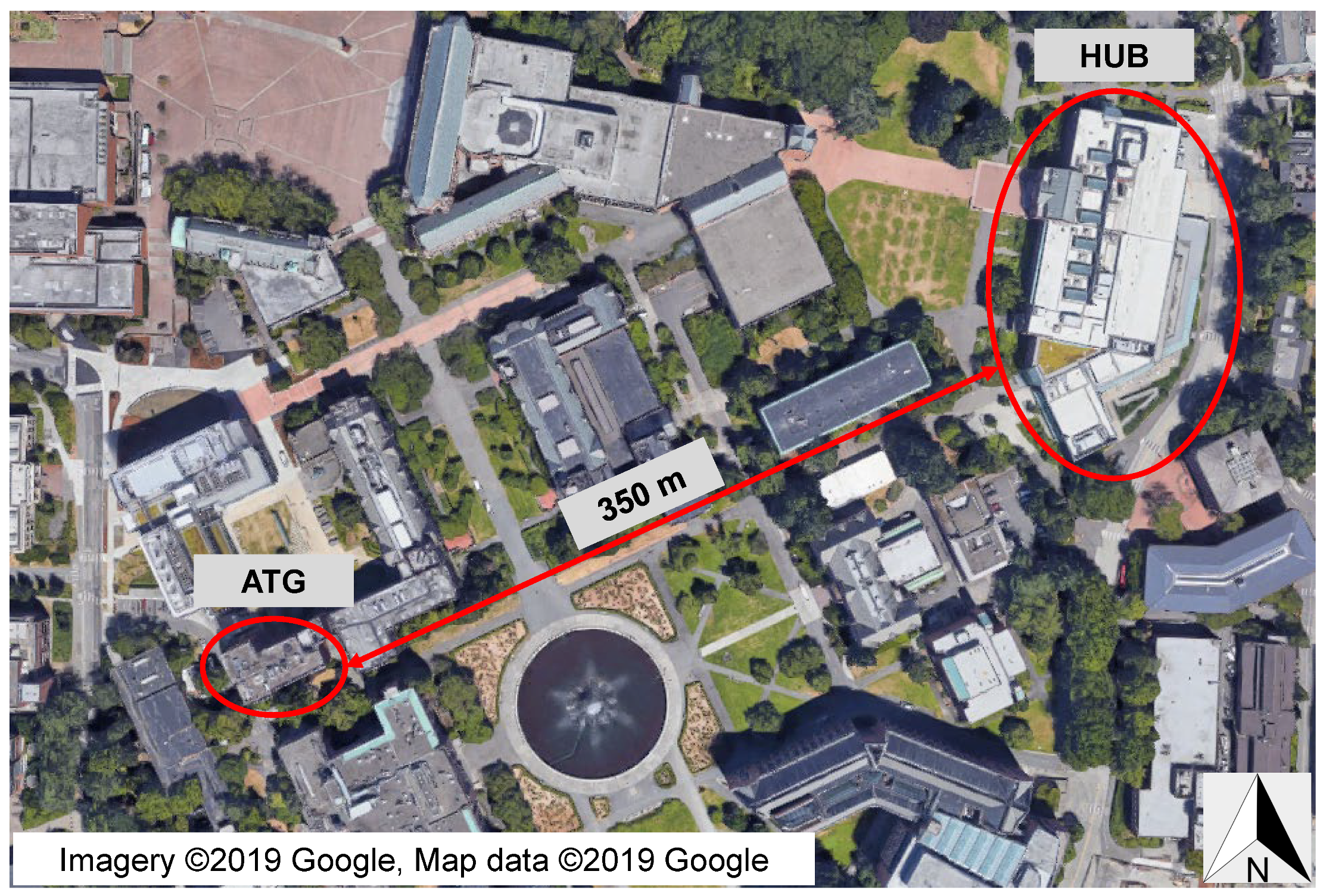
2.3. Outdoor Environmental Data Collection

The outdoor environmental data, such as air temperature, relative humidity, wind speed, wind gust, and solar radiation, were obtained from a weather station operated by the Department of Atmospheric Sciences at the University of Washington [42]. The weather station was located on the rooftop of the Atmospheric Sciences Building (ATG) approximately 350 m from the Husky Union Building (see Figure 3), which ensured that the outdoor weather observations were representative of the local climate.
The ATG weather station published 1-min observations each day [42] in UTC. The data of relevant days were downloaded, processed and merged with the indoor environmental data collected from the HUB. The outdoor air temperature was used to calculate the 80% acceptable operative temperature ranges following the ASHRAE Standard 55 [32]. The upper and lower limit of the 80% acceptable range is given in Equations (1) and (2). The variable t p m a ¯ was defined as the “prevailing mean outdoor air temperature” in ASHRAE Standard 55 [32], and was calculated based on the arithmetic average of the mean daily outdoor air temperatures over no fewer than 7 and no more than 30 sequential days prior to the day in question (a 7-day period was used in this study).
Upper 80 % acceptability limit   ( ° C ) = 0.31 t p m a ¯ + 21.3
Lower 80 % acceptability limit   ( ° C ) = 0.31 t p m a ¯ + 14.3

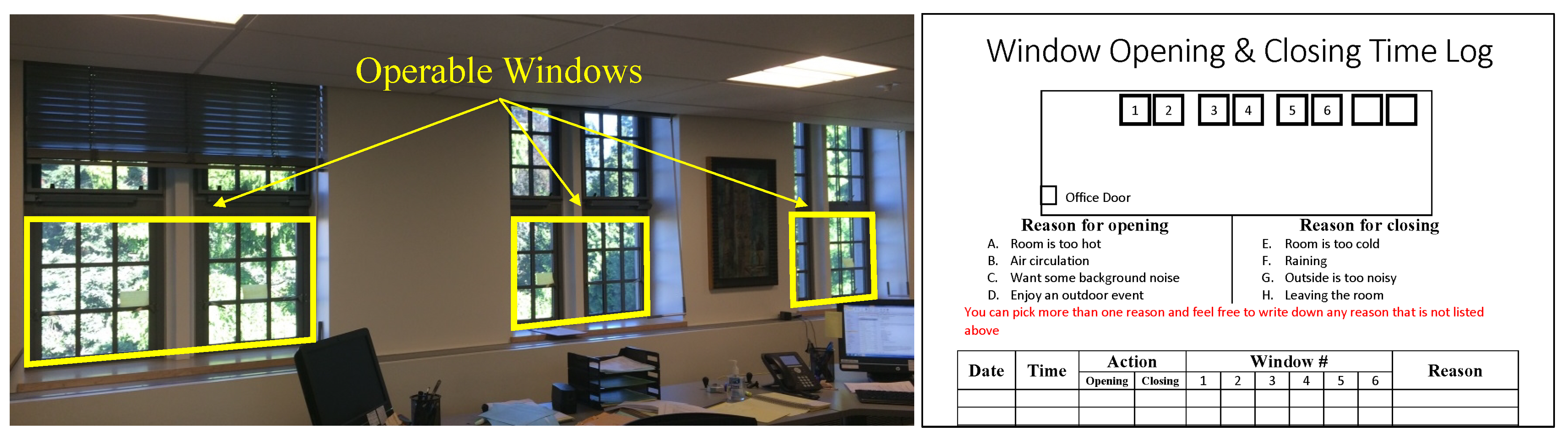
2.4. Occupant Monitoring

One important feature of the case study building was that it used natural ventilation for most of the spaces. The natural ventilation primarily depended on the computerized auto-controlled windows and exhaust fans to bring in outside air for ventilation [43]. Occupants were also expected to regulate the thermal comfort and air quality by using the manually operable windows. The mechanically assisted natural ventilation had three modes of operation: normal, heating, and night ventilation. Each mode operates under different sequences based on the continuous monitoring of space temperature and carbon dioxide levels, with the objective being to maintain comfortable space temperature and to keep carbon dioxide concentration at a designated level. The ventilation system was designed to maintain the temperature between 24 and 26 °C (76 and 78 °F) in normal mode and above 20 °C (68 °F) during the heating season. The carbon dioxide level was maintained below 800 ppm, assuming a 300 ppm outdoor reference [43]. The auto-controlled windows would open when the carbon dioxide level exceeds 800 ppm, and they were only installed in offices, conference rooms, and the atrium. Most offices either had upper auto-controlled windows and lower manual windows or were equipped solely with manual windows. For the case study office, the upper windows were controlled automatically by the building, while the lower ones were controlled manually by the occupants.
To thoroughly study the impact of indoor and outdoor environment on window opening and closing behavior in the office, the operation of both auto-controlled and manual windows was recorded. Openings and closings of the manual windows were recorded by occupants using a form designed by the authors as shown in Figure 4. Because the auto-controlled window operation was not recorded electronically, a laptop was used to take photos of the auto-controlled windows every 60 s to determine their status. The status was recorded as either open or closed. The angles of the openings were not measured.

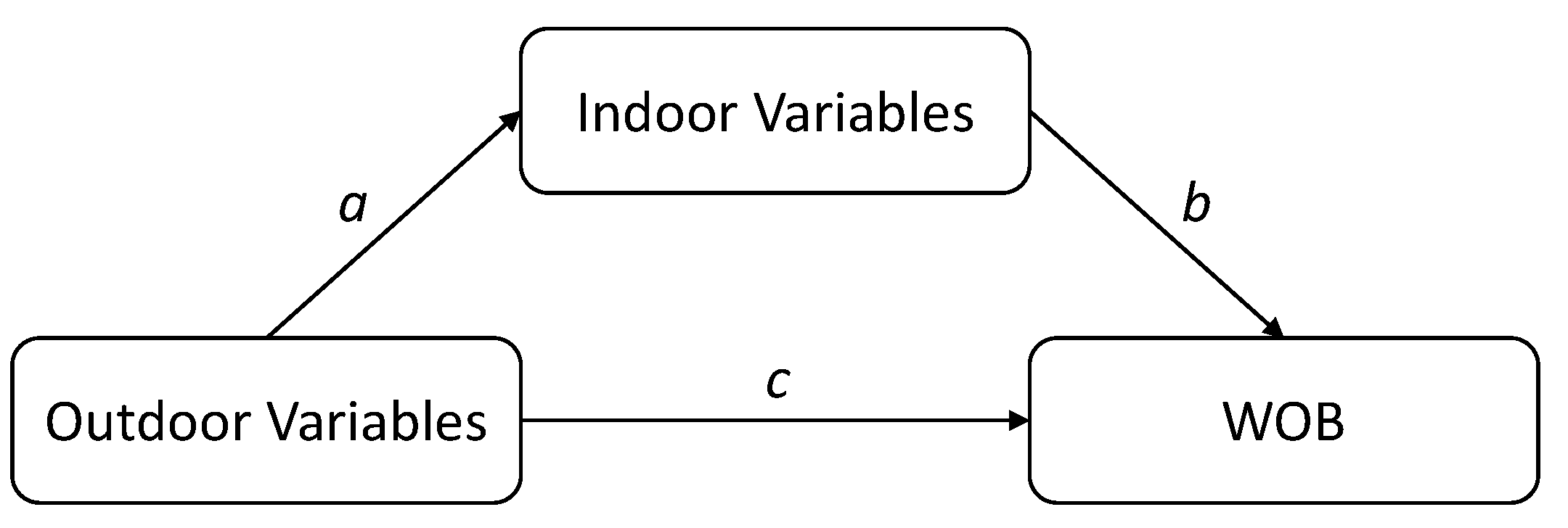
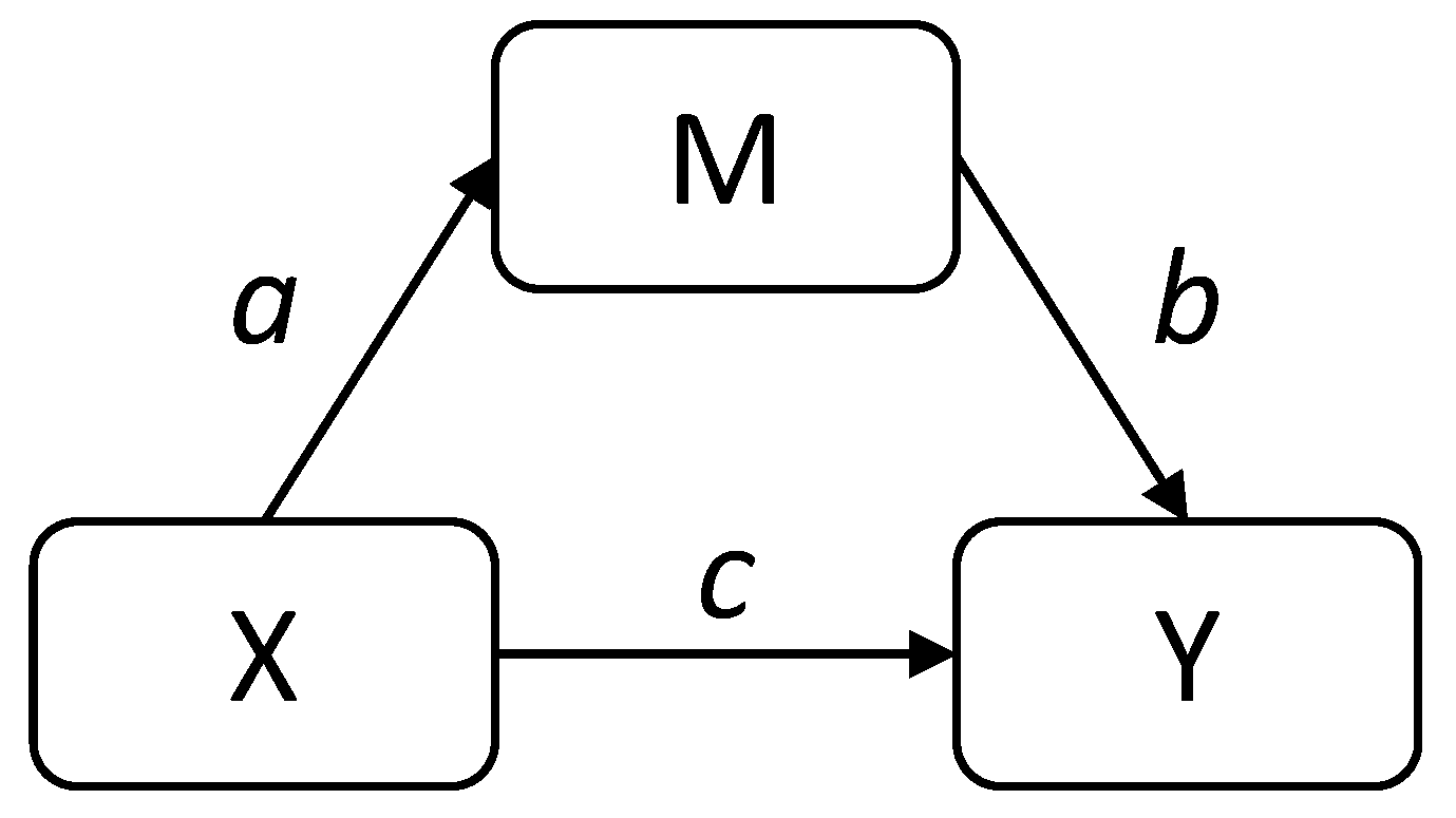
2.5. Structural Equation Modeling

SEM enables researchers to investigate multiple relationships among variables, including the mediating effect. By using SEM, the authors aimed to test how outdoor and indoor environmental parameters affected WOB. Eleven variables—Out_RH, Out_Temp, Out_WindDir, Out_WSpeed, Out_Gust, Out_Rad, Ave_Av, In_CO2, WBGT, Sound_dB, and WOB—were initially examined and found to be normally distributed at α = 0.05 (Kolmogorov-Smirnov test statistics are given in Table 3), except for Ave_Av. The data were then transformed using Z-standardization. Figure 5 illustrates the conceptual model of indoor variables’ mediating ability between outdoor variables and WOB. Specifically, outdoor environmental variables, including Out_RH, Out_Temp, Out_WindDir, Out_WSpeed, Out_Gust, and Out_Rad, were set as independent variables. The indoor environmental variables, including Ave_Av, In_CO2, WBGT, and Sound_dB, were used to test the mediating effect on the relationship between outdoor environmental variables and WOB. In Figure 5, the effect of outdoor variables (independent variables) on indoor variables (mediator) is represented by a; the effect of indoor variables on the WOB (dependent variable) is represented by b; the effect of outdoor variables on the WOB is represented by c. When a, b, and c are all significant, the indoor variables would partially mediate the relationship between outdoor variables and WOB. If only a and b are significant, the indoor variables would fully mediate the relationship between outdoor variables and WOB. The package ‘sem’ [37] in R [38] was used to test the structural equation model.

3. Results

3.1. Descriptive Statistics

The results of the data collection consisted of the time series of the parameters listed in Table 3 (refer to the Abbreviations section for descriptions of each parameter). These parameters were recorded at one-minute intervals daily and were compared with the ASHRAE 55 comfort standard [32].

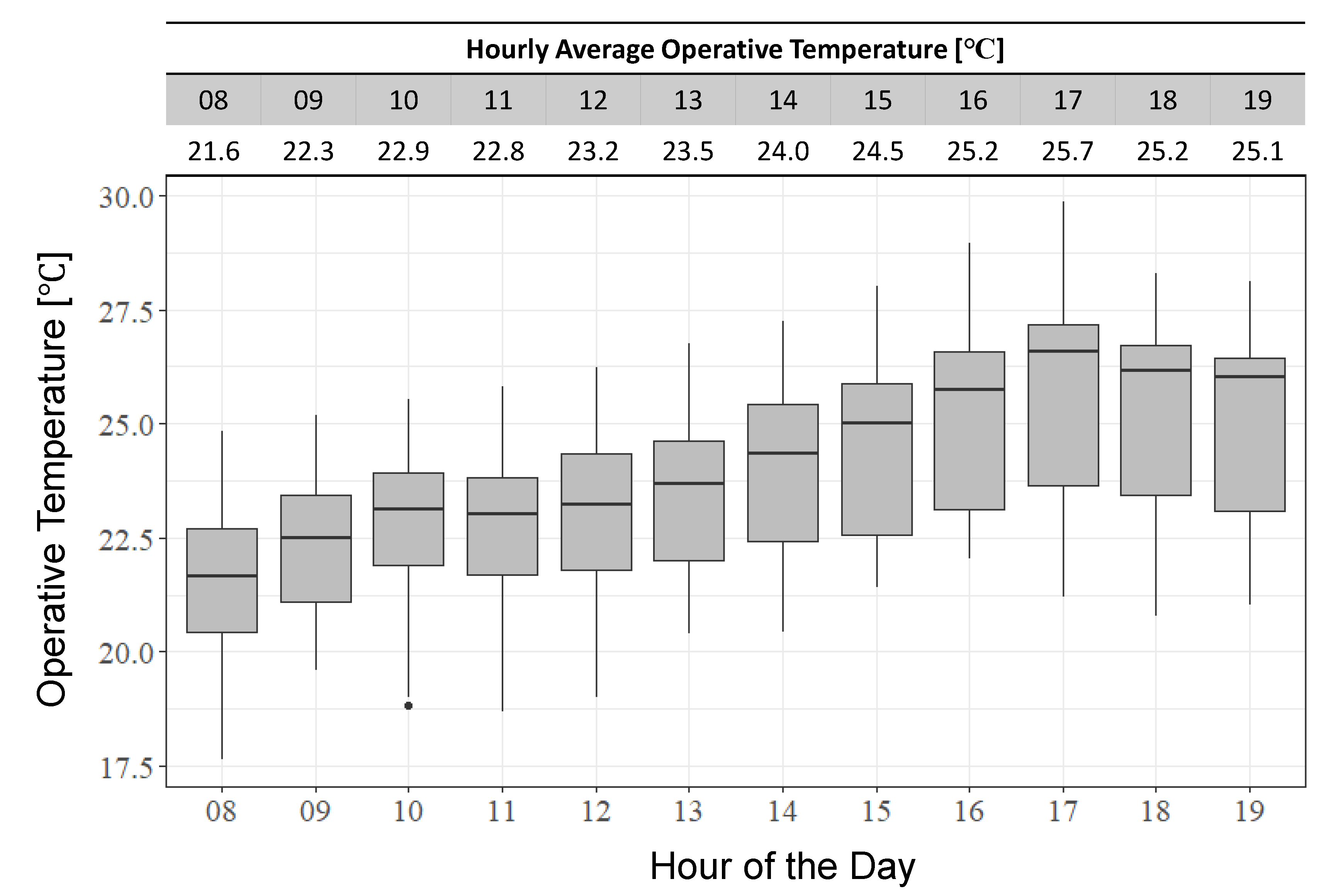
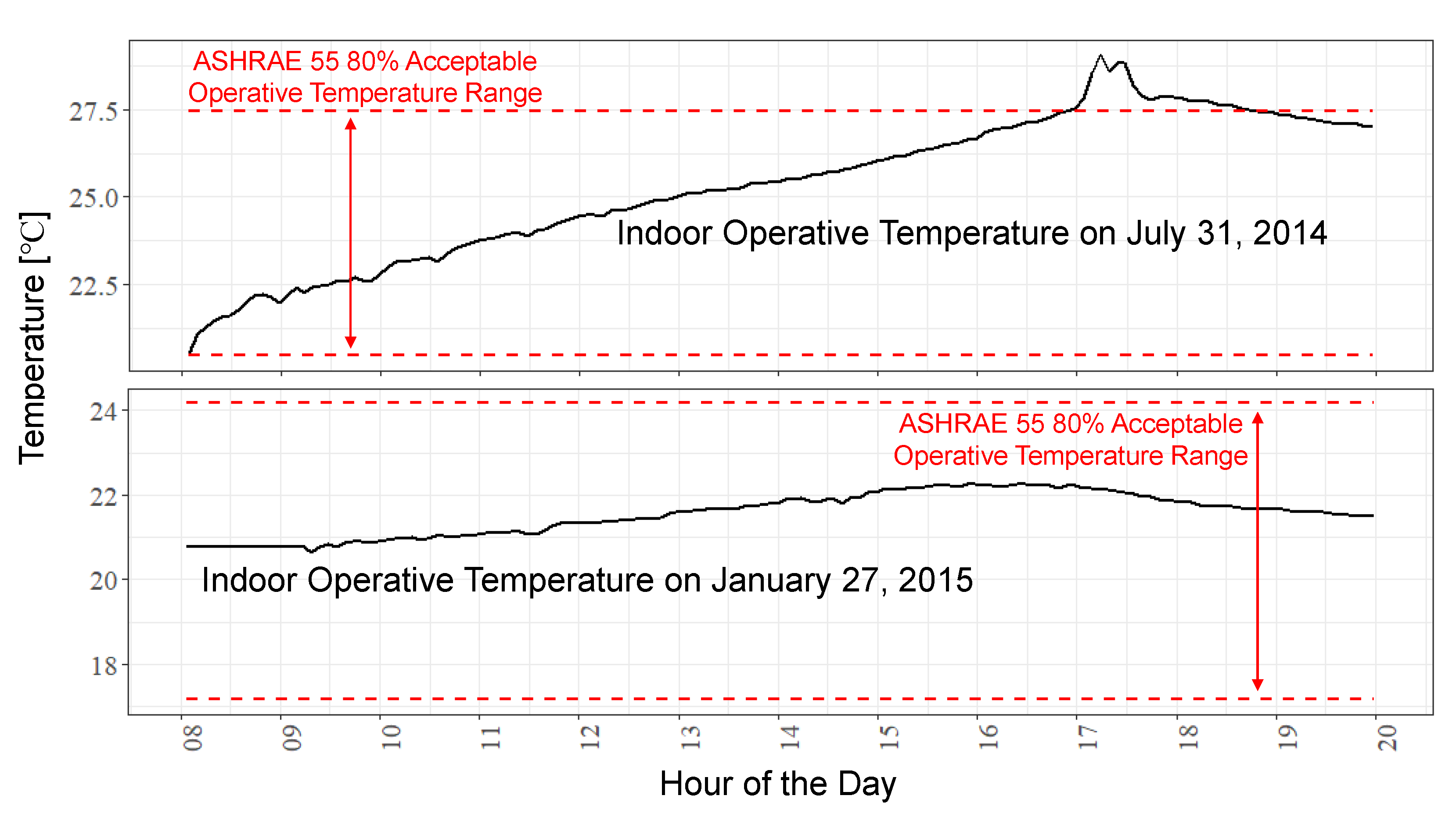
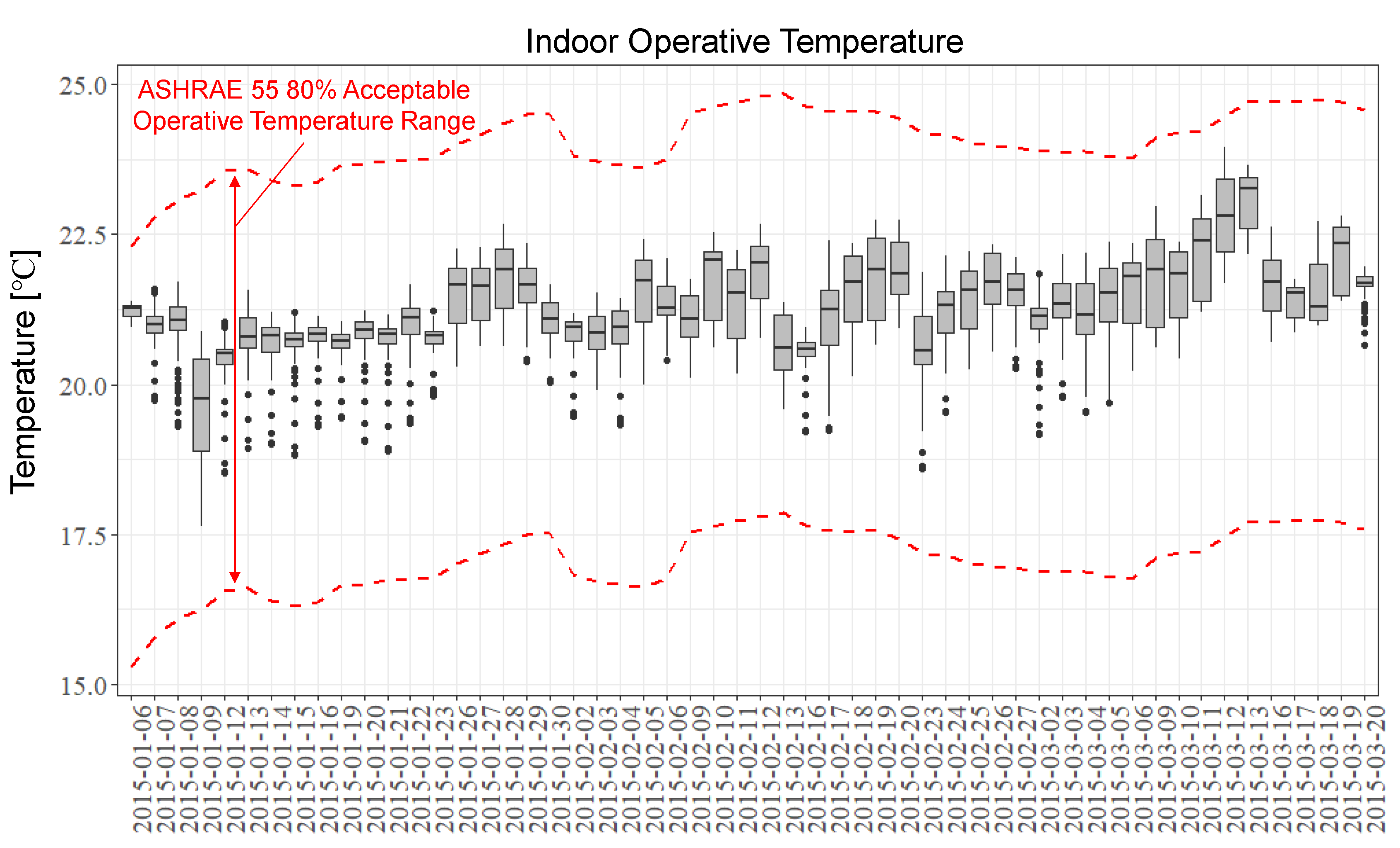
3.1.1. Thermal Comfort Condition

Figure 6, Figure 7 and Figure 8 show box plots of the daily five-minute mean indoor operative temperature during working hours (8 a.m. to 8 p.m.) for summer, fall, and winter, respectively. The indoor operative temperature was not measured directly, although it was the metric used in ASHRAE Standard 55 [32] to determine acceptable thermal conditions in naturally conditioned spaces. Instead, the operative temperature was derived from the air temperature which was measured directly (details were discussed in Section 2.2).
Figure 6 shows that, during the summer months, the indoor operative temperature exceeded the upper and lower 80% acceptability limits occasionally. Further examination showed that the indoor operative temperature dropped below the lower 80% limit mostly during early working hours (e.g., 51% of the measurements that were below the lower 80% limit were observed between 8 a.m. and 9 a.m.). The hourly average operative temperature was in general lower when the day started and kept rising until 5 p.m. (see Figure 9). This can be seen as the effect of night ventilation adopted by the case study building to cool the interior during after work hours from 12 a.m. to 8 a.m. on weekdays. The indoor operative temperature change during working hours was fairly large, which is understandable for a naturally ventilated building. The recorded average temperature change was 4.3 °C, with a maximum difference of 8.6 °C, and a minimum difference of 0.8 °C. Nevertheless, the indoor operative temperature, in general, was maintained within the 80% acceptable range despite the large variations of outdoor air temperature.
As the heating season started, the building was able to maintain the indoor operative temperature within a narrower range as shown in Figure 7 and Figure 8. The occupants’ window opening and closing actions continued through 7 November 2014, after which the windows remained closed. The use of the windows increased the variability of the indoor operative temperature which could be seen from Figure 7. During fall and winter, the operative temperature was always kept within the 80% acceptable range. Figure 10 shows the continued rising of indoor operative temperature in summer, compared to the relatively stable trend in winter.

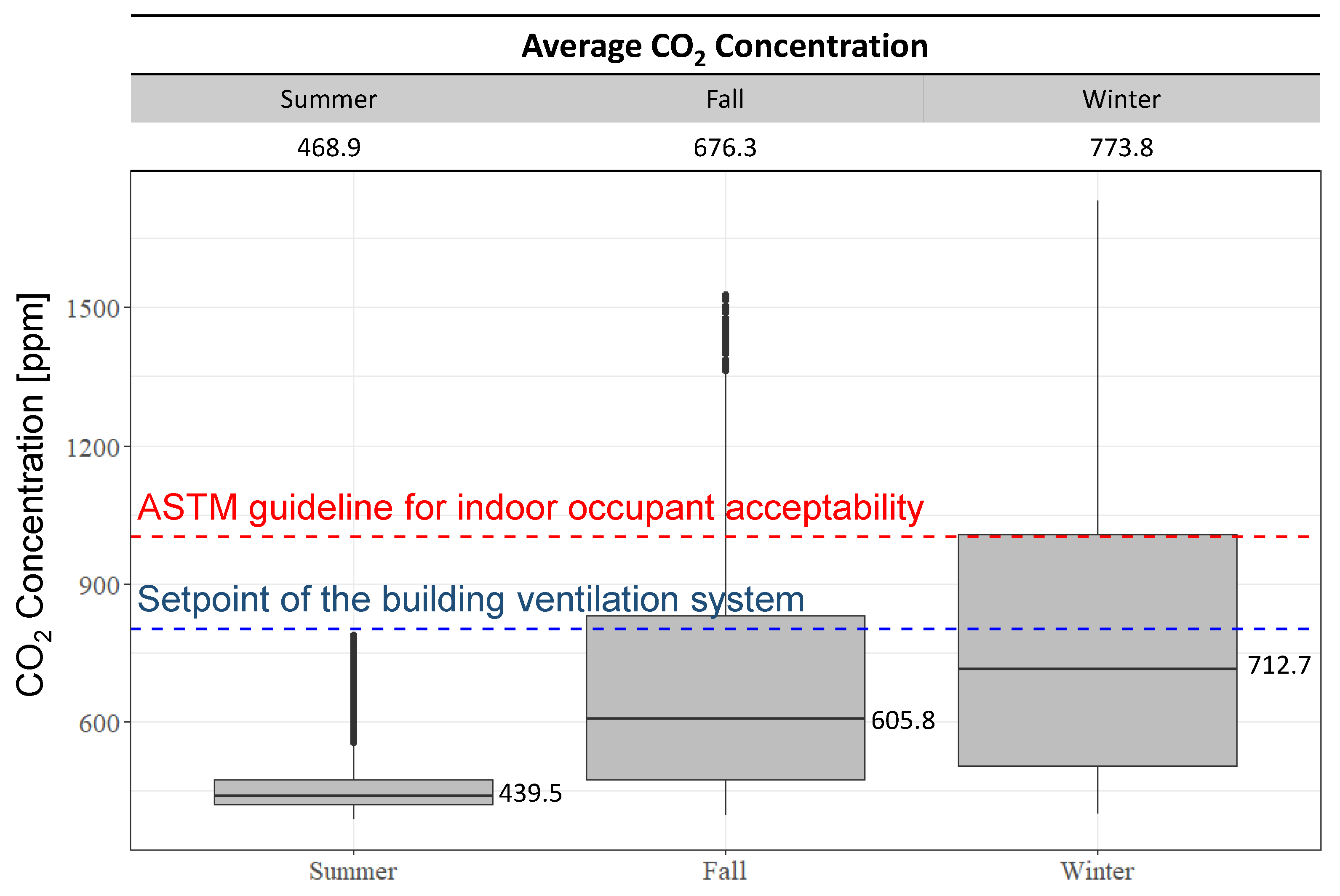
3.1.2. Carbon Dioxide Concentration

Carbon dioxide levels can be harmful to humans at concentrations above 2500 ppm [44]. The American Society for Testing and Materials (ASTM) guideline for indoor occupant acceptability is 1000 ppm, which is calculated as 650 ppm above an assumed 350 ppm outdoor carbon dioxide concentration [45]. The 1000 ppm concentration can be thought of as a metric for odor acceptability [45]. The facilities management of the case study building adopted an 800 ppm set point for the ventilation systems; that is, automated controls for windows and exhaust fans were designed to keep the indoor carbon dioxide concentration below 800 ppm, which assumed a 300 ppm concentration as the outdoor reference [43]. Figure 11 shows the carbon dioxide levels in the instrumented office space during different seasons.
The values of, and variability in, the CO 2 concentrations were much higher in fall and winter, which might be the result of higher occupancy compared to summer. The window opening time also played an important role as the occupants stopped opening windows halfway through the fall season. The 1000 ppm limit recommended by ASTM was well maintained in summer but was exceeded 12% of the time in fall and 26% of the time in winter.

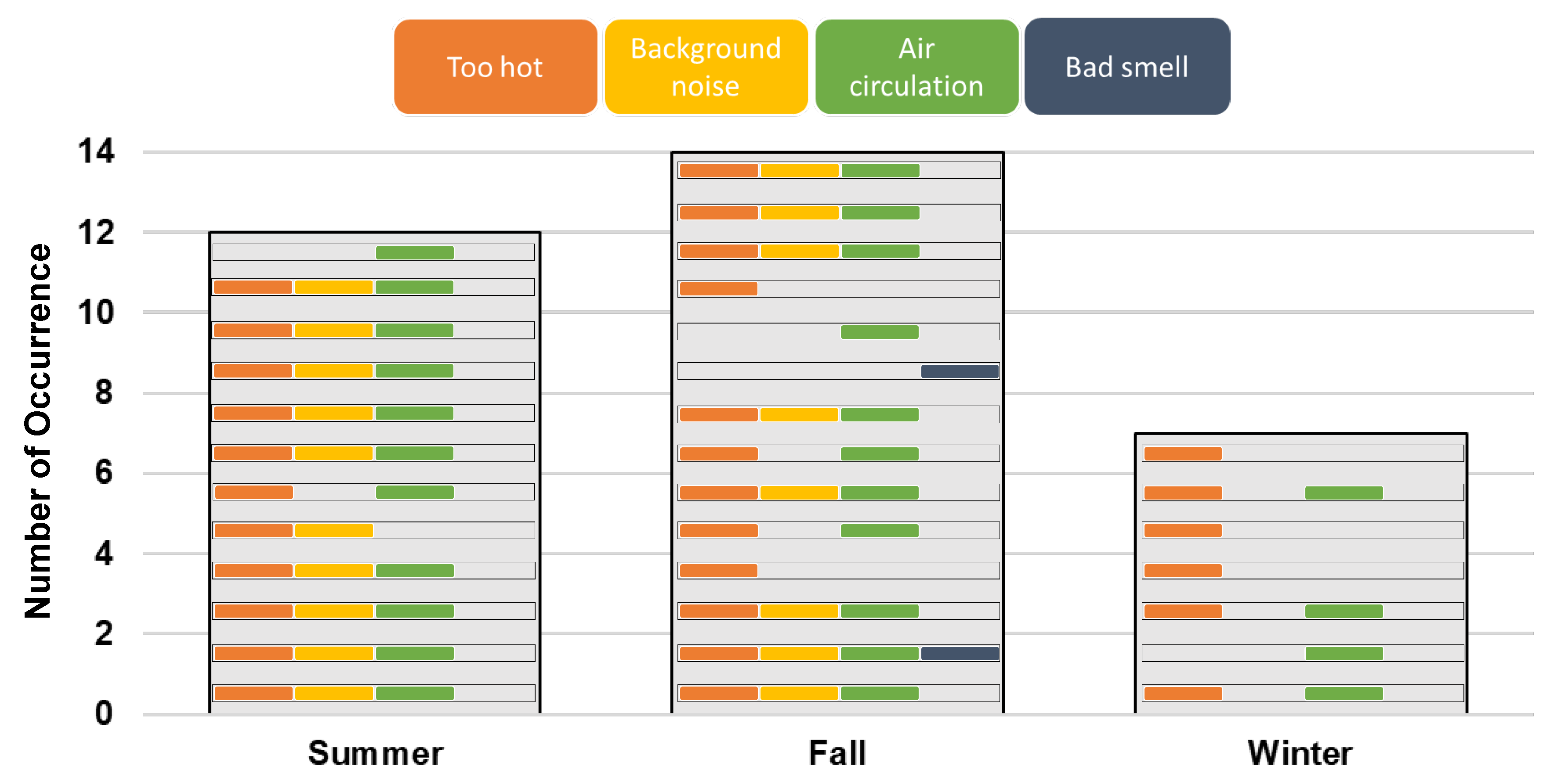
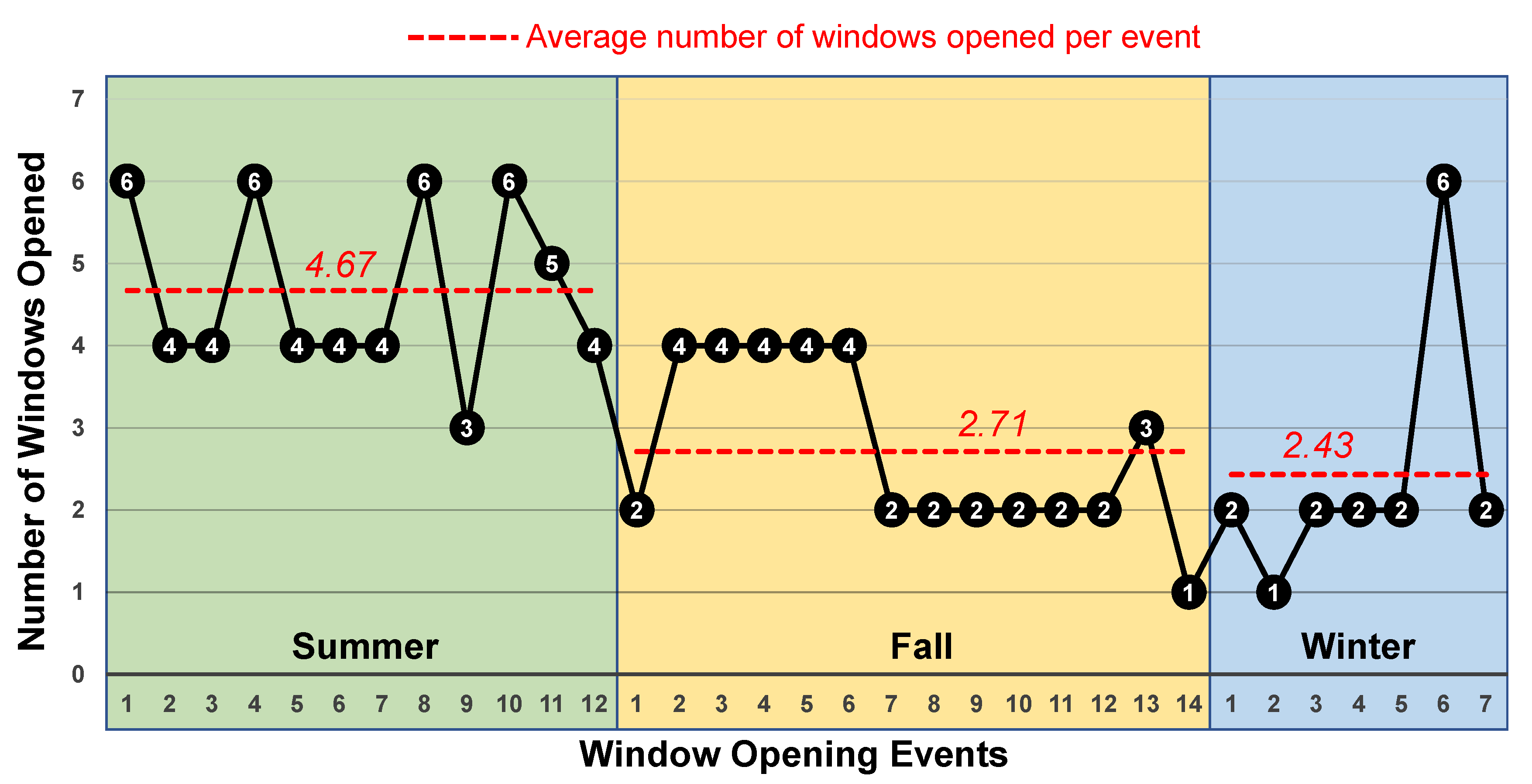
3.2. Window Opening Events

The window opening log form was digitized at the conclusion of the study. The time of each window opening event and the number of windows opened by the occupants were integrated with the indoor and outdoor environmental parameters. On the log form, the occupants were asked to indicate the reason(s) for opening the windows. Four common reasons were listed:
  • the room is too hot;
  • to add background noise;
  • to improve air circulation;
  • to enjoy an outdoor event.
The ‘background noise’ listed above referred to the ambient noise from the outside including but not limited to traffic noise, people talking, bioacoustic noise from animals or birds. This reason was added after some occupants indicated that they would prefer some level of ambient noise while working in the room. The occupants were also allowed to add other reasons for each entry.
Figure 12 shows an overview of the data collected through the log form. The three gray bars correspond to the number of window opening events occurred in summer, fall and winter. It appears that the windows were opened more often in summer and fall than in winter. For each event, the occupants listed one or more reasons for opening the windows, and they are given below:
  • the room is too hot;
  • to add background noise;
  • to improve air circulation;
  • the room has a bad smell.
Except for ‘the room has a bad smell,’ the other reasons were from the options provided on the log form. These four reasons are indicated by different colors in Figure 12. To represent the reasons behind each window opening event, a horizontal strip which consists of at most four colors was created for each event. For example, there were 12 window opening events in the summer (therefore, 12 strips inside the gray bar) and most of the events were driven by three reasons (as indicated by the three-color horizontal strips for 9 out of the 12 strips). In Figure 12, it appears that there were usually two or more reasons behind each window opening event. In summer and fall, the occupants opened the windows to simultaneously cool the room, add background noise, and improve air circulation in 16 out of 26 window opening events (62%), while in winter, when the office space was heated, the need for background noise diminished and windows were opened mostly to cool the room and/or improve air circulation. The number of times each reason was selected by the occupant is shown in Table 4. It can be inferred from these reasons that indoor air or operative temperature, sound level, and indoor air velocity could be the main factors influencing occupants’ WOB.
There were six operable windows in the office. The number of windows opened during each event are plotted in Figure 13. It can be seen that for each opening event, usually more windows were opened in summer (5 windows for each event on average) than fall (3 windows on average) and winter (2 windows on average).

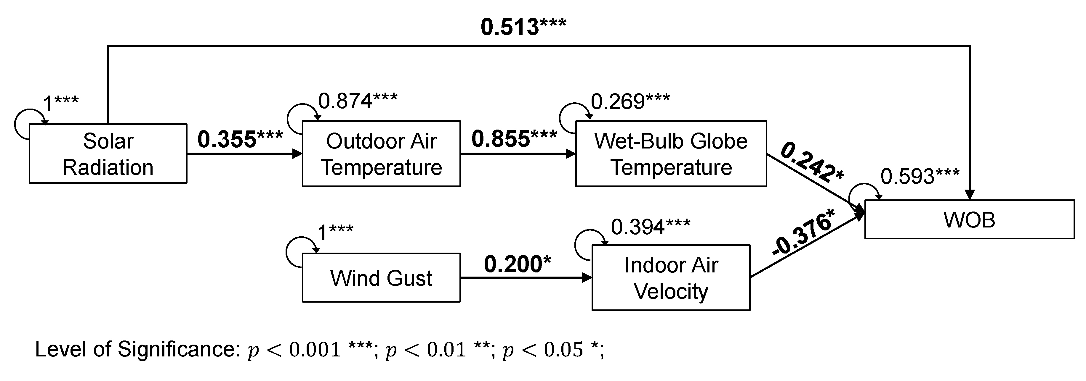
3.3. Structural Equation Model

Figure 14 illustrates the significant structural equation model, showing that multiple factors—solar radiation, outdoor air temperature, indoor wet-bulb globe temperature, outdoor wind gust, and indoor air velocity—affect WOB. In Figure 14, standardized coefficients indicate the relationships between and within parameters. Specifically, the solar radiation positively predicts the WOB ( γ = 0.513 , p < 0.001 ), indicating higher values of solar radiation result in higher probability of WOB. The solar radiation also positively predicts outdoor air temperature ( γ = 0.355 , p < 0.001 ), which subsequently has a positive effect on indoor wet-bulb globe temperature ( γ = 0.855 , p < 0.001 ), which in turn has a positive effect on WOB ( γ = 0.242 , p < 0.05 ). This implies that higher solar radiation results in higher outdoor air temperature and indoor wet-bulb globe temperature, as well as a higher probability of WOB. It corroborates the occupants’ selection of “too hot” as one of the main reasons for opening windows. In addition, the outdoor wind gust has a positive effect on indoor air velocity ( γ = 0.200 , p < 0.05 ) which negatively affects WOB ( γ = - 0.376 , p < 0.05 ). This indicates that higher outdoor wind gust results in higher indoor air velocity, which leads to a lower probability of WOB. It corroborates the occupants’ selection of “air circulation” as one of the main reasons for opening windows, i.e., when the indoor air velocity is low, the occupants tend to open windows to increase air circulation. The SEM model in Figure 14 illustrates only statistically significant relations between variables. The sound level which was one of our main interest showed significant bivariate correlations with outdoor wind speed ( p < 0.05 ) and indoor carbon dioxide concentration ( p < 0.05 ), however, it showed no significant relation with WOB. Given that this study aims to model the relationships between WOB and other variables, we did not include the variables that showed insignificant results with WOB to the main results.
The structural model in Figure 14 also illustrates the mediating effect of indoor environmental parameters (i.e., indoor wet-bulb globe temperature and indoor air velocity) on the relationship between outdoor environmental parameters (i.e., solar radiation, outdoor air temperature, and wind gust) and WOB. Indoor wet-bulb globe temperature mediates the relationships among solar radiation, outdoor air temperature, and WOB. Indoor air velocity also mediates the relationship between wind gust and WOB. Given that the two indoor parameters—indoor wet-bulb globe temperature and indoor air velocity—mediate outdoor environmental parameters and WOB, but the two outdoor parameters—outdoor air temperature and wind gust—cannot predict WOB, the model has full mediation of indoor environmental parameters [36]. The structural model in Figure 14 is supported by the standardized root mean square residual (SRMR) of 0.06, which is lower than the recommended value of 0.08 [46,47].

4. Discussion

The results suggest that naturally ventilated buildings display wide variability in indoor temperatures, particularly in summer months. Although occupant acceptability is subjective, the temperature values exceeded the adaptive model comfort zone stipulated by ASHRAE Standard 55 on more than a few occasions. In general, during summer months, the night ventilation kept the indoor operative temperature close to the lower 80% acceptability limit in the morning. The temperature increased significantly in the afternoon.
The occupants’ WOB is complex, and there is currently no agreement about the reasons people interact with building systems or the driving factors that trigger their decisions [24]. This study was designed to improve the understanding of the interactions among indoor and outdoor environmental parameters and the roles they play in influencing people’s WOB. Many quantitative methods have been used to model WOB such as logistic regression [5,16,18,19,28,29], Markov chains [30], Gauss distribution [30], and deep learning [31]. No studies have been found to apply SEM in the WOB field. SEM is a popular tool among researchers in modeling complex relationships between various explanatory variables and residential energy consumption [48,49,50], as well as in modeling the direct and indirect influence of physical conditions on occupants’ comfort and job satisfaction [51,52,53]. The use of SEM creates opportunities to examine the causal chain of the effect of indoor/outdoor environmental parameters on WOB. Reasons for opening windows recorded by the occupants using the window log form reflected real drivers for WOB from a subjective perspective. The results showed that occupants opened the windows more often during summer and fall as opposed to winter months. Each time the windows were opened, there were usually multiple reasons behind the action, which were mainly “too hot,” “background noise,” and “air circulation.” These reasons corroborate the significant structural equation models except for the “background noise.” As discussed in [24], indoor and outdoor temperatures were still the most cited factors in modeling WOB. Results presented in this study offers a new view which links the indoor and outdoor parameters using the concept of mediation effect rather than treating them separately. It shows that SEM is an effective tool in modeling WOB and the revealed mediation effect of the indoor environmental parameters contributes to the knowledge base of WOB research.
Several limitations are noted for this study. First, the globe temperature was used as an approximation of operative temperature. Given the amount of missing data, the air temperature was eventually used to calculate the globe temperature based on linear regression coefficients. More accurate measurements of operative temperature could improve the results of the adaptive comfort model. Second, although “background noise” was chosen by the occupants as one of the main reasons they opened windows, the SEM results with sound level were not significant. This discrepancy could be attributed to the measurements from the sound meter. It was difficult to differentiate the background noise outside the building from noise generated inside the office solely based on the sound pressure level. A sound meter with frequency analyzer could provide better results and may lead to a significant structural equation model. This study only lasted for eight months with some time gaps. A longer study duration with more recorded window opening events could further improve the structural equation models and may reveal other direct or indirect links between the environmental parameters and WOB.

5. Conclusions

Occupant access to controlling the indoor environment can increase both tenant satisfaction and reduce operational cost. Operable windows are advantageous in that they provide occupants the opportunity to control the indoor environment by increasing the natural ventilation and by decreasing the cooling loads. Motivations for WOB have been extensively studied. Environmental factors, contextual factors, and human factors among others have been identified as influencing factors. Commonly, in all of these previous studies, the physical aspect is repeatedly identified [24].
In this paper, the writers examined the relationship between physical environmental factors and WOB. The results showed that the indoor environmental parameters (such as operative temperature and air velocity) mediated the relationship between outdoor environmental parameters (such as outdoor air temperature and wind gust) and WOB. The indoor wet-bulb globe temperature rose as the solar radiation increased, and subsequently, both parameters affected WOB. Also, higher outdoor wind gust led to higher indoor air velocity, which in turn resulted in a lower chance of occupants opening the window. Modeling the relationship between the indoor/outdoor environmental parameters and WOB revealed the factors influencing the WOB and therefore could be used as predictors of WOB. From a broader implication perspective, the study findings can guide building designers by further justifying and prioritizing the selection of certain building systems. For example, building designers could draw on the results of this study to substantiate the cost and implementation of advanced and innovative window shading devices, such as overhangs and fins that can lower solar heat gains in the summer. This could impact the building’s energy system. Designers can also study the orientation and size of windows in relation to prevailing wind direction and gust. Designers can evaluate the potential to add cross ventilation strategies by assessing the location of windows on both sides of the room or space in terms of wind gust and indoor air velocity. By enhancing our understanding of the relationship between these theoretical parameters, improved design strategies on the mediating parameters can be prioritized and communicated early in the building design phase leading to more informed design decisions.

Author Contributions

The contributions of each author are: conceptualization, A.K. and D.R.; methodology, J.-E.K.; data curation, S.W.; writing—original draft preparation, A.K. and D.R.; writing—review and editing, S.W. and J.-E.K.; visualization, S.W.; funding acquisition, A.K. and D.R.

Funding

This research was funded by the University of Washington’s Green Seed Fund.

Acknowledgments

The authors would like to thank Yiming Liu, engineering technician; Paul Zuchowski, HUB Associate Director; and Carole A. Grayson, JD, Director of Student Legal Services. We would also like to thank all the employees of the Student Legal Services office for filling out the window opening form.

Conflicts of Interest

The authors declare no conflict of interest. The funders had no role in the design of the study; in the collection, analyses, or interpretation of data; in the writing of the manuscript, or in the decision to publish the results.

Abbreviations

The following abbreviations are used in this manuscript:
SEStandard error
StDevStandard deviation
DKolmogorov-Smirnov statistic
CIConfidence interval
Out_RHOutdoor relative humidity (%)
Out_TempOutdoor air temperature (°F)
Out_WindDirOutdoor wind direction (°)
Out_WSpeedOutdoor wind speed (knot)
Out_GustOutdoor wind gust (knot)
Out_RadSolar radiation (watt/m 2 )
Ave_AvIndoor mean air velocity (m/s)
In_CO2Indoor carbon dioxide concentration (ppm)
WBGTIndoor wet-bulb globe temperature (°F)
Sound_dBIndoor sound pressure level (dBA)
WOBFraction of window opened (number of window opened divided by the total of six windows)

References

  1. Brager, G.S.; de Dear, R.J. Thermal adaptation in the built environment: A literature review. Energy Build. 1998, 27, 83–96. [Google Scholar] [CrossRef]
  2. Baker, N.; Standeven, M. Thermal comfort for free-running buildings. Energy Build. 1996, 23, 175–182. [Google Scholar] [CrossRef]
  3. Milne, G.R. The energy implications of a climate-based indoor air temperature standard. In Standards for Thermal Comfort: Indoor Air Temperature Standards for the 21st Century; Nicol, F., Humphreys, M., Sykes, O., Roaf, S., Eds.; Book Section 19; Chapman and Hall: London, UK, 1995; pp. 182–189. [Google Scholar]
  4. Wang, L.; Greenberg, S. Window operation and impacts on building energy consumption. Energy Build. 2015, 92, 313–321. [Google Scholar] [CrossRef]
  5. Rijal, H.B.; Tuohy, P.; Humphreys, M.A.; Nicol, J.F.; Samuel, A.; Clarke, J. Using results from field surveys to predict the effect of open windows on thermal comfort and energy use in buildings. Energy Build. 2007, 39, 823–836. [Google Scholar] [CrossRef]
  6. Fabi, V.; Andersen, R.V.; Corgnati, S.; Olesen, B.W. Occupants’ window opening behaviour: A literature review of factors influencing occupant behaviour and models. Build. Environ. 2012, 58, 188–198. [Google Scholar] [CrossRef]
  7. Choi, J.H.; Loftness, V.; Aziz, A. Post-occupancy evaluation of 20 office buildings as basis for future IEQ standards and guidelines. Energy Build. 2012, 46, 167–175. [Google Scholar] [CrossRef]
  8. van Raaij, W.F.; Verhallen, T.M.M. Patterns of residential energy behavior. J. Econ. Psychol. 1983, 4, 85–106. [Google Scholar] [CrossRef]
  9. Karlsson, F.; Rohdin, P.; Persson, M.L. Measured and predicted energy demand of a low energy building: important aspects when using Building Energy Simulation. Build. Serv. Eng. Res. Technol. 2007, 28, 223–235. [Google Scholar] [CrossRef]
  10. Borgeson, S.; Brager, G. Occupant Control of Windows: Accounting for Human Behavior in Building Simulation; Internal Report; Center for the Built Environment: Berkeley, CA, USA, 2008; Available online: https://escholarship.org/uc/item/5gx2n1zz (accessed on 16 April 2019).
  11. Fritsch, R.; Kohler, A.; Nygard-Ferguson, M.; Scartezzini, J.L. A stochastic model of user behaviour regarding ventilation. Build. Environ. 1990, 25, 173–181. [Google Scholar] [CrossRef]
  12. Haldi, F.; Robinson, D. Interactions with window openings by office occupants. Build. Environ. 2009, 44, 2378–2395. [Google Scholar] [CrossRef]
  13. Herkel, S.; Knapp, U.; Pfafferott, J. Towards a model of user behaviour regarding the manual control of windows in office buildings. Build. Environ. 2008, 43, 588–600. [Google Scholar] [CrossRef]
  14. Nicol, J.F.; Humphreys, M.A. Adaptive thermal comfort and sustainable thermal standards for buildings. Energy Build. 2002, 34, 563–572. [Google Scholar] [CrossRef]
  15. Yun, G.Y.; Steemers, K. Time-dependent occupant behaviour models of window control in summer. Build. Environ. 2008, 43, 1471–1482. [Google Scholar] [CrossRef]
  16. Zhang, Y.; Barrett, P. Factors influencing the occupants’ window opening behaviour in a naturally ventilated office building. Build. Environ. 2012, 50, 125–134. [Google Scholar] [CrossRef]
  17. D’Oca, S.; Hong, T. A data-mining approach to discover patterns of window opening and closing behavior in offices. Build. Environ. 2014, 82, 726–739. [Google Scholar] [CrossRef]
  18. Li, N.; Li, J.; Fan, R.; Jia, H. Probability of occupant operation of windows during transition seasons in office buildings. Renew. Energy 2015, 73, 84–91. [Google Scholar] [CrossRef]
  19. Pan, S.; Xiong, Y.; Han, Y.; Zhang, X.; Xia, L.; Wei, S.; Wu, J.; Han, M. A study on influential factors of occupant window-opening behavior in an office building in China. Build. Environ. 2018, 133, 41–50. [Google Scholar] [CrossRef]
  20. Rijal, H.B.; Samuel, A.; Tuohy, P.; Humphreys, M.A.; Raja, I.A.; Clarke, J.; Nicol, J.F. Development of Adaptive Algorithms for the Operation of Windows, Fans, and Doors to Predict Thermal Comfort and Energy Use in Pakistani Buildings. ASHRAE Trans. 2008, 114, 555–573. [Google Scholar]
  21. Warren, P.R.; Parkins, L.M. Window-opening behaviour in office buildings. Build. Serv. Eng. Res. Technol. 1984, 5, 89–101. [Google Scholar] [CrossRef]
  22. Rijal, H.B.; Humphreys, M.A.; Nicol, J.F. Development of a window opening algorithm based on adaptive thermal comfort to predict occupant behavior in Japanese dwellings. Jpn. Archit. Rev. 2018, 1, 310–321. [Google Scholar] [CrossRef]
  23. Haldi, F.; Robinson, D. On the behaviour and adaptation of office occupants. Build. Environ. 2008, 43, 2163–2177. [Google Scholar] [CrossRef]
  24. Stazi, F.; Naspi, F.; D’Orazio, M. A literature review on driving factors and contextual events influencing occupants’ behaviours in buildings. Build. Environ. 2017, 118, 40–66. [Google Scholar] [CrossRef]
  25. Landsman, J.; Brager, G.; Doctor-Pingel, M. Performance, prediction, optimization, and user behavior of night ventilation. Energy Build. 2018, 166, 60–72. [Google Scholar] [CrossRef]
  26. Andersen, R.; Fabi, V.; Toftum, J.; Corgnati, S.P.; Olesen, B.W. Window opening behaviour modelled from measurements in Danish dwellings. Build. Environ. 2013, 69, 101–113. [Google Scholar] [CrossRef]
  27. Belafi, Z.D.; Naspi, F.; Arnesano, M.; Reith, A.; Revel, G.M. Investigation on window opening and closing behavior in schools through measurements and surveys: A case study in Budapest. Build. Environ. 2018, 143, 523–531. [Google Scholar] [CrossRef]
  28. Yao, M.; Zhao, B. Window opening behavior of occupants in residential buildings in Beijing. Build. Environ. 2017, 124, 441–449. [Google Scholar] [CrossRef]
  29. Shi, Z.; Qian, H.; Zheng, X.; Lv, Z.; Li, Y.; Liu, L.; Nielsen, P.V. Seasonal variation of window opening behaviors in two naturally ventilated hospital wards. Build. Environ. 2018, 130, 85–93. [Google Scholar] [CrossRef]
  30. Pan, S.; Han, Y.; Wei, S.; Wei, Y.; Xia, L.; Xie, L.; Kong, X.; Yu, W. A model based on Gauss Distribution for predicting window behavior in building. Build. Environ. 2019, 149, 210–219. [Google Scholar] [CrossRef]
  31. Markovic, R.; Grintal, E.; Wölki, D.; Frisch, J.; van Treeck, C. Window opening model using deep learning methods. Build. Environ. 2018, 145, 319–329. [Google Scholar] [CrossRef]
  32. ANSI/ASHRAE. Standard 55—Thermal Environmental Conditions for Human Occupancy; ASHRAE: Atlanta, GA, USA, 2013. [Google Scholar]
  33. Chin, W.W. Issues and Opinion on Structural Equation Modeling. MIS Q. 1998, 22, vii–xvi. Available online: https://www.jstor.org/stable/249674 (accessed on 16 April 2019).
  34. Kline, R.B. Principles and Practice of Structural Equation Modeling, 4th ed.; Methodology in the Social Sciences; The Guilford Press: New York, NY, USA, 2016. [Google Scholar]
  35. Vinodh, S.; Joy, D. Structural Equation Modelling of lean manufacturing practices. Int. J. Prod. Res. 2012, 50, 1598–1607. [Google Scholar] [CrossRef]
  36. Rucker, D.D.; Preacher, K.J.; Tormala, Z.L.; Petty, R.E. Mediation Analysis in Social Psychology: Current Practices and New Recommendations. Soc. Personal. Psychol. Compass 2011, 5, 359–371. [Google Scholar] [CrossRef]
  37. Fox, J.; Nie, Z.; Byrnes, J. sem: Structural Equation Models. 2017. Available online: https://CRAN.R-project.org/package=sem (accessed on 16 April 2019).
  38. R Core Team. R: A Language and Environment for Statistical Computing; R Foundation for Statistical Computing: Vienna, Austria, 2018. Available online: https://www.R-project.org/ (accessed on 16 April 2019).
  39. Fox, J. TEACHER’S CORNER: Structural Equation Modeling With the sem Package in R. Struct. Equ. Model. Multidiscip. J. 2006, 13, 465–486. [Google Scholar] [CrossRef]
  40. ASHRAE/USGBC/CIBSE. Performance Measurement Protocols for Commercial Buildings; American Society of Heating, Refrigerating and Air-Conditioning Engineers, Inc.: Atlanta, GA, USA, 2010. [Google Scholar]
  41. Kazkaz, M.; Pavelek, M. Operative Temperature and Globe Temperature. Eng. Mech. 2013, 20, 319–325. [Google Scholar]
  42. Department of Atmospheric Sciences. Rooftop Observations—ATG Building UW; University of Washington: Seattle, WA, USA, 2015; Available online: https://atmos.washington.edu/cgi-bin/list_uw.cgi (accessed on 16 April 2019).
  43. Automated Controls. Asbuilt Drawings Section 230900, University of Washington Husky Union Building; Project Number 08778-20; Automated Controls: Kirkland, WA, USA, 2013. [Google Scholar]
  44. Satish, U.; Mendell, M.J.; Shekhar, K.; Hotchi, T.; Sullivan, D.; Streufert, S.; Fisk, W.J. Is CO2 an Indoor Pollutant? Direct Effects of Low-to-Moderate CO2 Concentrations on Human Decision-Making Performance. Environ. Health Perspect. 2012, 120, 1671–1677. [Google Scholar] [CrossRef] [PubMed]
  45. ASTM International. Standard Guide for Using Indoor Carbon Dioxide Concentrations to Evaluate Indoor Air Quality and Ventilation; ASTM D6245-18; ASTM International: West Conshohocken, PA, USA, 2018. [Google Scholar]
  46. Hooper, D.; Coughlan, J.; Mullen, M. Structural Equation Modelling: Guidelines for Determining Model Fit. J. Bus. Res. Methods 2008, 6, 53–60. [Google Scholar] [CrossRef]
  47. Hu, L.T.; Bentler, P.M. Cutoff criteria for fit indexes in covariance structure analysis: Conventional criteria versus new alternatives. Struct. Equ. Model. Multidiscip. J. 1999, 6, 1–55. [Google Scholar] [CrossRef]
  48. Belaïd, F. Untangling the complexity of the direct and indirect determinants of the residential energy consumption in France: Quantitative analysis using a structural equation modeling approach. Energy Policy 2017, 110, 246–256. [Google Scholar] [CrossRef]
  49. Estiri, H. A structural equation model of energy consumption in the United States: Untangling the complexity of per-capita residential energy use. Energy Res. Soc. Sci. 2015, 6, 109–120. [Google Scholar] [CrossRef]
  50. Kelly, S. Do homes that are more energy efficient consume less energy? A structural equation model of the English residential sector. Energy 2011, 36, 5610–5620. [Google Scholar] [CrossRef]
  51. Aries, M.B.C.; Veitch, J.A.; Newsham, G.R. Windows, view, and office characteristics predict physical and psychological discomfort. J. Environ. Psychol. 2010, 30, 533–541. [Google Scholar] [CrossRef]
  52. Lee, P.J.; Lee, B.K.; Jeon, J.Y.; Zhang, M.; Kang, J. Impact of noise on self-rated job satisfaction and health in open-plan offices: A structural equation modelling approach. Ergonomics 2015, 59, 222–234. [Google Scholar] [CrossRef] [PubMed]
  53. Veitch, J.A.; Charles, K.E.; Farley, K.M.J.; Newsham, G.R. A model of satisfaction with open-plan office conditions: COPE field findings. J. Environ. Psychol. 2007, 27, 177–189. [Google Scholar] [CrossRef]
Figure 1. Framework for a simple mediation model [36].
Buildings 09 00094 g001
Figure 2. The layout of the selected office in the HUB where the indoor environmental parameters and window-opening data were collected.
Buildings 09 00094 g002
Figure 3. Locations of the Atmospheric Sciences Building (ATG) and the Husky Union Building (HUB).
Buildings 09 00094 g003
Figure 4. The layout of the manually operated windows and the form used by the occupants to record window opening and closing actions.
Buildings 09 00094 g004
Figure 5. Conceptual model indicating the mediating effect of indoor variables on the relationship between outdoor variables and WOB.
Buildings 09 00094 g005
Figure 6. Boxplot of 5-min average indoor operative temperature, outdoor air temperature and solar radiation in summer 2014, compared with the 80% acceptability limits defined in ASHRAE Standard 55 [32].
Buildings 09 00094 g006
Figure 7. Boxplot of 5-min average indoor operative temperature in fall 2014, compared with the 80% acceptability limits defined in ASHRAE Standard 55 [32].
Buildings 09 00094 g007
Figure 8. Boxplot of 5-min average indoor operative temperature in winter 2015, compared with the 80% acceptability limits defined in ASHRAE Standard 55 [32].
Buildings 09 00094 g008
Figure 9. Hourly average operative temperatures from 8 a.m. to 8 p.m. recorded during summer months.
Buildings 09 00094 g009
Figure 10. Time series plot of the 5-min average indoor operative temperature of selected two days in summer and winter, compared with the 80% acceptability limits defined in ASHRAE Standard 55 [32].
Buildings 09 00094 g010
Figure 11. Boxplot of recorded 5-min average indoor carbon dioxide concentration levels during three different seasons. The seasonal mean is shown at the top, and the median is printed next to each box.
Buildings 09 00094 g011
Figure 12. The number of window opening events for each season and the reasons for opening windows for each event. Inside the bar of each season, a window opening event is represented by a horizontal strip with different colors corresponding to the reasons behind the window opening, and these strips are ordered by the time each event occurred from bottom to top.
Buildings 09 00094 g012
Figure 13. The number of windows opened (out of 6) for each window opening event.
Buildings 09 00094 g013
Figure 14. Structural equation model of the effect of indoor and outdoor environmental parameters on WOB.
Buildings 09 00094 g014
Table 1. Specifications of equipment used in this study.
ParameterModelAccuracyRange
Air TemperatureREED SD-4214 Thermo-anemometer ± 0.4 °C0∼50 °C
Air VelocityREED SD-4214 Thermo-anemometer ± 2 % + 0.1 m/s0.2∼25 m/s
Globe TemperatureExtech HT30 ± 2.22 °C ( ± 4 F)0∼80 °C
WBGTExtech HT30 ± 2.22 °C ( ± 4 F)0∼50 °C
Relative HumidityFluke 975 Airmeter ± 2 % RH10∼90% RH
CO 2 Fluke 975 Airmeter 2.75 % + 75 ppm0∼5000 ppm
SoundREED SD-4023 Sound Level MeterVaries by Frequency30∼130 dB
Table 2. Linear regression results using indoor globe temperature and air temperature.
SeasonDependent VariablePredictorInterceptCoefficient R 2
SummerGlobe TemperatureAir Temperature0.8570.9320.975
FallGlobe TemperatureAir Temperature−3.2411.0920.966
WinterGlobe TemperatureAir Temperature−3.2491.0960.928
Table 3. Descriptive statistics of measured indoor environmental parameters.
ParameterMeanSE MeanStDevMinMedianMaxD95% CI
Out_RH69.912.0814.2430.0070.0093.000.085(65.73, 74.10)
Out_Temp61.261.167.9541.0061.0083.000.104(58.92, 63.59)
Out_WindDir202.989.4364.6456.00210.00344.000.084(184.00, 221.96)
Out_WSpeed5.040.412.840.005.0011.000.105(4.21, 5.88)
Out_Gust6.230.473.240.006.0013.000.121(5.28, 7.19)
Out_Rad211.030.1206.00.0160.8801.50.118(150.5, 271.5)
Ave_Av0.050.010.100.000.000.420.304(0.02, 0.08)
In_CO2558.528.1193.0416.0504.51319.50.151(501.8, 615.1)
WBGT64.570.453.0957.2064.8069.800.100(63.66, 65.48)
Sound_dB49.110.926.3038.2747.7466.680.088(47.26, 50.96)
WOB0.420.060.390.000.331.000.182(0.31, 0.54)
Table 4. Number of times each reason for opening windows was selected by the occupants during each season.
ReasonSummerFallWinter
The room is too hot11126
To add background noise1080
To improve air circulation11114
The room has a bad smell020

