Abstract
Automated fault detection and diagnosis (AFDD) tools based on machine-learning algorithms hold promise for lowering cost barriers for AFDD in small commercial buildings; however, access to high-quality training data for such algorithms is often difficult to obtain. To fill the gap in this research area, this study covers the development (Part I) and validation (Part II) of fault models that can be used with the building energy modeling software EnergyPlus® and OpenStudio® to generate a cost-effective training data set for developing AFDD algorithms. Part II (this paper) first presents a methodology of validating fault models with OpenStudio and then presents validation results, which are compared against measurements from a reference building. We discuss the results of our experiments with eight different faults in the reference building (a total of 39 different baseline and faulted scenarios), including our methodology for using fault models along with the reference building model to simulate the same faulted scenarios. Then, we present validation of the fault models by comparing results of simulations and experiments either quantitatively or qualitatively.
1. Introduction
In Part I of this study [1], we presented the primary motivation for this research: the development of accurate models for building faults for use in training automated fault detection and diagnosis (AFDD) algorithms. The availability of accurate physical models for building faults advances several key areas of fault detection and diagnosis (FDD) research, including projection of regional or national fault energy impacts [2,3], development of model-based FDD algorithms [4,5], and simulation-based assessment of FDD algorithm performance [6,7]. For large-scale fault impact estimation, availability of reliable fault impact data is a key challenge.
Although data-driven FDD algorithms require large volumes of diverse training data, large data sets of faulty behavior are expensive to obtain experimentally and impractical to acquire from field data. Compared to the field data, simulated training data offer key theoretical advantages in the evaluation of FDD algorithms: the ground truth is known with greater certainty; the cost of generating evaluation samples is low; evaluation samples can be generated for a wide variety of equipment, building types, environmental conditions, and so on; and evaluation data sets may be constructed without significant gaps or biases [7,8]. However, accurate simulation results of faults are difficult to obtain, and rigorous validation is critical if the models are to be trusted [5,7].
Several previous studies focused on capturing the impact of a fault in the building component with experimental measurements. These are either full experimental studies to measure the performance degradation caused by the fault [9,10,11,12,13,14,15,16,17,18,19,20,21,22,23,24,25,26,27,28] or studies focusing on developing fault models or FDD algorithms that use experimental measurements as a basis for development and validation [29,30,31,32,33,34,35,36,37,38,39,40]. These studies cover various faults that occur in buildings at the component level:
- -
- Envelope material [17,24,25,28]
- -
- Air ducts [10]
- -
- Heat exchangers [11,19,23,36]
Or in system-level equipment:
- -
- Chillers [13,31,38]
- -
- Direct expansion units [9,14,18,22,29,30,33,35,39,40]
- -
- Heat pumps [15,16,20]
- -
- Refrigeration systems [21,26]
- -
- Variable air volume systems [12]
- -
- Fan coil units [32]
- -
- Variable refrigerant flow system [34]
- -
- Air-handling units [37].
Although these studies provide useful information related to the individual objectives of each study, only one study focused on fault models that can be directly used in building energy simulations tools such as EnergyPlus® and OpenStudio®. Cheung and Braun [31] developed empirical models of faults (overcharging, excess oil, noncondensable, and condenser fouling) that are common in water-cooled centrifugal chillers. Because chillers are not common in small commercial buildings, however, chiller fault models are not considered in the scope of this study.
In this two-part article series, we present the development and validation of a library of models for faults common in small commercial buildings in the United States. In Part I (Model Development), we described the modeling approach and technical development; in Part II (Model Validation)—this article—we describe an experimental validation methodology for the developed models and the validation results. The remainder of this article is organized as follows: Section 2 presents the validation methodology, Section 3 provides validation results of fault models, and Section 4 and Section 5 include limitations, future work, and conclusions.
2. Methodology
This section includes overall workflow of the entire study as well as detailed descriptions of the building facility used for conducting fault experiments, the workflow of the fault model validation process, and additional tuning processes of the building model based on preliminary building measurement results.
2.1. Overall Workflow
Figure 1 shows the workflow of the study, including prioritization of common faults in small commercial buildings, fault model development (Part I), and fault model validation (Part II). As shown in the figure, fault models [41] developed in Part I were identified as highest priority by Kim, Cai, and Braun [2]; these prioritized fault models have a significant impact in the nationwide energy consumption. Figure 1 also includes fault models that were developed in the earlier phase of this study [42]. Some of these fault models that are applicable in small commercial buildings have been adopted and updated to complete the prioritized fault list. Remaining faults in the list are newly developed; these fault models are refined to have extended capability, such as covering wider modeling objects in the EnergyPlus, compatibility with other fault models within the simulation, and additional feature such as the fault evolution.
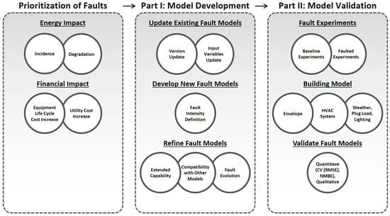
Figure 1.
Overall workflow of this study.
Among faults that were identified as high priority [2], we selected eight different faults (described in Section 2.2) for model validations in this paper, based on the need for model validation and feasibility of experimental implementation. We developed and calibrated a building model—including the envelope; heating, ventilation, and air conditioning (HVAC) system; weather conditions; and internal gains (plug and lighting load)—based on the actual setup of the experimental facility [43,44]. We then used the simulation model to generate results both with and without each fault. While conducting preliminary simulations, we have identified several tuning opportunities in the simulation model that are described in Section 2.4, and these changes were applied in the results in Section 3. In Section 3, we compare the results against the actual experimental measurements. We use the coefficient of variation of the root-mean-square error [CV (RMSE)] and the normalized mean bias error (NMBE) as metrics for the validation as well as qualitative comparisons of component level behaviors. Detailed contents of the validation process are described in Section 2.3.
2.2. Physical Experiments
We conducted our fault research on a two-story flexible research platform (FRP) [43] in Oak Ridge, Tennessee. The building consists of slabs and a steel superstructure, representing a light commercial office building common in the existing U.S. building stock. The FRP is an unoccupied research facility in which occupancy is emulated by process control of lighting, humidifiers for human-based latent loading, and a heater for miscellaneous electrical loads. The emulation minimizes human-occupancy-based interference with the building, which is one of the main sources of uncertainty in building modeling input data. Ground heat transfer is another source of uncertainty because of the unavailability of the deep ground temperature. To reduce this uncertainty, we installed insulation under the ground floor. The added insulation makes the floor-to-ground heat transfer nearly adiabatic. The test building is exposed to natural weather conditions to facilitate research and development of system- and building-level advanced energy efficiency solutions for new and retrofit applications. A dedicated weather station is installed on the roof of the FRP to collect weather data that can be used in performance analysis and energy modeling. Table 1 summarizes the FRP’s general characteristics.

Table 1.
Flexible research platform general characteristics.
The FRP is equipped with a single packaged rooftop unit (RTU) connected to a multizone variable air volume (VAV) system. The RTU has an energy efficiency ratio of 9.6. The connected VAV system serves a total of 10 zones (8 perimeter and 2 core), and each VAV box includes electric resistance reheat. To better monitor and control the outside air introduced to the building, the original intake for the fresh air in the RTU was blocked during experiments (i.e., there was no outside ventilation air). Lighting and occupancy followed schedules and levels found in typical office buildings. During testing, the system operated with the HVAC setpoints noted in Table 1.
The fault experiments consisted of a series of controlled experiments that modified equipment, envelope, and controls in the FRP to impose faults and measure the resulting performance (the data set is publicly available [45]). The experiments were designed to simulate each fault and to validate both the baseline and faulted simulation results. Figure 2 shows the dates of baseline and faulted scenario experiments for all 8 faults. The full set of experiments includes 39 scenarios: 15 baseline scenarios and 24 faulted scenarios. Each fault test imposed a single fault at a fixed fault intensity for a 24-h period, starting at midnight. Faults that occur in the RTU were specifically planned during the cooling season, and the other faults were planned based on the availability of the experimental facility and avoiding the shoulder season where the impact of the fault can be relatively small. If the daily average ambient temperature was above 23.9 °C, the condition of the day was considered as warm weather (cooling season), and if the average temperature was below 12.8 °C, the condition was considered as cool weather (heating season). To verify whether there was a seasonal bias in model prediction, the HVAC setback error fault was tested in both winter and summer seasons. Also, baseline experiments were conducted twice for several faults in order to provide a variety of baseline data for quality control. In general, all experiments used identical internal loads and building controls; however, for some individual faults, specific modifications were made to the general building system configuration.

Figure 2.
Tested dates of baseline and faulted scenarios for eight different faults.
2.3. Validation Workflow
Figure 3 presents the workflow for fault model validation. The workflow was established in the Parametric Analysis Tool (PAT) in OpenStudio [46]. PAT provided an efficient and automated workflow for simulating and validating a total of 39 different faulted and unfaulted scenarios. The workflow requires a calibrated reference building model and fault models for simulating behaviors of the building system under faulted or unfaulted conditions. A calibrated whole-building energy model for the FRP is available from prior modeling efforts [43,44]. The building model developed from these previous studies was used as the initial model for this study. We made additional modifications to the baseline model based on preliminary simulations against the building measurements (see Section 2.4).
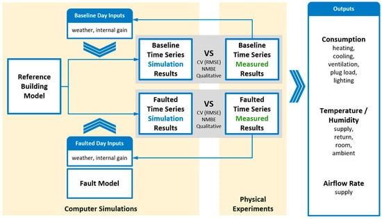
Figure 3.
Fault model validation workflow via the Parametric Analysis Tool.
Because there was only one building physically available for the experiment, experiments were performed sequentially and identical weather conditions did not exist for the baseline and faulted scenarios. Thus, individual baseline experiments were conducted separately for each fault (Figure 2) in order to provide a baseline that represents the same time of year and substantially similar weather conditions as in the fault experiment. Comparisons between the simulation and experimental data are presented separately for baseline and faulted scenarios. To precisely simulate the weather and internal gains in the actual building, the measured weather and internal loads (plug load, occupant, and lighting) were used as inputs for the baseline and faulted simulations. While internal loads were directly defined in the reference building model, the weather measurements from the weather station were converted to EnergPlus weather files (epw file).
Each run of the PAT simulation starts with a minimum 10 days of a warm-up simulation under normal operating conditions (unfaulted; that is, equivalent to the baseline scenario) to minimize the effect of initial conditions defined in the building model. Then, the simulation continues to cover the period that includes all baseline and faulted scenarios. For example, as shown in Figure 2, the condenser fouling experiments were conducted over four different days, including two baseline tests and two faulted tests. Most of the scenarios were tested within seven consecutive days without being interrupted by other fault experiments. The PAT simulation started on August 27, 10 days earlier than the first experiment (25% fouling) and ended on September 2 (second baseline experiment). Except on the dates when a fault was simulated, the building model was simulated based on the normal operating conditions and schedules described in Section 2.2. However, as shown in Figure 2, the experiment schedules for the HVAC setback error fault were split by two other faults (excessive infiltration and nonstandard refrigerant charging) in winter and summer seasons because of scheduling difficulties at the experimental facility. The same validation workflow was used for the HVAC setback error fault assuming that the impact of two other faults was removed after several days of normal operation. Both the simulation and measurement were processed with a 15-min time step.
Figure 3 shows the two model validation activities: validation of the baseline building model and validation of the individual fault models, implemented as OpenStudio or EnergyPlus measures [47]. We used the acceptance criteria established in The American Society of Heating, Refrigerating and Air-Conditioning Engineers (ASHRAE) Guideline 14 [48] for the whole-building electricity consumption for the quantitative validation assessment:
- The CV (RMSE) of the predicted hourly energy consumption shall not exceed 30%.
- The NMBE of the predicted hourly energy consumption shall not exceed ±10%.
CV (RMSE) is a measure of the variance (or spread) in the residual errors, and NMBE is a measure of bias (or average error). Equations of CV (RMSE) and NMBE are shown as Equation (1) and Equation (2), respectively, where n is the total number of data points, y is the actual measurement, is the simulation result, and is the average of y for all time steps.
As shown in Figure 3, there are multiple output parameters available and useful for validating fault models using component-level behavior. These include separate end-use energy consumption for heating, cooling, ventilation, plug load, lighting, and so on, and state measurement outputs (temperature, humidity, and flow rate) in various building HVAC components and thermal zones. Because there are faults that have small impacts on the total building energy consumption level, these detailed end-use consumptions and state parameters are selectively used for the qualitative validation of certain fault models, as described in Section 3.
2.4. Building Model Tuning and Validation Process Modifications
Although Goldwasser et al. [44] made an effort in their study to calibrate the building model against measurements, they found inconsistencies between model results and measurements that could not be explained. In our study, we identified several tuning opportunities in response to issues that were identified. All pertinent details are described in the following subsections; the results shown in Section 3 reflect those changes.
2.4.1. Supply Duct Leakage and VAV Box Configurations
The first opportunity for tuning involved the inherent leakage in the air duct connecting the RTU and terminal VAV boxes. The team conducted a separate measurement to estimate the percentage of the supply air duct leakage in the air system. Table 2 shows airflow measurements taken at the terminal side of all VAV box units (downstream) and at the outlet side of the RTU (upstream). Because there are no permanent airflow sensors installed on the downstream locations, two different tests were conducted with a portable airflow measurement hood—all dampers were set to the minimum position for the minimum airflow operation case and fully open for the maximum airflow operation case. Based on our measurements, the average duct leakage was calculated as 30% of total airflow rate, and this leakage rate level was applied as the downstream leakage fraction in the ZoneHVAC: AirDistributionUnit object in all PAT simulations (baseline and faulted) during the fault model validation.
Table 2.
Airflow measurements for supply air duct leakage prediction.
The actual airflow in the air system is controlled by the supply fan, which operates based on comparing the actual static pressure in the air duct against the static pressure setpoint. In a VAV system, the static pressure varies mostly based on the position of dampers in VAV boxes. Although maximum airflow measurements with all dampers fully open provide useful information regarding the overall capacity of the air system in a full load condition, these are not the exact maximum airflow rates that can be achieved in each VAV box. For example, if only one VAV box damper is fully open and the others are not, the maximum airflow of that VAV box can be higher than when all VAV boxes are fully open. Setting the maximum airflow based on measurements shown in the table will cause a shortage of cooling capacity under certain conditions. Therefore, the modeled maximum airflow for each VAV box was set based on the as-built mechanical drawings for the building. Minimum airflow measurements for each VAV box were directly applied as the minimum airflow settings in the model.
2.4.2. Infiltration in Return Air Plenum
Measurements from the building showed that there is a heat gain (during the summer) or heat loss (during the winter) between thermal zones and the RTU return air temperature. Figure 4 shows a parity plot where each marker represents a comparison between the return air temperature to the RTU and weighted average room air temperature for all 10 rooms at various times. The data points are grouped into summer and winter measurements.

Figure 4.
Temperature difference between room average and RTU return air temperatures.
The summer experiments in the figure represent a data set in which the VAV system was operated with all dampers fully open (condenser fouling tests in 2017); this corresponds to maximum airflow measurements shown in the left side of Table 2. These airflow values were used to calculate the weighted average temperature of 10 thermal zones in the building that was then compared with the direct measurement of the return air temperature at the RTU. The winter experiments shown in the figure are representative of when the VAV system was in heating mode for all thermal zones with all dampers in the minimum position (excessive infiltration tests in 2017). For those cases, the minimum airflow values shown in Table 2 were used to calculate the weighted average temperature. It is clear that the return air temperature to the RTU is higher than the average room temperature in the summer season and lower in the winter season. To capture this effect, the infiltration object in the return air plenum was used as a tuning parameter to match the heat gain or loss between different seasons. By trial and error of comparing the difference between the return air temperature and weighted average temperature with different infiltration levels, the original infiltration level (flow per exterior surface area = 0.001 m/s) in the plenum was reduced by 60% (0.0004 m/s) in the updated building model.
2.4.3. Diffuse Horizontal Irradiance Calculation
The preliminary fault simulation results showed a shortage of cooling capacity in perimeter zones on some occasions. During the capacity shortage periods, perimeter zone temperatures increased to an extreme condition while the RTU operated at its full load condition with maximum airflow. The supply air temperature also rose above its setpoint (12.7 °C) during this period. Because there was no such capacity shortage in the actual building during the corresponding experiment, the model parameters were reviewed to identify the issue.
Figure 5 includes diffuse horizontal irradiance (DHI) plots for eight consecutive days (during which the issue presented itself) from different sources: weather station measurements taken at the FRP, data from the National Solar Radiation Database (NSRDB) [49], and values derived from Equation (3). For the calculated DHI, the global horizontal irradiance (GHI) and direct normal irradiance (DNI) values were taken from FRP weather station data, and the solar zenith angle () was adopted from the NSRDB for the same location.
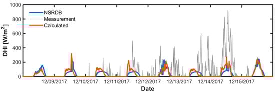
Figure 5.
Difference between measured and calculated diffuse horizontal irradiance (DHI).
As shown in Figure 5, the measured DHI rises above 800 W/m2 at peak and to around 600 W/m2 during nights between December 12 and 15. Because direct normal irradiance can reach up to 1000 W/m2 when the sun is at its zenith, the DHI measurements from the building location are not plausible. Because the issue only occurred during a short period in the winter season measurement, it is unclear exactly what caused it. Although this affected only a small portion of the validation data set, the measured DHI values were replaced with the calculated values in all cases to ensure modeling consistency.
2.4.4. Other Preprocess Modifications
In addition to the previously described modifications to the reference building model and weather file that were applied to all validation scenarios, additional modifications were selectively applied to certain type of faults.
Room temperature setpoint mapped to the measurements: In an actual VAV system, room temperature is controlled at the VAV box by modulating the cooling or heating capacity with the damper or heating coil, respectively. Each VAV box has a controller for sensing the room temperature and modulates conditioning capacity by comparing the room temperature against the room temperature setpoint. If the quality of the VAV box and tuning of its controller are not sufficiently sophisticated, precise room temperature control cannot be realized even when there is sufficient heating or cooling capacity. On the simulation side, room temperatures are controlled perfectly when there is sufficient conditioning capacity (damper position or heating coil run time fraction is set to automatically meet the cooling or heating setpoint for a particular timestep). Fixed room temperature setpoints for heating and cooling are imposed in the actual building during experiments. However, the experimental data showed deviations between measured room temperatures and the corresponding setpoints. Such deviations can be a critical aspect of the building dynamics if the fault affects the room temperature directly (e.g., thermostat bias). However, for faults that do not affect zone temperature, matching the measured noise of the VAV box’s control precision on the simulation side helps isolate fault impact. For this reason, validations of faults such as HVAC setback error, lighting setback error, and RTU faults (condenser fouling and nonstandard refrigerant charging) were performed by using room temperature setpoints based on actual room temperature measurements. Fault model validation scenarios affected by this modification are indicated in Table 3 in Section 3.
Table 3.
Validation results and preprocessing modifications for each fault model validation scenario.
Supply air temperature setpoint mapped to the measurements: A fixed supply air temperature setpoint was imposed in the building experiments. However, precision of supply air temperature control is dependent on the RTU’s control capability. Similar to room temperature control, supply air temperature is also controlled perfectly in EnergyPlus when conditioning capacity is sufficient. Similar to the room temperature setpoint case, mapping simulation supply air temperature setpoint to measured values enables better isolation of certain faults. However, there are faults that can significantly increase the cooling load on the cooling coil, which can result in increased supply air temperature. These include excessive infiltration, return air duct leakage, and stuck economizer damper faults. Apart from these three faults, the supply air temperature experimental measurements were imposed as supply air temperature setpoints in PAT simulations. Fault models affected by this modification are indicated in Table 3.
Converting the lighting power measurements to a schedule object in EnergyPlus: In a regular simulation case where the lighting schedule is predefined in OpenStudio, the lighting setback fault model directly modifies the lighting schedule defined in the building model. However, the PAT simulation setup shown in Figure 3 was constructed by reading the lighting profile from the measurement file and rerouting it into the building model. The sequence of reading and modifying the schedule is not properly ordered in the PAT simulation; thus, the lighting setback error fault model was not originally able to read in the lighting profile extracted from FRP measurement. For this reason, the measured lighting power profile was converted manually to a schedule object in the building model prior to lighting setback fault validation.
3. Fault Model Validation Results
The overall validation results and model preprocessing modifications for all fault model validation scenarios are summarized in Table 3. The validation results in this table are presented with CV (RMSE) and NMBE by comparing the results of total building electricity consumptions between actual measurements and model predictions for each scenario. The graphical bars indicate the results of CV (RMSE) and NMBE for each scenario measured against the target error levels (CV [RMSE] = 30%/NMBE = ±10%). A one-hour time step resolution is used for the CV (RMSE) and NMBE calculations, consistent with ASHRAE Guideline 14. CV (RMSE) and NMBE for most of the scenarios are within the target; others are close but not within the target.
These results show that the scale of the model prediction with the building envelope model, HVAC model, and fault models is within a reasonable boundary. However, the results in this table do not guarantee the validity of all fault models. There are specific details that need to be addressed for certain fault models to fully verify model validity. Additionally, variation in CV (RMSE) and NMBE values for baseline results across different faults indicate the presence of noise and uncertainty within the system stemming from the inherent differences between actual and modeled operation. This, combined with the fact that many of the faults have minimal impact on whole-building electricity use, makes it impractical to evaluate models solely using the chosen error metrics of the whole-building electricity consumption. Therefore, we also performed qualitative validation of each fault model. These results are addressed in the following subsections along with experimental configurations for each fault. Table A1 in Appendix A summarizes detailed configurations of each fault experiment, including fault intensity definition, fault imposition method, tested date, average daily ambient temperature, and exceptional condition. The baseline results illustrated in tables and figures in the following subsections represent Baseline 1 measurements listed in Figure 2 and Table 3. Detailed description of each fault model can be found in Part I of this article series [1].
An additional modification was made in the following subsections to the original CV (RMSE) and NMBE to better characterize the agreement between experiments and simulations and to understand the impact of each parameter on the building-level energy consumption. For example, in the heating season, the cooling demand is almost negligible compared to the heating demand. Because the uncertainty of predicting the building energy consumption remains constant in the simulation, the CV (RMSE) and NMBE increase significantly for the cooling consumption in the heating season. Although this can be interpreted as quantitatively poor agreement of cooling energy consumption between the measurement and simulation, this does not mean the behavior of the building system is poorly predicted because the absolute scale and the impact of that small energy consumption are negligible. In order to compare the agreement level of three major energy consumption categories (total building consumption, total cooling consumption, and total heating consumption) based on the same reference scale, modified CV (RMSE) (CV* [RMSE]) and NMBE (NMBE*) are used that replace the variable in Equations (1) and (2) of cooling and heating consumptions with of the total building electricity consumption, meaning that the modified metrics are normalized with respect to the total building energy consumption rather than the energy consumption of the heating and cooling systems.
3.1. HVAC Setback Error
While the normal setback hours for the entire operating period are between 10 p.m. and 7 a.m., the controller was directly modified to emulate three different setback error scenarios: delayed onset, early termination, and no setback. Each fault scenario for these fault experiments was tested twice, once in the heating season and once in the cooling season. To capture contiguous overnight setback periods for each of the fault tests and to avoid transient effects at each end of the test period, the operator imposed the fault prior to the start of the overnight setback period on the day preceding the fault test and removed the fault after the end of the overnight setback period on the day following the fault test. This was an exception to the general test procedure (besides the lighting setback error fault), in which fault testing began and ended at midnight.
Table 4 shows CV (RMSE) and NMBE values for a number of model outputs within the building system for combined summer and winter periods. In Table 4, cells are highlighted when the CV (RMSE) and NMBE (as well as CV* [RMSE] and NMBE*) predictions are outside the targets (CV [RMSE] = 30% and NMBE = ±10%). Most of the outputs are predicted well against measurements, but the humidity ratio of the return and supply air and latent cooling capacity are not. The poor prediction of the humidity level in thermal zones is also discussed in the initial calibration of the building model [44]. This is one of the model limitations that has not been solved in this study and needs to be improved by improving the moisture balance model in the EnergyPlus and sensible heat ratio prediction in the cooling coil model. Although the validation of the HVAC setback model does not require precise agreement for the building’s humidity prediction, there are other faults (such as faults in the RTU) where the humidity level is important for properly predicting the latent cooling capacity. Because the setpoint of the room and supply air temperature were simulated based on actual measurements, the predictions for these two outputs are within 8% of CV (RMSE). The results show infinite values of CV (RMSE) and NMBE for the latent cooling capacity predictions, and this is because of the zero dehumidification measurements in the winter season. Because the absolute scale of the latent load is relatively small (in both winter and summer) compared to the sensible load, the total cooling capacity predictions are within the target compared to measurements.
Table 4.
CV (RMSE) and NMBE Calculations for Detailed Model Outputs: HVAC Setback Error (Average of Winter and Summer).
Figure 6 shows total electricity consumption (sensor accuracy = ±0.5% of reading) of the building for each winter season scenario. It is clear from these results that delayed onset, early termination, and no overnight setback faults are properly implemented in the model. Because the normal setback starts at 10 p.m., 3 h of delay in setback causes the HVAC system to operate until the end of the day (Figure 6b). Terminating the setback 3 h earlier than the normal operation causes the HVAC system to operate at 4 a.m. (Figure 6c). The HVAC system operates the entire day when the setback is not applied (Figure 6d). The profiles of the total energy consumption predictions agree well with the measurement.

Figure 6.
Total building electricity consumptions of baseline and faulted scenarios: HVAC setback error (winter). (a) baseline; (b) delayed onset; (c) early termination; (d) no setback.
Figure 7 shows the same time series plots, but for the summer season experiments and simulations. The magnitudes of energy consumption are slightly reduced compared to winter results. Based on model predictions shown in Figure 6 and Figure 7, the building model reasonably captures the seasonal difference between heating and cooling seasons.

Figure 7.
Total building electricity consumptions of baseline and faulted scenarios: HVAC setback error (summer). (a) baseline; (b) delayed onset; (c) early termination; (d) no setback.
3.2. Lighting Setback Error
Fault definitions and the method of imposing the fault on the building are similar to the previous HVAC setback error fault. Lighting setback error faults were also imposed ahead of the actual fault testing date and removed the day after the testing date to avoid transient effects at transitions. Table 5 presents CV (RMSE) and NMBE results of detailed model outputs for all scenarios. The prediction trend is similar to the HVAC setback error results. The poor predictions of the humidity ratio and latent load cooling capacity as discussed in Section 3.1 are also shown in this table. A lighting column is included, and corresponding CV (RMSE) and NMBE values were calculated. The heating energy consumption is overpredicted (negative NMBE) compared to the measurement for the no setback scenario, which resulted in slightly higher CV (RMSE) above the target limit.
Table 5.
CV (RMSE) and NMBE Calculations for Detailed Model Outputs: Lighting Setback Error.
Figure 8 shows lighting power comparisons between experiments (sensor accuracy = ±0.5% of reading) and simulations for each scenario. The baseline measurements and model results in Figure 8a match perfectly because the actual measurement was fed into the model. In addition, the faulted lighting power profiles imposed by the fault model in Figure 8b–d agree well with the actual faulted measurements. Small deviations between the measurements and model predictions are a result of limitations in the model (i.e., the model simplifies the profile when there are multiple changes in the value within an extended time frame) and sensitivity of the lighting power control and sensor measurement.

Figure 8.
Lighting power consumptions of baseline and faulted scenarios: lighting setback error. (a) baseline; (b) delayed onset; (c) early termination; (d) no setback.
Figure 9 shows total electricity consumption time series for all scenarios and comparisons between experiments (sensor accuracy = ±0.5% of reading) and model predictions. All model predictions show good agreement against the experimental measurements. However, impacts of lighting setback fault scenarios are not readily apparent in these graphs when comparing model results with and without the fault. This is one example of a fault in which the fault impact is very small compared to the whole-building energy consumption. In Figure 8, the lighting power consumption is on the order of 1–3 kW, while the total consumption in the building level reaches 20 kW in the summer and 30 kW in the winter.
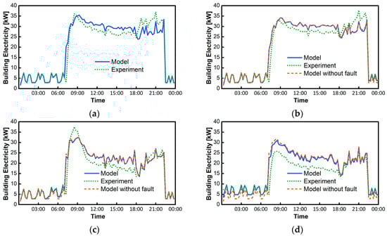
Figure 9.
Total building electricity consumptions of baseline and faulted scenarios: lighting setback error. (a) baseline; (b) delayed onset; (c) early termination; (d) no setback.
3.3. Condenser Fouling
For the condenser fouling and return air duct leakage faults, the fault intensity is defined at the full load condition (supply fan at 100% speed and all VAV dampers fully open) and referenced to the design airflow rate. Thus, fault intensities for these faults are measured based on the full load condition prior to the actual experiments, and actual experiments are also conducted under the full load condition. The operator covered the condenser coil with a blocking media (i.e., meshes with different perforation levels) to reduce the airflow, remeasured the surface air velocity, and adjusted the blocking media until the target airflow reductions were achieved. The media thereafter remained unchanged for the duration of each test. Because the HVAC system was forced to operate under the full load condition, additional VAV heating was provided to thermal zones to prevent overcooling.
Table 6 shows the CV (RMSE) and NMBE values for detailed building system parameters for the condenser fouling fault scenarios. Energy consumption predictions for the total building, heating, and cooling agree well with actual measurements based on CV (RMSE), but there are some biased results in terms of NMBE in the 28% and 58% fouled scenarios. Besides the poor humidity prediction in the EnergyPlus building model, another limitation that is not solved in this study is the accuracy of the latent cooling capacity prediction of the two-stage direct expansion (DX) unit model. The DX unit model in EnergyPlus requires nominal values (rated capacity, rated coefficient of performance [COP], rated sensible heat ratio, and rated flow rate) along with performance maps that adjust the nominal performances of the DX unit depending on different operating conditions (ambient temperature, wet-bulb temperature to evaporator inlet, and part load ratio). A separate study was conducted to develop these performance maps for the two-stage DX unit [50]. Total cooling capacity and power consumption estimations of the DX unit agree well with measurements, whereas the sensible heat ratio prediction affecting the latent cooling capacity still needs some improvement. The impact of the condenser fouling fault is negligible in terms of the building-level energy consumption. As a result, validation focused on RTU performance measures.
Table 6.
CV (RMSE) and NMBE Calculations for Detailed Model Outputs: Condenser Fouling.
The fault model was evaluated in terms the relative RTU performance differences between the baseline and faulted scenarios. Figure 10 shows measurements (COP uncertainty ≈ 3% of reading) and model predictions of COP reductions in faulted scenarios compared to the baseline measurement and model prediction, respectively. This way of isolating the degraded performance of the DX unit eliminates the DX unit’s performance difference between the actual unit and model. The degradation trend is correct, but the magnitude of the modeled degradation is incorrect. In Figure 10, in the 28% fouling scenario, the model slightly underpredicts the COP reduction compared to the measurement. In the 58% fouling scenario, the model significantly underpredicts the COP reduction. The condenser fouling and nonstandard refrigerant charging fault models include regression models that are trained with training data from multiple sources [42], but not with data from the specific RTU used in the validation experiments. Thus, the deviation stems from the degradation difference between training data and actual DX unit equipment tested in the building. Thus, improvements can be made for this fault model by utilizing a larger and more representative training data set or developing an extended regression model that can capture additional operating parameters that may have caused differences in results. The peak values at the beginning and end of the measurements are a result of the transient response during the transition between unoccupied hours and occupied hours.

Figure 10.
Reduction of COP in faulted scenarios: condenser fouling. (a) 28% fouling; (b) 58% fouling.
3.4. Nonstandard Refrigerant Charging
Prior to executing the fault tests, the operator evacuated the RTU’s refrigerant circuit and recharged it to the nominal (manufacturer-specified) value. This nominal value was used as the baseline for subsequent fault tests. To impose a nonstandard refrigerant charge level, the operator evacuated and recharged the RTU’s refrigerant circuit with a mass of refrigerant that differed from the nominal value by the specified fault intensity. No exceptional experimental conditions were applied during these fault experiments, and all operating conditions and schedules followed the normal condition (besides refrigerant charge levels and weather conditions) described in Section 2.2.
Table 7 shows the CV (RMSE) and NMBE results of detailed model outputs for the nonstandard refrigerant charging fault. Prediction accuracies are similar to the results of the condenser fouling, but with slightly more biased predictions (e.g., heating energy consumption and airflow rate).
Table 7.
CV (RMSE) and NMBE calculations for detailed model outputs: Nonstandard refrigerant charging.
Because the impact of a nonstandard refrigerant charging fault is relatively small compared to the whole-building energy consumption, COP reductions of different fault scenarios are used for the validation, as shown in Figure 11. Besides the transient response difference between measurements (COP uncertainty ≈ 3% of reading) and simulations early in the occupied period, the scale and overall profile of COP reduction predictions for all scenarios show good agreement with the measurements.

Figure 11.
Reduction of COP in faulted scenarios: nonstandard refrigerant charging. (a) 15% undercharge; (b) 30% undercharge; (c) 15% overcharge.
3.5. Thermostat Measurement Bias
A thermostat bias of +2.2 °C is defined as a thermostat reading 2.2 °C higher than the actual zone temperature. Based on the definition, the experiments were conducted by changing the room setpoint temperature instead of imposing a bias in the thermostat reading. For example, the thermostat bias of +2.2 °C was simulated by decreasing the zone setpoint temperature by 2.2 °C. The operator used thermostats in rooms 105, 106, 205, and 206 to emulate the thermostat measurement bias of each scenario. These rooms were selected to produce the greatest (most readily measurable) fault impact; all these rooms face south and have a larger floor area compared to the other rooms.
Table 8 shows the CV (RMSE) and NMBE results of detailed model outputs for all scenarios of the thermostat measurement bias fault. The total building, heating, and cooling energy consumption predictions are within the target based on CV* (RMSE), with slight underpredictions shown in NMBE*. As summarized in Table 3, the setpoints for room temperatures in the simulations for this fault were fixed values defined in Table 1 rather than actual room temperatures from the experiments. Although predictions of total building, heating, and cooling energy did not change significantly, the CV (RMSE) and NMBE results of room temperatures were slightly higher than the results when measured values were imposed as the room temperature setpoint. The impact of tested fault scenarios was not significant in terms of the building level energy consumption and validation of the model focused on room temperature controls.
Table 8.
CV (RMSE) and NMBE calculations for detailed model outputs: Thermostat measurement bias.
Figure 12 shows room temperature comparisons (for rooms 105, 106, 205, and 206) between experiments (sensor accuracy = ±0.1 °C at 23 °C) and simulations where thermostats were biased with −2.2 °C (equivalent to the thermostat setpoint increased by 2.2 °C) for two scenarios: thermostat bias in two rooms (105 and 205) and four rooms (105, 106, 205, and 206). In this figure, results in Figure 12c,g are the only rooms where the thermostat bias was not applied. Because it is difficult to calibrate an individual room’s thermal behavior accurately with the model, temperature differences between model predictions and measurements vary among the different rooms. Rooms on the second floor (205 and 206) have better agreement compared to rooms on the first floor (rooms 105 and 106). As shown with these results, fault models that only modify existing variables in EnergyPlus rely on the accuracy of the building model in terms of predicting its impact.

Figure 12.
Room temperature comparisons between experiments and simulations: thermostat measurement bias. (a) −2.2 °C bias in two rooms: room 105; (b) −2.2 °C bias in four rooms: room 105; (c) −2.2 °C bias in two rooms: room 106; (d) −2.2 °C bias in four rooms: room 106; (e) −2.2 °C bias in two rooms: room 205; (f) −2.2 °C bias in four rooms: room 205; (g) −2.2 °C bias in two rooms: room 206; (h) −2.2 °C bias in four rooms: room 206.
Based on results of rooms on the second floor (Figure 12e–h), the −2.2 °C bias was well predicted compared to measurements. The model captures both early and late reheating demand and provides less cooling during midday. However, while the prediction of the temperature in room 206 (Figure 12g) shows almost perfect control along the setpoint, the temperature prediction in room 106 (Figure 12c) is not close to the setpoint because of the insufficient cooling capacity limited by the maximum airflow defined in Table 2. Based on results shown in this section, the fault model accurately captures demands of reheating and cooling throughout the day, but requires a more accurate building model in order to predict individual room temperatures precisely.
3.6. Excessive Infiltration Through the Building Envelope
Prior to the actual fault tests, we conducted a series of blower door tests to measure the infiltration levels for baseline and faulted scenarios. The HVAC system was turned off during these tests. Table 9 includes results of the blower door tests for different scenarios. For each fault scenario, the operator repeatedly conducted a blower door test while adjusting window openings in two rooms (rooms 106 and 204) to increase the effective leakage area by an amount that achieved the specified fault intensity. The vertical lengths of window openings of each room in Table 9 derived from these tests then remained unchanged for the duration of each fault experiment. In order to increase the impact of the infiltration on the building, relatively colder days (daily average outdoor air temperature less than 7.2 °C) were selected for all experiments.
Table 9.
Blower door test results for each scenario.
The infiltration fault model uses standard infiltration objects that are already implemented in EnergyPlus. EnergyPlus infiltration models can use a fixed infiltration rate for the entire simulation period or can include some level of variation against the design infiltration rate by using a correlation model that includes effects of the indoor and outdoor temperature difference and wind speed. However, there are many more factors that influence infiltration or exfiltration in actual buildings. The infiltration or exfiltration will occur based on the pressure difference between the indoor and outdoor environment; this pressure can also vary depending on the opening/closing of windows/doors, cracks or leaks through the building envelope, intensity of the building stack effect, and so on. All these physical properties that drive the building’s infiltration/exfiltration level are difficult to completely implement within the approach that is currently used in the EnergyPlus simulation. However, to make the infiltration model as detailed as possible, we used the infiltration correlation model in the simulation [44]. Table 10 and Figure 13 show validation results of detailed model outputs and total building energy consumption profiles for all scenarios. As shown in Table 10, the total building energy consumption predictions are above the target for both baseline and +20% infiltration scenarios. The CV (RMSE) of heating energy prediction is high in the baseline scenario, and room temperature predictions are relatively poor compared to previous validation results. In this fault model validation, fixed setpoints were used instead of actual measurements for both room temperature and supply air temperature setpoints, as described in Section 2.4.4.
Table 10.
CV (RMSE) and NMBE Calculations for Detailed Model Outputs: Excessive Infiltration Through the Building Envelope.

Figure 13.
Total building electricity consumptions of baseline and faulted scenarios: Excessive infiltration through the building envelope. (a) baseline; (b) +20% infiltration; (c) +40% infiltration.
Building energy consumption predictions for the baseline scenario (Figure 13a) mostly agree well with the actual measurements (sensor accuracy = ±0.5% of reading), besides the unoccupied period. Because these measurements were conducted during the winter season, additional cold air in the building increased the heating demand. Overall, the impacts of faulted scenarios are within the uncertainty of the building simulation model because differences between model results with and without the fault model are smaller than the differences between model results (with fault) and measurements (Figure 13b,c). Therefore, it is difficult to validate the model using the building-level energy consumption. In fact, although the trend produced by the fault is as expected, the whole-building model results without the fault are actually slightly closer to the observed building performance.
Figure 14 shows room temperatures and VAV heating power of room 106 for the baseline and faulted scenarios. In Figure 14a,c,e, the actual room temperatures were controlled higher than the setpoint (21 °C) during most of the occupied hours, besides the beginning of the occupied period where the zone temperature was increasing to meet the setpoint. The room temperatures in the simulation results were well maintained close to the setpoint. VAV heating output predictions in faulted scenarios were underpredicted compared to the measurements. However, this is reasonable considering the zone temperatures from measurements were mostly higher than model predictions. The VAV heating output measurements of room 106 show an increasing trend with increased infiltration scenarios between Figure 14b,d,f even though the average (between 7 a.m. to 10 p.m.) outdoor air temperature on the baseline day (2.2 °C) was lower than faulted scenario days (5.8 °C for +20% infiltration and 4.7 °C for +40% infiltration). This is a result of the introduction of cold air into the rooms. The model predictions follow the trend, as shown in Figure 14.

Figure 14.
Room temperature and VAV heating power of baseline and faulted scenarios in a smaller room (room 106). (a) baseline: Room 106 temperature; (b) baseline: Room 106 VAV heating output; (c) +20% infiltration: Room 106 temperature; (d) +20% infiltration: Room 106 VAV heating output; (e) +40% infiltration: Room 106 temperature; (f) +40% infiltration: Room 106 VAV heating output.
Figure 14 also shows temperature (sensor accuracy = ±0.1°C at 23 °C) and VAV heating power (sensor accuracy = ±0.5% of reading) differences between experiments and model predictions during the unoccupied hours, where the model predicted a much faster temperature decrease after the start of setback. Although the measurements for the +40% infiltration scenario also showed a significant temperature decrease in room 106 during the unoccupied hours, which triggered additional heating as shown in Figure 14f, the building model did not predict the free floating temperature correctly for other scenarios, which resulted in poor overall building-level energy predictions, as shown in Table 10. The same trend is also observed between experiment and model results for room 204 that was tested with additional infiltration. Similar to the thermostat measurement bias model, the impact of excessive infiltration is also well captured in terms of estimating the additional reheating demand; however, better model prediction also requires a more accurate building model (especially the infiltration model in EnergyPlus) for better prediction of room temperatures and VAV heating outputs.
3.7. Economizer Opening Stuck at a Fixed Position
The operator overrode the damper position variable in the economizer’s controller user interface to fix the outdoor air damper position during each testing period. All other operating conditions followed the normal operating conditions described in Section 2.2.
Table 11 presents CV (RMSE) and NMBE results from detailed model outputs for all scenarios. Although CV (RMSE) results of the total building energy consumption predictions are within or close to the target level, the predictions for the total cooling capacity, supply air temperature, and return air temperature are poor, especially for the damper 100% open scenario. Although the impact of this fault is not negligible in terms of the building level energy consumption, detailed model outputs are also used to validate the fault model because of the failure of various detailed model outputs to meet the target NMBE.
Table 11.
CV (RMSE) and NMBE calculations for detailed model outputs: Economizer opening stuck at a fixed position.
Figure 15 shows the return and supply air temperature (sensor accuracy = ±0.1 °C at 23 °C) and total cooling capacity (total cooling capacity uncertainty ≈ 3% of reading) comparisons for all scenarios. As shown in Figure 15a,b, model predictions of return and supply air temperature and total capacity are within a reasonable range in the baseline scenario. For the results of Figure 15e,f, 100% outdoor air was imposed in the model, and it predicted that insufficient cooling capacity existed throughout most of the occupied hours for conditioning the air to the supply air temperature setpoint. The measured data also show insufficient cooling capacity (the supply air temperature increased to about 17 °C at the highest peak demand); however, the measured supply air temperature was much lower than the model predicted. This is not because of an underestimate of maximum cooling capacity in the model; in fact, the model predicts higher cooling capacity than is observed in the measured data (Figure 15f). Rather, in the model, the amount of the outdoor air increases linearly with the opening of the outdoor air damper, but the experimental results show that the relationship between the damper opening and outdoor air volume is not strictly linear. Thus, the model does not fully capture the physical behavior of the fault. Because economizer opening stuck faults are known anecdotally to be prevalent in commercial buildings, it is important to improve this fault model in order to capture this nonlinearity.

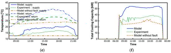
Figure 15.
Total building electricity consumptions of baseline and faulted scenarios: Excessive infiltration through the building envelope. (a) baseline: return/supply temperatures; (b) baseline: total cooling capacity; (c) damper 50% open: return/supply temperatures; (d) damper 50% open: total cooling capacity; (e) damper 100% open: return/supply temperatures; (f) damper 100% open: total cooling capacity.
3.8. Return Air Duct Leakage
The experiments for the baseline and faulted scenarios were conducted with the RTU operating in full load (100% fan power and all VAV dampers fully open). The fault intensity is defined at the full load condition and referenced to the design flow rate. For example, if the supply air design flow rate is 1000 cfm and the fault intensity is 15% leakage, then 150 cfm of the outdoor air is introduced to the air system prior to the conditioning of the air. To impose the fault, the operator inserted an adjustable opening—such as a circular cutout—in the return duct at the RTU, such that a portion of the outdoor air was introduced into the air system. To set up each test, the operator temporarily overrode the building control system to force all VAV dampers to the fully open position and force the RTU to the full load operating condition. The operator then adjusted the size of the opening by adjusting the damper opening to achieve the specified fault intensity. The airflow through the damper was estimated using the measured pressure drop and the value of the damper opening position:
where q = airflow (cfm); = measured pressure drop (in.w.g.); K = constant of proportionality dependent upon orifice area (damper opening position).
The damper opening remained unchanged for the duration of each fault test.
Table 12 presents CV (RMSE) and NMBE results of detailed model outputs for the return air duct leakage fault. The CV (RMSE) results are mostly within the target level (besides latent cooling capacity predictions), whereas total building energy and heating energy predictions are underpredicted compared to measurements, as shown in NMBE results. Although the results of the baseline and 15% leakage scenario show reasonable predictions against measurements, the 30% leakage scenario overpredicts the total cooling capacity.
Table 12.
CV (RMSE) and NMBE Calculations for Detailed Model Outputs: Return Air Duct Leakage.
Figure 16 shows detailed plots, including total cooling capacity (total cooling capacity uncertainty ≈ 3% of reading) and total VAV heating (sensor accuracy = ±0.5% of reading) predictions for all scenarios. The difference in the transient response because of thermal and mechanical delay between measurements and simulation is seen in both cooling capacity and VAV heating results. The predicted cooling capacity peak is much higher than the measured value, and the VAV reheat peak timings occur earlier in the model. The total cooling capacity predictions of the baseline and 15% leakage scenario show reasonable agreement with measurements, but the 30% leakage scenario significantly overpredicts the cooling capacity. The fault model applies the air leakage by increasing the fraction of the outdoor air linearly based on the fault intensity definition; thus, the load on the cooling coil also increases linearly based on the amount of outdoor air introduced. However, as with the results shown in the economizer damper stuck fault, comparisons between measurements and the unfaulted simulations show that the impact of the outdoor air introduced into the return air system is also nonlinear. Thus, this model also requires an improvement for capturing nonlinearities of the duct leakage in the air system.

Figure 16.
Total heating and cooling energy consumptions of baseline and faulted scenarios: Return air duct leakage. (a) baseline: total cooling capacity; (b) baseline: heating energy consumption; (c) +15% leak in return air duct: total cooling capacity; (d) +15% leak in return air duct: heating energy consumption; (e) +30% leak in return air duct: total cooling capacity; (f) +30% leak in return air duct: heating energy consumption.
4. Discussion, Limitations, and Future Work
As demonstrated by the quantitative and qualitative validation in Section 3, the fault models’ validation results varied depending on characteristics of the fault and model structure. Faults such as HVAC/lighting setback error, thermostat measurement bias, and excessive infiltration where existing EnergyPlus variables were modified captured relative impacts (e.g., increased heating or cooling demand) correctly in the building system. However, these fault models require a more accurate building model in order to predict individual room behaviors (e.g., room temperature, VAV heating output) precisely. Although the nonstandard refrigerant charging model provided reasonable predictions compared to measurements for all faulted scenarios, the condenser fouling fault model (which has the same model structure of the nonstandard refrigerant charging) mostly underpredicted the degradation impacts. We also identified opportunities for model improvements for the stuck economizer damper opening and return air duct leakage fault models, where measurements showed nonlinear behavior that is not present in the model. Following are summaries of limitations that can lead to future work:
- -
- In order to precisely estimate the impacts of faults on the building, and especially for fault models that only modify existing variables in EnergyPlus, the building model requires a more rigorous calibration process to precisely reflect the thermal behavior of the building. Although poor humidity level prediction in the building model did not have a significant impact on the building’s overall performance (because the absolute scale of the latent load was already small), the difference in the rate of temperature decay during the unoccupied hours did lead to significant overprediction of heating energy consumption for the winter season simulation.
- -
- Fault models for predicting the degradation of the RTU performance (e.g., condenser fouling and nonstandard refrigerant charging) were developed by estimating the relative deviation from the nominal equipment’s performance. Although the nonstandard refrigerant charging model showed good agreement against measurements, the condenser fouling model requires additional improvement based on validation results. Additionally, a more accurate DX unit model (or cooling coil model in EnergyPlus) is necessary to accurately estimate both sensible and latent cooling performances of the unit.
- -
- The stuck economizer damper and return air duct leakage faults are modeled by linearly introducing the outdoor air into the air system depending on the definition of the fault intensity. However, measurements showed that the impacts from a stuck damper and return air duct leakage are nonlinear. While pressure-based airflow network models can be used for improved prediction of outdoor air introduced into the air system, this type of model typically requires high computational requirements that are not suitable in building energy simulation tools. Thus, these two fault models also need improvements for capturing nonlinearities.
5. Conclusions
This work was motivated by the need for development of a cost-effective AFDD tool for the small commercial buildings market, where the energy savings potential is high but the return of the AFDD tool investment is low. In this study, the objective was to use a building energy simulation tool suite (EnergyPlus and OpenStudio) to generate a data set that can be used for training an AFDD algorithm. Because there has not been a study for developing and validating models to simulate faults that are common in small commercial buildings, Part I of this article series presented a library of fault models, including detailed descriptions of each fault model structure and implementation within EnergyPlus.
In this article (Part II), we presented a methodology of validating fault models with OpenStudio as well as validation results against measurements from a reference building. We conducted experiments and simulations for eight different faults (a total of 39 different baseline and faulted scenarios) using the reference building and fault models in order to enable model validations. The experimental results were uploaded in a public repository for future use cases [45]. Out of eight fault models validated in this study, five fault models (HVAC setback error, lighting setback error, thermostat measurement bias, excessive infiltration, and nonstandard refrigerant charging) showed reasonable predictions against measurements (assuming adequate accuracy of reference building model), and three fault models (condenser fouling, economizer opening stuck, and return air duct leakage) were identified as needing improvement.
Author Contributions
Conceptualization, J.K., J.E.B. and S.F.; methodology, J.K., J.E.B. and S.F.; software, J.K. and D.G.; formal analysis, J.K.; investigation, J.K. and P.I.; resources, D.G. and P.I.; data curation, J.K.; writing—original draft preparation, J.K., J.E.B. and S.F.; writing—review and editing, J.K., J.E.B., S.F., M.L., P.I.; visualization, J.K.; supervision, J.E.B., S.F. and M.L.; project administration, J.E.B., S.F. and M.L.; funding acquisition, J.E.B. and S.F.
Funding
This work was authored in part by the National Renewable Energy Laboratory, operated by Alliance for Sustainable Energy, LLC, for the U.S. Department of Energy (DOE) under Contract No. DE-AC36-08GO28308. Funding was provided by the U.S. Department of Energy Office of Energy Efficiency and Renewable Energy Building Technologies Office. The views expressed in the article do not necessarily represent the views of the DOE or the U.S. Government. The U.S. Government retains and the publisher, by accepting the article for publication, acknowledges that the U.S. Government retains a nonexclusive, paid-up, irrevocable, worldwide license to publish or reproduce the published form of this work, or allows others to do so, for U.S. Government purposes.
Acknowledgments
The authors greatly appreciate the experimental support of Jaewan Joe of Oak Ridge National Laboratory during the last phase of this project.
Conflicts of Interest
The authors declare no conflict of interest.
Nomenclature
| Greek symbols | |
| ∆ | difference in time |
| solar zenith angle, rad | |
| Acronyms | |
| AFDD | automated fault detection and diagnosis |
| C | air leakage coefficient of the airflow power law |
| CFM 50 | airflow measured with a blower door test with 50 pascals, cfm |
| COP | coefficient of performance |
| CV (RMSE) | coefficient of variation of the root-mean-square error, % |
| DHI | diffuse horizontal irradiance, W/m2 |
| DNI | direct normal irradiance, W/m2 |
| DX | direct expansion |
| ELA | effective leakage area, in2 |
| FRP | flexible research platform |
| GHI | global horizontal irradiance, W/m2 |
| HVAC | heating, ventilating, and air conditioning |
| K | constant of proportionality dependent upon orifice area |
| N | pressure exponent of the airflow power law |
| n | total number of data points |
| NMBE | normalized mean bias error, % |
| NSRDB | National Solar Radiation Database |
| PAT | Parametric Analysis Tool |
| P | Pressure, in.w.g. |
| q | airflow, cfm |
| RTU | rooftop unit |
| y | actual metered value |
| predicted value | |
| average of metered value | |
| VAV | variable air volume |
Appendix A
Table A1.
Experimental configurations for all fault experiments.
Table A1.
Experimental configurations for all fault experiments.
| HVAC Setback Error | Scenario | Baseline | 3 h delayed onset | 3 h early termination | No setback | ||||||
| Fault intensity definition | - | Delay in onset of overnight HVAC setback, in hours | Early termination of overnight HVAC setback, in hours | Absence of overnight HVAC setback (binary) | |||||||
| Fault imposition method | - | Modify the control programming to either delay/terminate/remove the setback schedules. | |||||||||
| Tested date | 30/11/2017 | 7-8/8/2018 | 1/12/2017 | 5/8/2018 | 3/12/2017 | 4/8/2018 | 20/12/2017 | 28/8/2018 | |||
| Average daily ambient temperature | 9.0 °C | 26.1 °C | 9.1 °C | 25.7 °C | 10.5 °C | 25.4 °C | 11.6 °C | 26.1 °C | |||
| Exception | - | Fault imposed earlier and removed later than other fault experiments to avoid transient effects during transitions. | |||||||||
| Lighting Setback Error | Scenario | Baseline | 3 h delayed onset | 3 h early termination | No setback | ||||||
| Fault intensity definition | - | Delay in onset of overnight lighting setback, in hours | Early termination of overnight lighting setback, in hours | Absence of overnight HVAC setback (binary) | |||||||
| Fault imposition method | - | Modify the control programming to either delay/terminate/remove the setback schedules. | |||||||||
| Tested date | 5/2/2019 | 7/2/2018 | 9/2/2018 | 18/2/2018 | |||||||
| Average daily ambient temperature | 4.3 °C | 3.1 °C | 1.6 °C | 7.4 °C | |||||||
| Exception | - | Fault imposed earlier and removed later than other fault experiments to avoid transient effects during transitions. | |||||||||
| Condenser Fouling | Scenario | Baseline | 28% fouling | 58% fouling | |||||||
| Fault intensity definition | - | Percent reduction in condenser coil airflow at full load. | |||||||||
| Fault imposition method | - | Cover the condenser face using pretested blocking media. | |||||||||
| Tested date | 2/9/2019 | 27/8/2017 | 29/8/2017 | ||||||||
| Average daily ambient temperature | 16.4 °C | 22.9 °C | 22.1 °C | ||||||||
| Exception | - | RTU operated in full load (supply fan in 100% speed) and all VAV dampers fully open. | |||||||||
| Nonstandard Refrigerant Charging | Scenario | Baseline | 15% undercharge | 30% undercharge | 15% overcharge | ||||||
| Fault intensity definition | - | Fraction of refrigerant charge level deviated from normal charge. | |||||||||
| Fault imposition method | - | Add or remove refrigerant to the refrigerant circuit. | |||||||||
| Tested date | 22-23/8/2019 | 14/8/2018 | 16/8/2018 | 18/8/2018 | |||||||
| Average daily ambient temperature | 23.4 °C | 24.1 °C | 24.4 °C | 24.8 °C | |||||||
| Exception | - | No exception. Based on normal operating conditions and schedule. | |||||||||
| Thermostat Measurement Bias | Scenario | Baseline | −2.2 °C bias in room 105 and 205 | +2.2 °C bias in room 105 and 205 | −2.2 °C bias in room 105, 205, 106, and 206 | +2.2 °C bias in room 105, 205, 106, and 206 | |||||
| Fault intensity definition | - | Zone thermostat measurement deviation from correct value in °C (e.g., positive fault intensity = measurement reading higher than actual). | |||||||||
| Fault imposition method | - | Adjust temperature setpoints of rooms by a number of degrees equal in magnitude and opposite in sign to the fault intensity. | |||||||||
| Tested date | 9/8/2019 | 10/8/2019 | 14/8/2019 | 12/8/2019 | 13/8/2019 | ||||||
| Average daily ambient temperature | 26.0 °C | 26.6 °C | 25.7 °C | 25.5 °C | 26.6 °C | ||||||
| Exception | - | No exception. Based on normal operating condition and schedule. | |||||||||
| Excessive Infiltration Through the Building Envelope | Scenario | Baseline | +20% infiltration | +40% infiltration | |||||||
| Fault intensity definition | - | Effective infiltration area as a percentage of the nominal value. | |||||||||
| Fault imposition method | - | Open windows to achieve target infiltration area. | |||||||||
| Tested date | 9-10/12/2019 | 7/12/2017 | 14/12/2017 | ||||||||
| Average daily ambient temperature | 1.2 °C | 3.8 °C | 0.6 °C | ||||||||
| Exception | - | Baseline and fault tests conducted only when daily average ambient temperature was less than 7.2 °C in order to increase the fault impact. | |||||||||
| Economizer Opening Stuck at a Fixed Position | Scenario | Baseline | Damper 50% open | Damper 100% open | |||||||
| Fault intensity definition | - | Ratio of economizer damper at the stuck position (0 = fully closed, 1 = fully open). | |||||||||
| Fault imposition method | - | Modify the control programming to override the position of the outdoor air damper. | |||||||||
| Tested date | 20/8/2019 | 15/8/2019 | 19/8/2019 | ||||||||
| Average daily ambient temperature | 27.4 °C | 25.4 °C | 26.4 °C | ||||||||
| Exception | - | No exception. Based on normal operating condition and schedule. | |||||||||
| Return Air Duct Leakage | Scenario | Baseline | 15% return duct leakage | 30% return duct leakage | |||||||
| Fault intensity definition | - | Unconditioned air introduced into the return air stream at full load condition as a percent of the design airflow rate. | |||||||||
| Fault imposition method | - | Insert an adjustable opening in the return duct at the RTU and adjust this to achieve the target air-leakage rate. | |||||||||
| Tested date | 21-22/6/2019 | 15/6/2018 | 19/6/2018 | ||||||||
| Average daily ambient temperature | 24.1 °C | 25.6 °C | 27.4 °C | ||||||||
| Exception | - | RTU operated under full load (supply fan at 100% speed) and all VAV dampers fully open. | |||||||||
References
- Kim, J.; Frank, S.; Braun, J.E.; Goldwasser, D. Representing small commercial building faults in energyplus, Part I: Model development. Buildings 2019, 9, 233. [Google Scholar] [CrossRef]
- Kim, J.; Cai, J.; Braun, J.E. Common Faults and Their Prioritization in Small Commercial Buildings; Common Faults and Their Prioritization in Small Commercial Buildings: February 2017–December 2017. 2018. Available online: https://www.nrel.gov/docs/fy18osti/70136.pdf (accessed on 12 November 2019).
- Roth, K.W.; Westphalen, D.; Feng, M.Y.; Llana, P.; Quartararo, L. Energy Impact of Commercial Building Controls and Performance Diagnostics: Market Characterization, Energy Impact of Building Faults and Energy Savings Potential; Building Technologies Program; National Technical Reports Library: Washington, DC, USA, 2005. [Google Scholar]
- Frank, S.; Heaney, M.; Jin, X.; Robertson, J.; Cheung, H.; Elmore, R.; Henze, G. Hybrid Model-Based and Data-Driven Fault Detection and Diagnostics for Commercial Buildings; American Council for an Energy-Efficient Economy (ACEEE): Washington, DC, USA, 2016. [Google Scholar]
- Kim, W.; Katipamula, S. A review of fault detection and diagnostics methods for building systems. Sci. Technol. Built Environ. 2018, 24, 3–21. [Google Scholar] [CrossRef]
- Yu, Y.; Yuill, D.; Behfar, A. Fault Detection and Diagnostics (FDD) Methods for Supermarkets-Phase 1; ASHRAE: Omaha, NE, USA, 2017. [Google Scholar]
- Yuill, D.P.; Braun, J.E. Evaluating the performance of fault detection and diagnostics protocols applied to air-cooled unitary air-conditioning equipment. HVAC&R Res. 2013, 19, 882–891. [Google Scholar]
- Yuill, D.P.; Braun, J.E. Effect of the distribution of faults and operating conditions on AFDD performance evaluations. Appl. Therm. Eng. 2016, 106, 1329–1336. [Google Scholar] [CrossRef]
- Ali, A.H.H.; Ismail, I.M. Evaporator air-side fouling: Effect on performance of room air conditioners and impact on indoor air quality. HVAC&R Res. 2008, 14, 209–219. [Google Scholar]
- Aydin, C.; Ozerdem, B. Air leakage measurement and analysis in duct systems. Energy Build. 2006, 38, 207–213. [Google Scholar] [CrossRef][Green Version]
- Bell, I.H.; Groll, E.A. Air-side particulate fouling of microchannel heat exchangers: Experimental comparison of air-side pressure drop and heat transfer with plate-fin heat exchanger. Appl. Therm. Eng. 2011, 31, 742–749. [Google Scholar] [CrossRef]
- Cho, S.-H.; Yang, H.-C.; Zaheer-uddin, M.; Ahn, B.-C. Transient pattern analysis for fault detection and diagnosis of HVAC systems. Energy Convers. Manag. 2005, 46, 3103–3116. [Google Scholar] [CrossRef]
- Comstock, M.C.; Braun, J.E.; Groll, E.A. The sensitivity of chiller performance to common faults. HVAC&R Res. 2001, 7, 263–279. [Google Scholar]
- Goswami, D.Y.; Ek, G.; Leung, M.; Jotshi, C.K.; Sherif, S.A.; Colacino, F. Effect of refrigerant charge on the performance of air-conditioning systems. In Proceedings of the IECEC-97 Proceedings of the Thirty-Second Intersociety Energy Conversion Engineering Conference (Cat. No.97CH6203), Honolulu, HI, USA, 27 July–1 August 1997; Volume 3, pp. 1635–1640. [Google Scholar]
- Kim, M.; Payne, W.V.; Domanski, P.A.; Yoon, S.H.; Hermes, C.J.L. Performance of a residential heat pump operating in the cooling mode with single faults imposed. Appl. Therm. Eng. 2009, 29, 770–778. [Google Scholar] [CrossRef]
- Kim, W.; Braun, J.E. Evaluation of the impacts of refrigerant charge on air conditioner and heat pump performance. Int. J. Refrig. 2012, 35, 1805–1814. [Google Scholar] [CrossRef]
- Mukhopadhyaya, P.; Bomberg, M.; Kumaran, M.K.; Drouin, M.; Lackey, J.C.; Van Reenen, D.; Normandin, N. Long-term thermal resistance of polyisocyanurate foam insulation with gas barrier. In Proceedings of the IX International Conference on Performance of Exterior Envelopes of Whole Buildings, Clearwater Beach, FL, USA, 5–10 December 2004. [Google Scholar]
- O’Neal, D.L.; Farzad, M. The effect of improper refrigerant charging on the performance of an air conditioner with capillary tube expansion. Energy Build. 1990, 14, 363–371. [Google Scholar] [CrossRef]
- Pak, B.C.; Groll, E.A.; Braun, J.E. Impact of fouling and cleaning on plate fin and spine fin heat exchanger performance. ASHRAE Trans. 2005, 111, 496–504. [Google Scholar] [CrossRef]
- Palmiter, L.; Kim, J.-H.; Larson, B.; Francisco, P.W.; Groll, E.A.; Braun, J.E. Measured effect of airflow and refrigerant charge on the seasonal performance of an air-source heat pump using R-410A. Energy Build. 2011, 43, 1802–1810. [Google Scholar] [CrossRef]
- Qureshi, B.A.; Zubair, S.M. The impact of fouling on the condenser of a vapor compression refrigeration system: An experimental observation. Int. J. Refrig. 2014, 38, 260–266. [Google Scholar] [CrossRef]
- Rice, C.K. The Effect of Void Fraction Correlation and Heat Flux Assumption on Refrigerant Charge Inventory Predictions; Oak Ridge National Lab.: Oak Ridge, TN, USA, 1987. [Google Scholar]
- Siegel, J.A.; Nazaroff, W.W. Predicting particle deposition on HVAC heat exchangers. Atmos. Environ. 2003, 37, 5587–5596. [Google Scholar] [CrossRef]
- Simmler, H.; Brunner, S. Vacuum insulation panels for building application: Basic properties, aging mechanisms and service life. Energy Build. 2005, 37, 1122–1131. [Google Scholar] [CrossRef]
- Wallace, L.A.; Emmerich, S.J.; Howard-Reed, C. Continuous measurements of air change rates in an occupied house for 1 year: The effect of temperature, wind, fans, and windows. J. Expo. Anal. Environ. Epidemiol. Princet. 2002, 12, 296–306. [Google Scholar] [CrossRef]
- Wichman, A.; Braun, J. Fault detection and diagnostics for commercial coolers and freezers. HVAC&R Res. 2008, 15:1, 77–99. [Google Scholar] [CrossRef]
- Woradechjumroen, D.; Yu, Y.; Li, H.; Yu, D.; Yang, H. Analysis of HVAC system oversizing in commercial buildings through field measurements. Energy Build. 2014, 69, 131–143. [Google Scholar] [CrossRef]
- Zirkelbach, D.; Schafaczek, B.; Künzel, H.M. Thermal performance degradation of foam insulation in inverted roofs due to moisture accumulation. In Proceedings of the XII DBMC 2011, 12th International Conference on Durability of Building Materials and Components, Porto, Portugal, 12–15 April 2011; Volume 1, pp. 529–536. [Google Scholar]
- Cheung, H.; Braun, J.E. Simulation of fault impacts for vapor compression systems by inverse modeling. Part I: Component modeling and validation. HVAC&R Res. 2013, 19, 892–906. [Google Scholar]
- Cheung, H.; Braun, J.E. Simulation of fault impacts for vapor compression systems by inverse modeling. Part II: System modeling and validation. HVAC&R Res. 2013, 19, 907–921. [Google Scholar]
- Cheung, H.; Braun, J.E. Empirical modeling of the impacts of faults on water-cooled chiller power consumption for use in building simulation programs. Appl. Therm. Eng. 2016, 99, 756–764. [Google Scholar] [CrossRef]
- Dey, M.; Rana, S.P.; Dudley, S. Smart building creation in large scale HVAC environments through automated fault detection and diagnosis. Future Gener. Comput. Syst. 2018. [Google Scholar] [CrossRef]
- Farzad, M. Modeling the Effects of Refrigerant Charging on Air Conditioner Performance Characteristics for Three Expansion Devices. Ph.D. Thesis, Texas A&M University, College Station, TX, USA, 1990. [Google Scholar]
- Guo, Y.; Tan, Z.; Chen, H.; Li, G.; Wang, J.; Huang, R.; Liu, J.; Ahmad, T. Deep learning-based fault diagnosis of variable refrigerant flow air-conditioning system for building energy saving. Appl. Energy 2018, 225, 732–745. [Google Scholar] [CrossRef]
- Harms, T.M. Charge Inventory System Modeling and Validation for Unitary Air Conditioners. Ph.D. Thesis, Purdue University, West Lafayette, IN, USA, 2002. [Google Scholar]
- Inamdar, H.V.; Groll, E.A.; Weibel, J.A.; Garimella, S.V. Prediction of air-side particulate fouling of HVAC&R heat exchangers. Appl. Therm. Eng. 2016, 104, 720–733. [Google Scholar]
- Li, S.; Wen, J. Application of pattern matching method for detecting faults in air handling unit system. Autom. Constr. 2014, 43, 49–58. [Google Scholar] [CrossRef]
- Reddy, T.A. Application of a generic evaluation methodology to assess four different chiller FDD methods (RP-1275). HVAC&R Res. 2007, 13, 711–729. [Google Scholar]
- Rossi, T.M. Detection, Diagnosis, and Evaluation of Faults in Vapor Compression Equipment. Ph.D. Thesis, Purdue University, West Lafayette, IN, USA, 1995. [Google Scholar]
- Shen, B.; Braun, J.E.; Groll, E.A. Improved methodologies for simulating unitary air conditioners at off-design conditions. Int. J. Refrig. 2009, 32, 1837–1849. [Google Scholar] [CrossRef]
- NREL Open Studio Fault Models. Available online: https://github.com/NREL/OpenStudio-fault-models (accessed on 23 May 2019).
- Cheung, H.; Braun, J.E. Development of Fault Models for Hybrid Fault Detection and Diagnostics Algorithm; National Renewable Energy Laboratory: Golden, CO, USA, 2015. [Google Scholar]
- Im, P.; Bhandari, M.S.; New, J.R. Multiyear Plan for Validation of EnergyPlus Multi-Zone HVAC System Modeling using ORNL’s Flexible Research Platform; Oak Ridge National Lab (ORNL), Building Technologies Research and Integration Center (BTRIC): Oak Ridge, TN, USA, 2016. [Google Scholar]
- Goldwasser, D.; Ball, B.L.; Farthing, A.D.; Frank, S.M.; Im, P. Advances in Calibration of Building Energy Models to Time Series Data: Preprint; National Renewable Energy Lab. (NREL): Golden, CO, USA, 2018. [Google Scholar]
- Kim, J.; Im, P.; Leach, M. Curated Test Fault Data Set. Available online: https://openei.org/doe-opendata/dataset/curated-test-fault-data-set (accessed on 16 November 2019).
- National Renewable Energy Laboratory. OpenStudio. Available online: https://www.openstudio.net/ (accessed on 20 November 2019).
- Goldwasser, D.; Macumber, D.; Parker, A.; Lee, E.; Guglielmetti, R.; Brackney, L. The Life Cycle of an OpenStudio Measure: Development, Testing, Distribution, and Application; National Renewable Energy Lab. (NREL): Golden, CO, USA, 2016. [Google Scholar]
- ASHRAE. ASHRAE Guideline 14-2014—Measurement of Energy, Demand, and Water Savings; American Society of Heating, Refrigerating and Air-Conditioning Engineers, Inc. (ASHRAE): Atlanta, GA, USA, 2014. [Google Scholar]
- National Solar Radiation Database (NSRDB). Available online: https://nsrdb.nrel.gov/ (accessed on 5 September 2019).
- Wheeler, G.; Kozubal, E.; Judkoff, R. Experimental design and laboratory characterization of a medium- and high-efficiency rooftop unit for use in building energy simulations. In Proceedings of the International Refrigeration and Air Conditioning Conference, West Lafayette, Indiana, 9–12 August 2018; Purdue University. [Google Scholar]


© 2019 by the authors. Licensee MDPI, Basel, Switzerland. This article is an open access article distributed under the terms and conditions of the Creative Commons Attribution (CC BY) license (http://creativecommons.org/licenses/by/4.0/).