Probabilistic Seismic Assessment of Existing Masonry Buildings

Abstract

The evaluation of seismic performance of existing masonry buildings is a critical issue in assessing the seismic vulnerability of the built environment. With this aim, non-linear static analysis is commonly used, but results are influenced significantly by the collapse criteria adopted, as well as by the assumptions about material properties and drift capacity of masonry walls. A methodology for the probabilistic assessment of the seismic risk index is proposed by means of an original non-linear pushover type algorithm developed by the authors. The main sources of uncertainties related to masonry parameters and their influence on seismic risk indices are identified by means of sensitivity analysis. Response surfaces for the seismic risk indices are thus defined through general polynomial chaos expansion in order to quantify the uncertainties in the resulting seismic risk index. Finally, a seismic performance classification is presented to help stakeholders to manage risks and define priorities for seismic retrofit. The methodology together with the outcomes is illustrated for a set of existing masonry buildings that are part of the school system in the Municipality of Florence.

1. Introduction

Seismic vulnerability of the built environment has been confirmed and emphasized by the heavy consequences of recent earthquakes. For this reason, the evaluation of seismic performance of existing buildings is increasingly relevant, especially in historical towns characterized by constructions mostly erected without following any specific seismic provisions.

In order to set-up intervention strategies as well as to identify priorities for seismic retrofit and strengthening, also in view of future planning and optimal allocation of available resources in seismic regions, city planners and owners of buildings need a suitable classification of construction in terms of seismic vulnerability. In this context, masonry buildings are topical since they may cover not only relevant and strategic buildings, such as schools, public buildings, hospital facilities and even large industrial buildings, but also include a large part of the architectural heritage to be preserved.

The paper focuses on the development of a probabilistic methodology for the seismic risk assessment and management of existing masonry buildings.

In the framework of an important research project regarding the seismic assessment of more than 80 school masonry buildings in Florence (I), funded by the Municipality of Florence, the authors developed an appropriate methodology in line with the most updated structural codes [1] to classify the seismic performance of masonry buildings, aiming to define priorities in seismic upgrading as well as to identify suitable retrofitting techniques.

Assessment of the seismic performance of existing masonry buildings is the subject of several up to date studies concerning both the modelling strategies and the evaluation of masonry properties. Indeed, understanding and modelling the mechanical behavior of masonry elements is a longstanding challenge in civil engineering [2,3].

Depending on the field of application and the level of complexity, several modeling strategies can be envisaged, like macro-modeling, which is the most common method in engineering practice, simplified micro-modeling, and detailed micro-modeling, where masonry units and mortar are modelled explicitly.

Whatever the approach adopted, in any case results of the assessment are very sensitive to the masonry’s mechanical parameters [4]. Since mechanical parameters of similar masonry typologies can vary in a very wide range; it is not surprising that contrasting conclusions can be derived about the assessment of a given construction simply modifying the assumed values of their relevant mechanical properties. Moreover, despite several “standardized” masonry typologies that can be identified in existing buildings, depending on the material, on the block shape and on its texture, the evaluation of relevant mechanical parameters associated with them is often an open question.

Experimental in situ tests are also limited and characterization of masonry properties is often obtained by visual inspection methods [5] combined with engineering judgment.

A first attempt to consider the uncertainty of masonry properties in the analysis of existing masonry buildings is discussed in [6] where a Bayesian updating procedure is proposed for the calibration of material properties to be used in the structural analysis.

In this study, a method for the analysis of masonry structures is implemented in a probabilistic framework in order to take into account the uncertainties related to the modelling of the shear behavior of masonry walls, aiming to provide a probabilistic assessment of the seismic performance.

Starting from preliminary historical inquiries and in situ tests and surveys, the proposed procedure relies on an ad hoc developed original, reliable and robust, method for the non-linear static seismic analysis of masonry building [7], as summarized in Section 2. Section 3 describes the 11 masonry buildings considered in the present study, while in Section 4 the main sources of uncertainties related to the shear behavior of masonry walls are discussed with special reference to a sensitivity analysis concerning the propagation of uncertainties in the definition of seismic risk index. A probabilistic seismic risk assessment is then proposed leading to the seismic performance classification presented in Section 5.

2. Assessment of the Seismic Performance of Existing Masonry Buildings

The structural assessment of existing buildings and infrastructures requires the preliminary acquisition of all the relevant information regarding the construction and the action that it withstands during its life [8]. Inter alia, to define the actual performance of the construction, particularly significant are data concerning the original configuration and the static scheme of the structure, the sequence of structural modifications, alterations and interventions that occurred during its life, the actual material properties, diagnosis and prognosis of existing crack patterns, failures, settlements extent of degradation and damage.

Focusing on old masonry structures in seismic zones, it must be stressed that they were often built disregarding any seismic design rules and without particularly technical competent workmanship; in Italy, for example, this situation was very common at the end of the 1970s. For this reason, masonry buildings are often highly vulnerable, thereby explaining why they frequently collapse during strong earthquakes.

Furthermore, to estimate the actual performance of existing masonry buildings, specialized methods, based on appropriate mechanical models, should be adopted for their static and seismic analysis.

One of the first methods for the seismic resistance verification of unreinforced masonry building named POR and considering floors infinitely rigid in the horizontal plane, was introduced by Tomažević after the Friuli earthquake in 1976 [9,10]. This method was adopted by the Italian regulations published in 1978 [11] and 1981 [12] for the repair of masonry buildings after earthquake events.

For a consistent assessment of the seismic performance, robust analysis methods but also a proper characterization of the behavior of masonry walls under horizontal loads are needed. Commonly, beside local analyses, non-linear seismic static analyses are performed, supplemented, if necessary, by dynamic linear analyses, mainly devoted to check the order of magnitude of the results. In non-linear static analysis, masonry buildings are mostly modelled by means the so-called equivalent frame model [13], but the resulting structural scheme is usually very complicated and the analysis needs to be “driven” step by step in order to obtain reliable results.

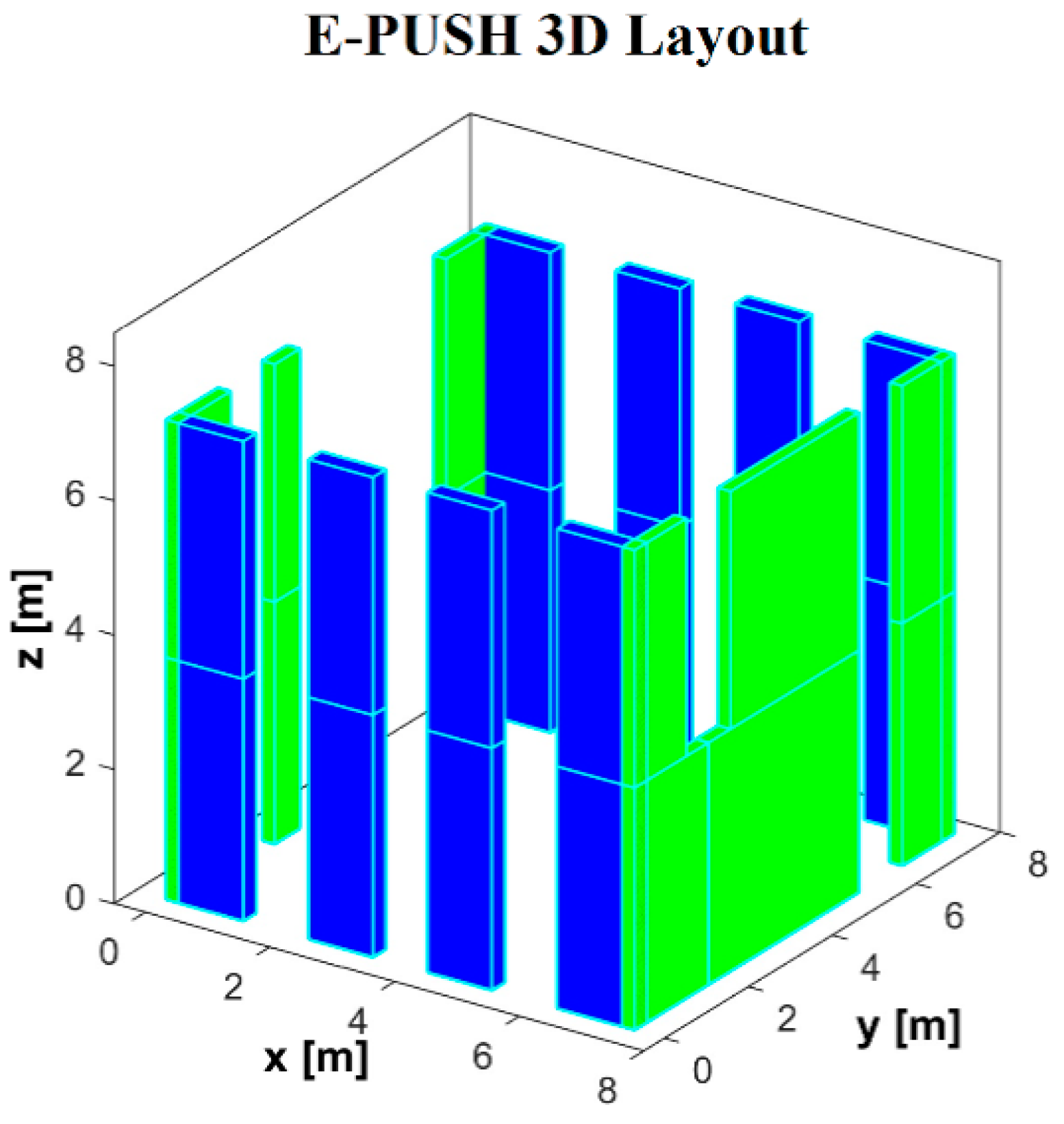
2.1. The E-PUSH Program

As already said, an original method for non-linear static seismic analysis of mono or multi-story buildings masonry building has been developed by the authors and is presented in [7]. The method, which allows taking into account the ductility of the whole structure, recovers some basic assumptions of the classical POR method, but without its limitations and inaccuracies. In addition, the so called E-PUSH software program requires very simple structural models, so that, by contrast with commercial pushover programs, the input results in being extremely robust and nearly independent of the user. As usual, floors are considered, in turn, “flexible” or “rigid”, setting their in-plane stiffness to zero or infinity, respectively, according its deformations in the horizontal plane.

Basic assumptions of the method are:

• only lateral stiffness of masonry walls is taken into account, disregarding transverse stiffness;
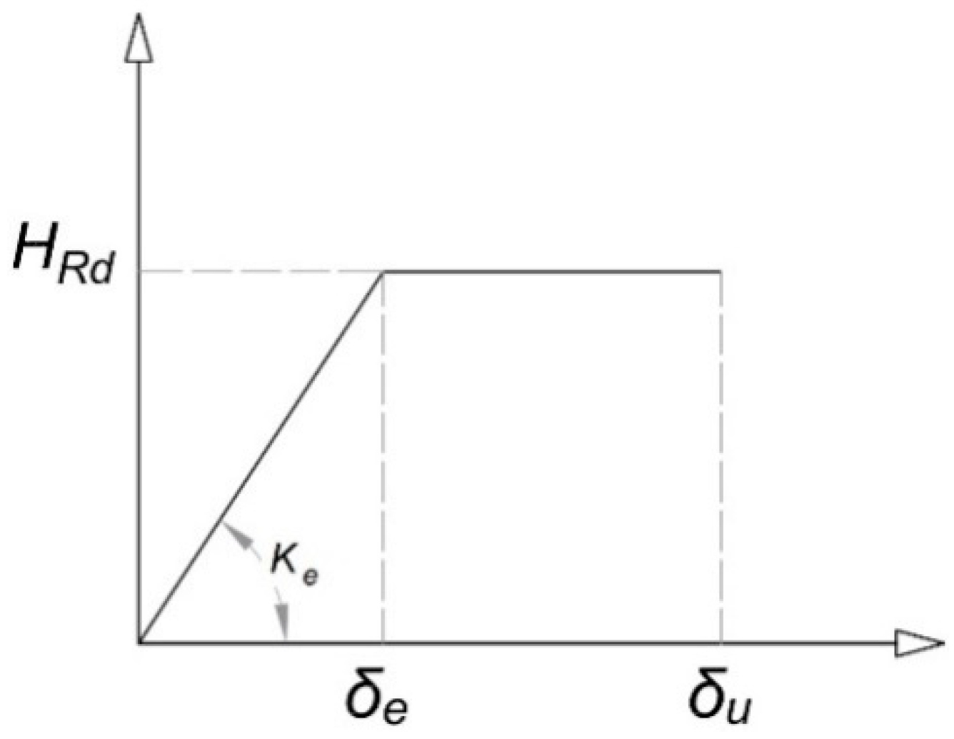
• horizontal force-lateral displacement diagram of the wall is elastic-plastic, with the plastic plateau limited by the elastic drift ${\delta }_e$ and the ultimate drift ${\delta }_u$.
• verification is performed in terms of seismic capacity and demand using the acceleration-displacement response spectra (ADRS) taking into account the story displacements.

The step by step procedure considers increasing values of the given horizontal forces, which are distributed in the plan layout to the resistant shear walls according their stiffness. In short, at each step of the procedure, the inter-story displacement $\delta$ of each shear wall is evaluated and three alternative conditions are checked:

• $\delta <{\delta }_e$, the wall is still in the elastic range;
• ${\delta }_e\le \delta \le {\delta }_u$, the wall is in the plastic range, it achieved its shear force resistance and its equivalent stiffness is reduced;
• $\delta >{\delta }_u$, the wall sustains only vertical loads and its shear resistance and its lateral stiffness are set to zero.

The lateral forces are increased until the base shear resistance reduces to about 80% of the relative maximum base shear resistance or when there is the collapse of all the walls pertaining to a same floor, defining in this way the capacity curve of the whole structure.

The verification procedure, which follows the classical steps of a pushover analysis, is based on the so-called N2 method developed by the University of Ljubljana, described in [14]. The N2 method combines the non-linear static analysis of the multi-degree of freedom model with the response spectrum analysis of an equivalent single degree of freedom system and in the proposed procedure has been implemented according to the following steps:

• the non-linear capacity curve of the structure is transformed in an equivalent bi-linear elastic-plastic curve as described in [14]; the curve is characterized by the maximum force $F_{y,eq}$, calculated averaging the maximum base shear in the non-linear capacity curve and the base shear corresponding to the attainment of the elastic limit; by the yield displacement ${\delta }_{y,eq}$, evaluated as the ratio between $F_{y,eq}$ and the effective stiffness of the structure $K_E$; and by the ultimate displacement ${\delta }_{u,eq}$ which is the maximum displacement in the capacity curve;
• the bi-linear, force-displacement capacity curve, $F-\delta$, of the multi-degree of freedom (MDOF) system is converted in an acceleration-displacement, $S_a-S_d$, capacity diagram, for an equivalent single degree of freedom (SDOF) system, according to the following formulae

  $$S_a=\frac{F}{\mathsf{\Gamma }{m}^{*}};S_d=\frac{\delta }{\mathsf{\Gamma }};$$

  (1)

  where Γ is the mass participation factor given by

  $$\mathsf{\Gamma }=\frac{{{\displaystyle \sum }}_{j=1}^N{m}_j{\varphi }_j}{{{\displaystyle \sum }}_{j=1}^N{m}_j{{\varphi }_j}^2}$$

  (2)

  and $m^{*}$ is the mass of the equivalent SDOF system.

  $$m^{*}={\displaystyle \sum }_{j=1}^N{m}_j{\varphi }_j,$$

  (3)

In Equation (3) $m_j$ are the story masses and ${\varphi }_j$ are the normalized displacements in the considered direction. The elastic period $T^{*}$ of the idealized bi-linear system is thus determined as:

$$T^{*}=2\pi \sqrt{\frac{m^{*}{S}_{d,y}}{S_{a,y}}}$$

(4)

where $S_{d,y}$ is the yield displacement and $S_{a,y}$ is the corresponding acceleration.

3.

in order to obtain the demand diagram, the elastic design spectrum defined in the Italian Building code [15] from the standard pseudo acceleration-natural period, $S_{ae}-T$ is converted into the pseudo acceleration-displacement format $S_{ae}-S_{de}$ through:

$$S_{de}=\frac{T^2}{4{\pi }^2}{S}_{ae};$$

(5)

4.

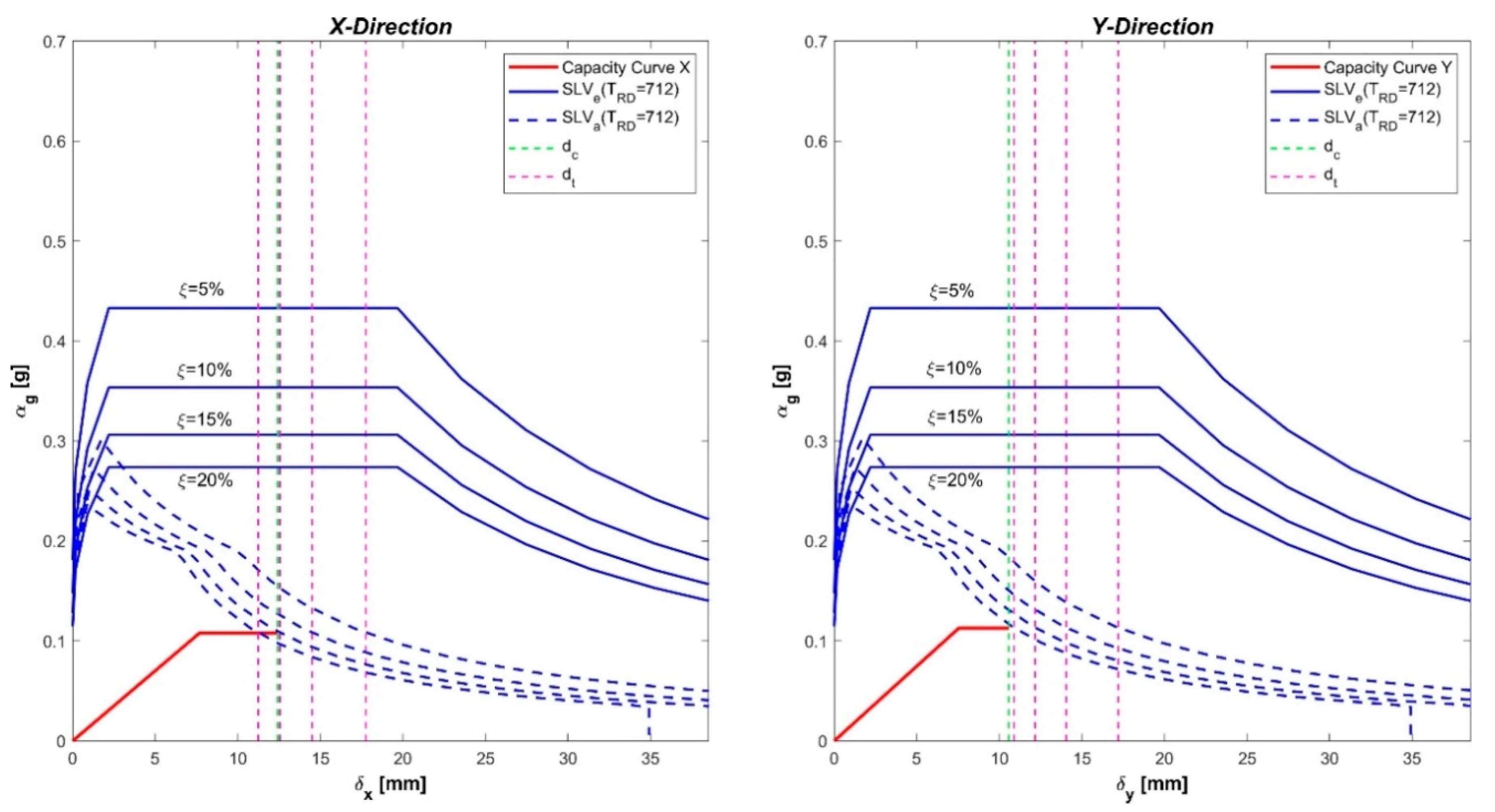
the capacity spectrum and demand spectrum curves are plotted in the same graph, to define displacement demand. If the capacity curve intersects the demand curve, the displacement demand is assumed equal to the intersection point $d_t$. Otherwise, the displacement demand is determined starting from the intersection of the radial line corresponding to the elastic period $T^{*}$ of the structure with the elastic design spectrum defining the acceleration demand $S_{ae}\left(T^{*}\right)$. A reduction factor $R_{\mu }$ is defined as the ratio between the acceleration demand $S_{ae}\left(T^{*}\right)$ and the yield acceleration S_a,y.

$$R_{\mu }=\frac{S_{ae}\left(T^{*}\right)}{S_{a,y}}.$$

(6)

Said $T_C$ the characteristic period of the ground motion, if $T^{*}\ge T_C$ the ductility demand $\mu$, defined as the ratio between the displacement demand and the yield displacement, $\mu =d_t/S_{d,y}$, is equal to $R_{\mu }$, so that

$$d_t=S_{de}\left(T^{*}\right);\mu =R_{\mu }{T}^{*}\ge T_C;$$

(7)

if instead $T^{*}<T_C$, the ductility demand $\mu$ and the displacement demand $d_t$ are calculated according to the formulas given in [10]:

$$\begin{gathered} \mu = \\ (R_{\mu }-1)\frac{T_C}{T^{*}}+1;d_t=\frac{S_{de}\left(T^{*}\right)}{R_{\mu }}(1+(R_{\mu }-1)\frac{T_C}{T^{*}});T^{*}<T_C; \end{gathered}$$

(8)

5.

the seismic performance of the structure is evaluated comparing the displacement demand $d_t$ with the ultimate displacement defined by the capacity curve $d_c$.

The procedure is iterated for different reference period of the seismic demand until it results $d_t$$=d_c$, finally allowing the evaluation of the seismic risk index $I_R$ of the structure,

$$I_R=\frac{PG{A}_C}{PG{A}_D},$$

(9)

where $PG{A}_C$ is the peak ground acceleration resisted by the structure, i.e., when $d_t=d_c,$ and $PG{A}_D$ the design peak ground acceleration provided by the Italian Building Code [15].

An example of the output of the proposed procedure in terms of ADRS for the two relevant directions of the seismic force is reported in Figure 1, referring to one of the school masonry buildings in Florence, described in the following.

The curves in Figure 1, derived from the E-PUSH output for the given case study, include:

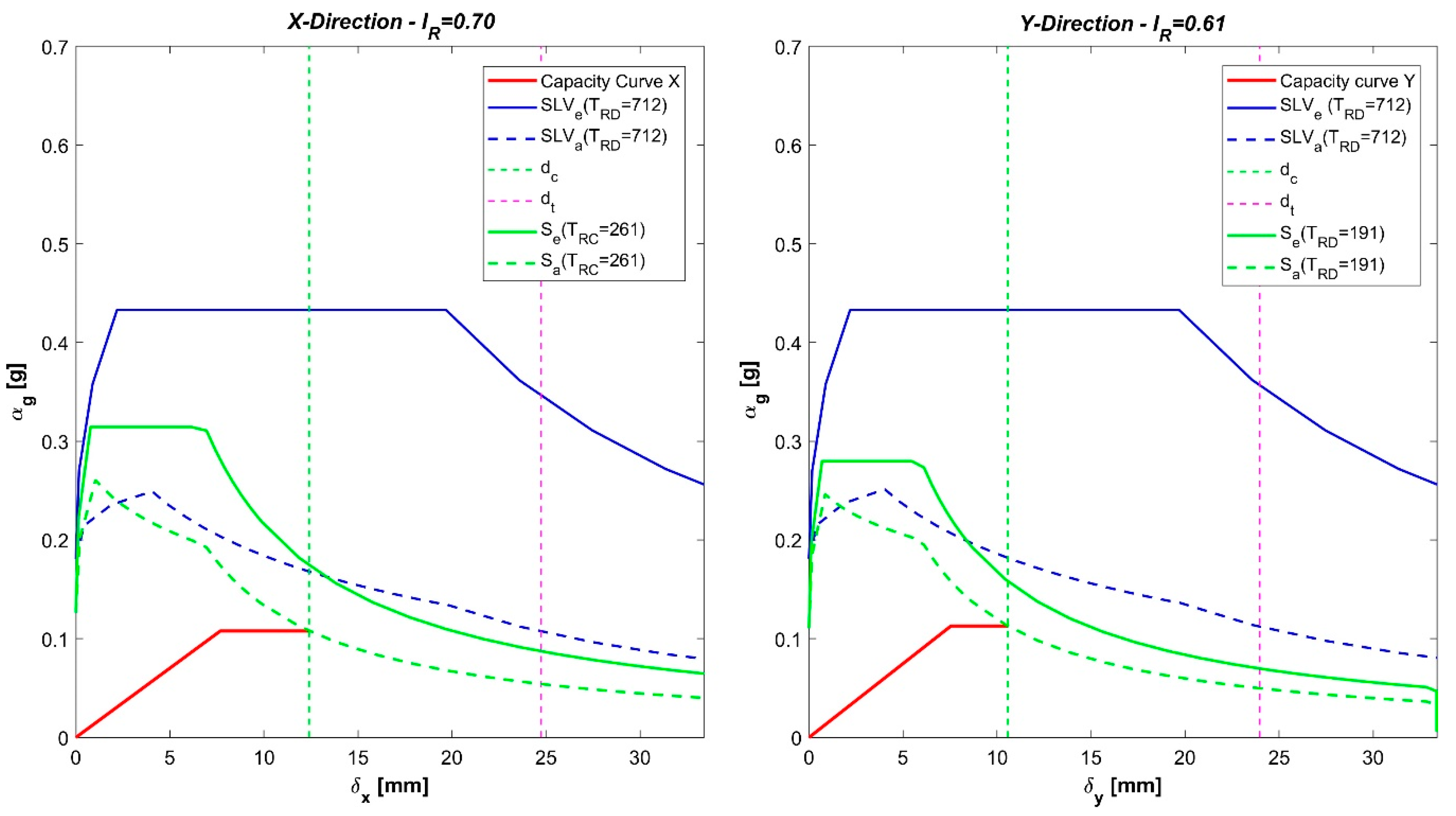
• the bi-linear capacity curve of the structure (red solid line);
• the design spectrum $SL{V}_e$ (blue solid curve) for a return period of 712 years ($T_{RD}$), referring to the ultimate limit state for life safety ($SLV$) of occupants in a given location (Florence Municipality in this case);
• the design inelastic spectrum $SL{V}_a$ (blue dashed curve);
• the displacement demand $d_t$ (scarlet dashed line) to be compared with the ultimate displacement $d_c$ (green dashed line);
• the elastic spectrum (green solid curve) for the return period T_RC consistent with the capacity of the structure ($d_t=d_c$) and the corresponding inelastic spectrum (green dashed curve).

The inelastic spectra obtained with the N2 method are based on the commonly adopted “equal displacement rule” for structures in the medium and long period range, $T^{*}\ge T_C$, and on the procedure proposed by Vidic et al. [16] for the short period structures. The equal displacement rule has been used quite successfully for many years [14] and many statistical studies [16,17,18] have confirmed its applicability in case of structures on firm site, characterized by an average shear wave velocity greater than 180 m/s, with fundamental period in the medium and long period range. For structures characterized by lower fundamental period, the equal displacement rule does not work and $R_{\mu }<\mu$. Formulae for $R_{\mu }$ were calibrated by Vidic et al. in [16] based on a statistical study, and then adopted in the N2 method, assuming the transition period equal to $T_C$, thereby disregarding its dependency on the ductility $\mu$. Anyhow, in case the ductility demand is $\mu <4$ this simplified assumption leads to conservative results.

The influence of the mathematical model adopted for damping and the level of damping ratio in the definition of the $R_{\mu }$ factor has been investigated by Vidic et al. in [16]. It is shown that $R_{\mu }$ increases with decreasing damping coefficient; for example, when $\xi$ decreases from $5\%$ to $2\%$, $R_{\mu }$ increases of about 10% considering the mass-proportional model and of about 20% for instantaneous-stiffness-proportional damping. Consequently, when $\xi <5\%$, adoption of $R_{\mu }$ factor corresponding to 5% damping is safe-sided.

In structural codes the response spectra are usually based on a conventional value $\xi =5\%$ of the viscous damping ratio; damping effects, if any, are taken into account suitably scaling the response spectrum. In the already cited Italian Building Code [15], in agreement with corresponding clauses of Eurocode 8, EN1998-1 [19], the damping correction factor $\eta$ as a function of $\xi$ is given by:

$$\eta =\max \left(\sqrt{\frac{10}{\left(5+\xi \right)}};0.55\right).$$

(10)

Under earthquake excitations, damping increases as the level of damage increases and values of $\xi$ up to 10% to 20% can be reached as discussed in [20].

To analyze the effects of varying viscous damping coefficients on the seismic risk index, a parametric investigation has been carried out for the given case study. In the sensitivity analysis, the response spectra, evaluated according the Italian Building Code, have been modified by varying $\xi$ in the range 5% to 20% by 2.5% steps. The results of the sensitivity study are diagrammatically illustrated in Figure 2 and Figure 3, for the two relevant directions, $x$ and $y$, of the seismic excitation. More precisely, Figure 2, analogous to Figure 1, synthetizes in the ADRS plane results for different values of the viscous damping coefficient $\xi$ ($\xi =5\%$; $\xi =10\%$; $\xi =15\%$; $\xi =20\%$), while Figure 3 shows the variation of seismic risk indexes as a function of the viscous damping coefficient $\xi$. In the case of $\xi =5\%$, the outputs in Figure 2 and Figure 3 obviously correspond to those already illustrated in Figure 1.

Figure 3 also indicates the correction factors $\eta$ obtained introducing in Equation (10) the effective viscous damping coefficients ${\xi }_e$ calculated according the formulation proposed in [20]:

$${\xi }_e=5+\frac{100}{\pi }\left(1-\frac{{\delta }_y}{{\delta }_u}\right),$$

(11)

where ${\delta }_y$ is the displacement of the structure at the first crack and ${\delta }_u$ its ultimate displacement.

Evidently, according to Equation (11), ${\xi }_e$ values can be different in the two directions, like in the present case study, where ${\xi }_{e,x}\approx 17.1\%$ and ${\xi }_{e,y}\approx 14.1\%$, so that also correction factors are different in the two directions. In the present case, Equation (10) provides $\eta \approx 0.67$ in the $x$ direction and $\eta =0.72$ in the $y$ direction.

As expected, the seismic demands are reduced and a significant increase in seismic risk indexes is obtained considering the reduced damping correction factors $\eta$: in fact, the seismic risk index in the $x$ direction becomes bigger than one, increasing by about 46%; while in the $y$ direction it increases by about 41%.

It must be considered that such high values of the damping coefficients correspond to heavy damages of the masonry walls: most likely, they can be achieved by modern brick masonry walls characterized by high ductility, but for historical or ancient masonry walls, the assumption of such high values of damping should be adequately justified.

An analytical alternative formulations of damping coefficient is provided, for example, in [21] where, on the basis of some experimental results, ${\xi }_e$ is expressed as a function of the ductility $\mu$ by:

$${\xi }_e=5+32\frac{\mu -1}{\pi \mu }.$$

(12)

Assuming a ductility factor µ equal to 1.5, as recommended for unreinforced masonry in the guidelines for the application of the POR method [12], in the case study, Equation (12) leads to an equivalent damping of ${\xi }_e\approx 8.4\%$. This damping value, leading to a correction factor $\eta \approx 0.86$, appears to be more consistent with the actual behavior of historical masonry and leads to results in terms of seismic performance more in line with the usual conservative assumption ${\xi }_e=5\%$ (see dashed green line in Figure 3). In this case, the increment of the seismic risk index is about 14.8% in the $x$ direction and about 15.3% in the $y$ direction.

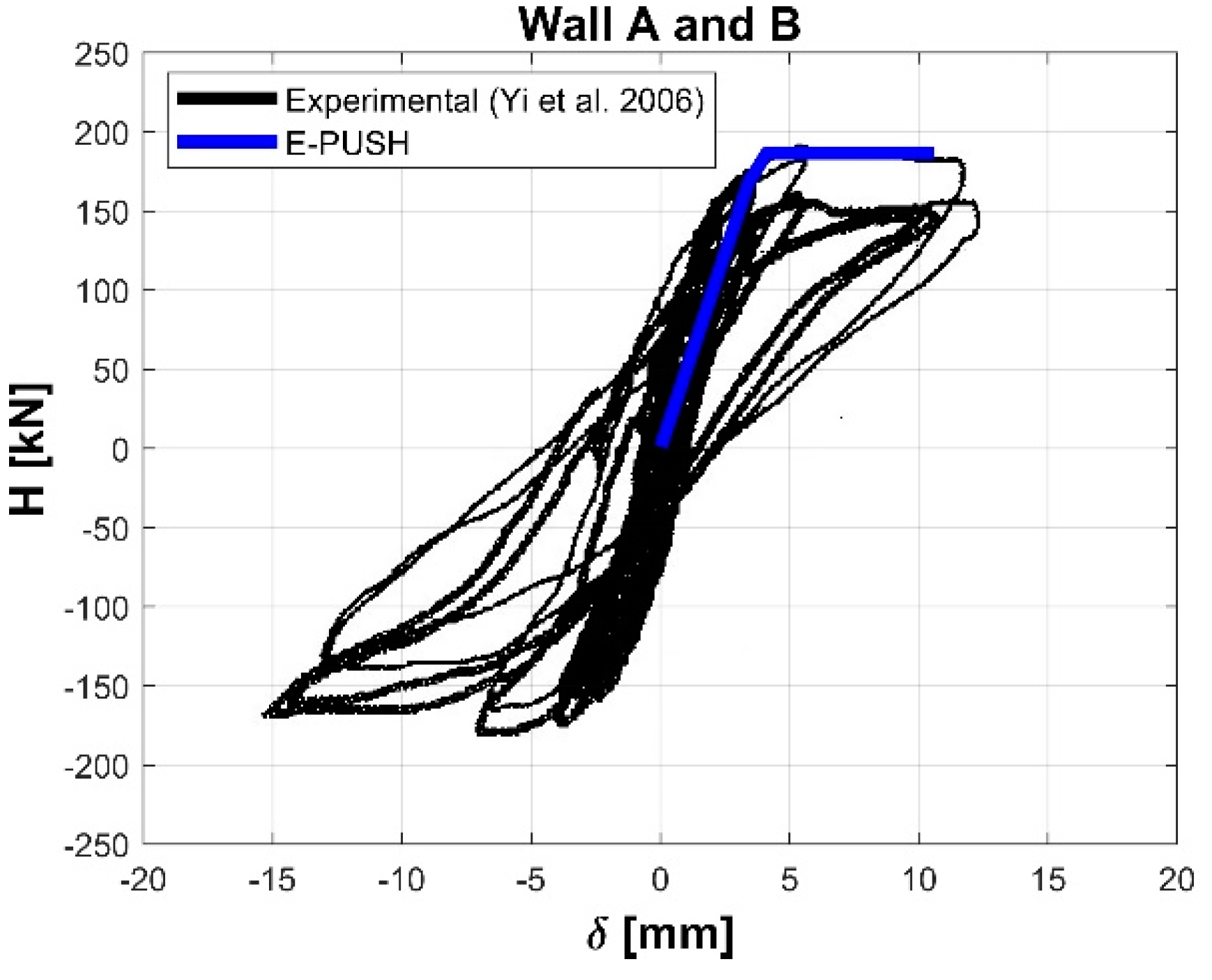
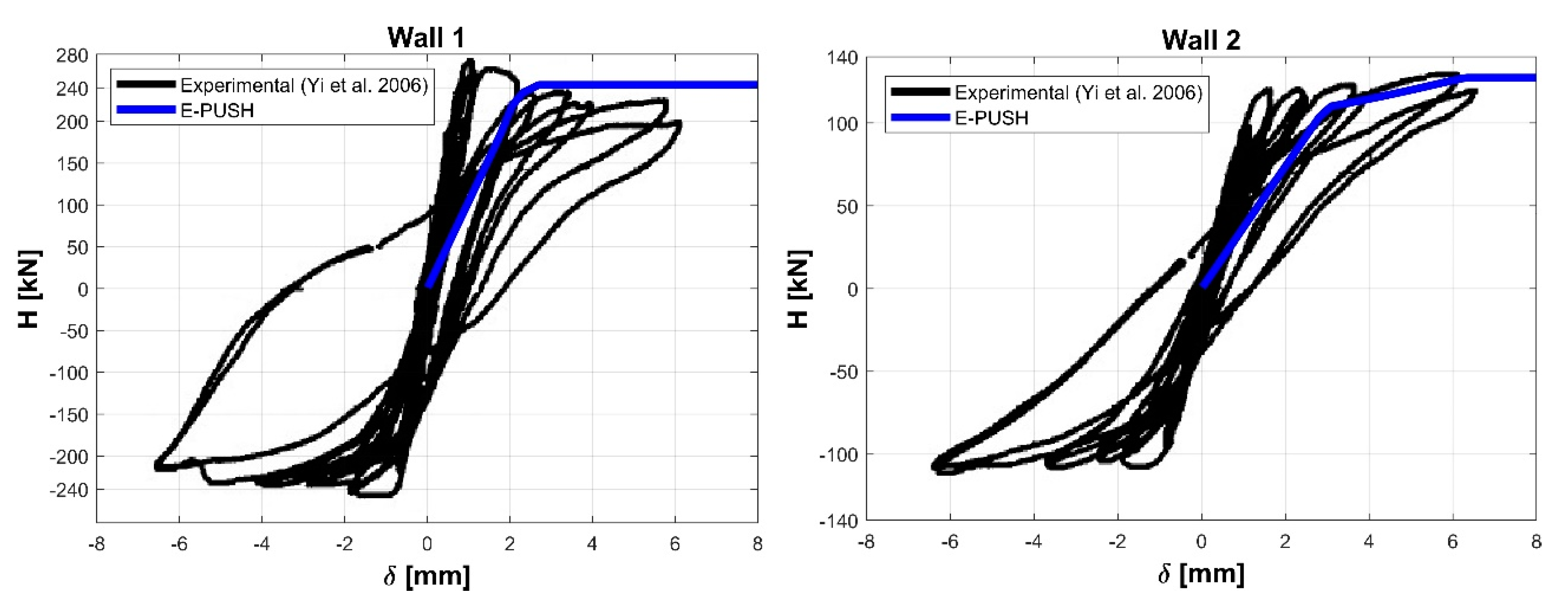
2.2. Validation of the E-PUSH Program

The proposed pushover analysis method has been validated, focusing on the ability to reproduce the seismic response of masonry building prototypes tested in the laboratory and for which experimental load displacement curves were available. An example of these structures is the full scale two-story unreinforced masonry (URM) building prototype tested at the Georgia Tech laboratory [22].

The prototype was a two-story unreinforced brick masonry structure (see Figure 4) with timber floor and roof diagrams; the in plan dimensions of the building were 7.32 m by 7.32 m and the story heights were 3.6 m and 3.54 m for the first and the second story, respectively.

The building was composed of four URM masonry walls connected at the corners, labeled Walls A, B, 1, and 2 in [22], designed with different thickness and opening ratios to represent typical masonry walls.

During the experimental campaign, two series of in-plane wall tests were carried out (one parallel to Walls 1 and 2; and one parallel to Walls A and B) controlling the horizontal displacements, and adopting a displacement profile based on the first vibration mode. A complete description of the structure and the loading tests can be found in [22].

The masonry structure has then been modeled and analyzed with the E-PUSH program in order to obtain the capacity curves to be compared with the experimental ones presented in [22]. In Figure 5, the 3D layout of the shear resistant walls modelled in E-PUSH is illustrated.

The experimental force-displacement ($H-\delta )$ curves obtained for walls A, B, 1, and 2 have been compared with those evaluated analyzing the two-story URM structure with the E-PUSH program.

The results are illustrated in Figure 6 for walls A and B, and in Figure 7 for walls 1 and 2. The satisfactory agreement substantially confirms the reliability of the proposed approach.

The E-PUSH program has been also tested on real case studies, such those presented in the next section, and for which no experimental curves are available, comparing the outcomes of the algorithm in terms of capacity curves with those obtained by means of a widely used commercial pushover analysis software, Aedes PCM [23].

Results fit very satisfactorily both in terms of ultimate resistance, as well as in terms of ultimate displacement, in all considered case studies. Detailed comparisons of the outcomes for two relevant case studies are reported in [4] and [7], referring to a two-story and a four-story masonry building, respectively.

2.3. Challenges in the Assessment of the Seismic Performance

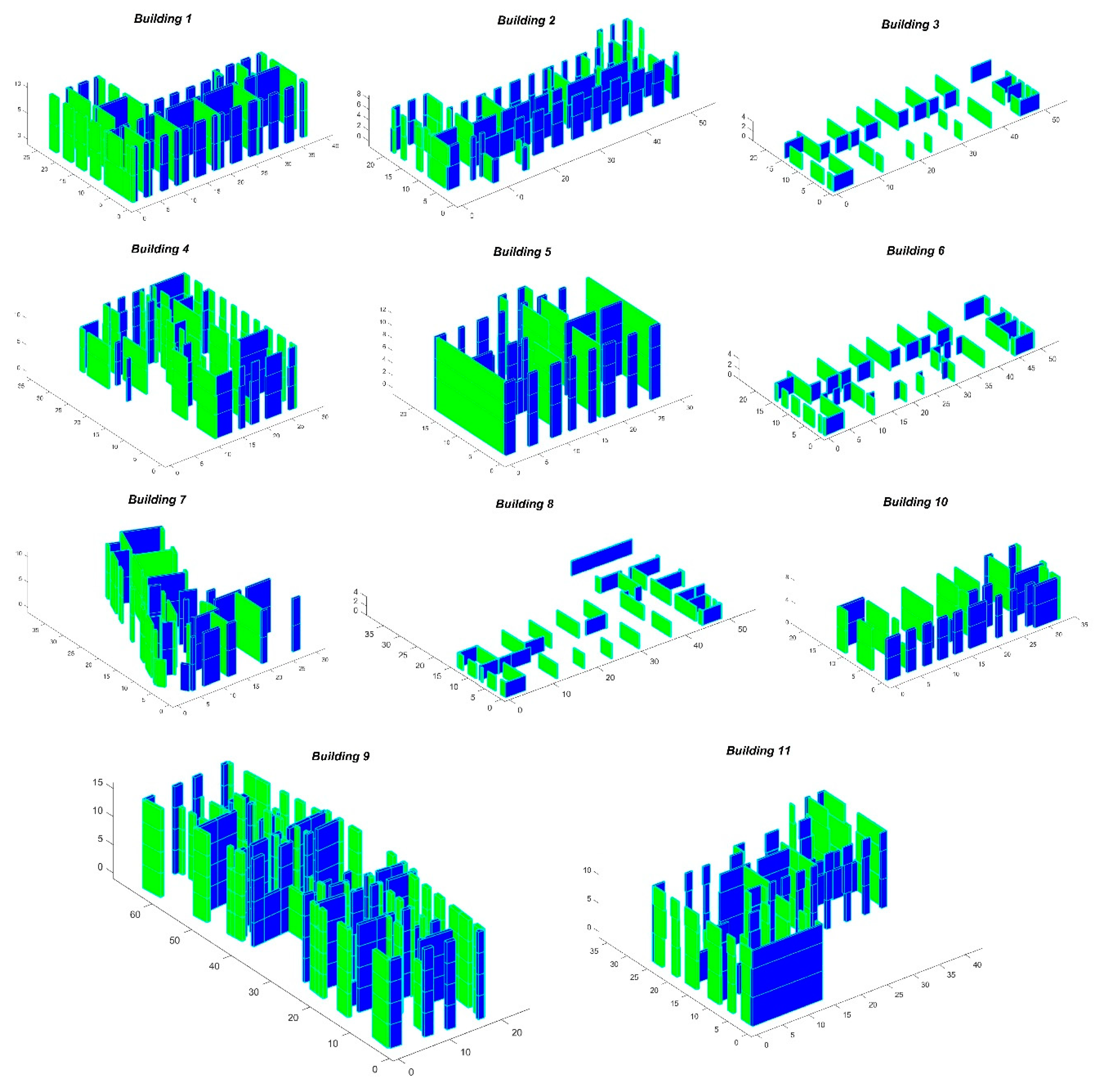
As mentioned before, a proper evaluation of the seismic performance requires a suitable definition of masonry mechanical parameters, duly considering that masonry is a non-homogeneous material characterized by an inelastic and anisotropic behavior. The identification of the appropriate force-displacement response of in-plane loaded walls is then particularly crucial as it significantly influences the results [4]. Moreover, depending on the material as well as on the texture, several masonry types can be detected in existing buildings, characterized by mechanical parameters varying in a very wide range. Anyhow, stiffness identification [24,25] and evaluation of drift capacity of in-plane loaded walls [26,27] are still critical issues [28].

Flat jacks, diagonal compression and shear compression tests, in situ or in laboratory conditions, are the subject of a wide literature concerning the shear resistance of masonry walls. But their outcomes are often contradictory; in fact, the values of mechanical parameters depend on the test procedure and may vary significantly for the same class of masonry or even for the same wall [24,25]. In this respect, guidelines for application of the Italian Building Code [29] provide some guidance, about the classification of masonry in terms of quality and typology.

The probabilistic seismic assessment procedure proposed here has been applied to 11 case studies suitably chosen among the masonry buildings under investigation. For the sake of the study, masonry has been mainly classified based on visual inspection and double flat-jack compressive test results, duly taking into account epistemic and aleatoric uncertainties affecting the force displacement response of in-plane loaded walls.

3. Case Studies

The aforementioned set of buildings, numbered from B1 to B11, are representative of a rather long historical period, since they were built between 1900 and 1980. The set includes: 3 single-story buildings (B3, B6 and B8), 4 two-story building (B1, B2, B7 and B10), 3 three-story buildings (B4, B5 and B11) and one four-story building (B10).

The buildings, mainly built with irregular stone and brick masonry characterized by different quality and workmanship skill, have been selected in order to cover wide ranges in terms of structural typologies, dimensions (volume varies between 3700 m³ and 45,000 m³) and inter-story heights (height varies between 3 m and 5 m).

The 3D arrangements of the seismic resistant walls of the investigated buildings is synthesized in Figure 8.

4. Methodology

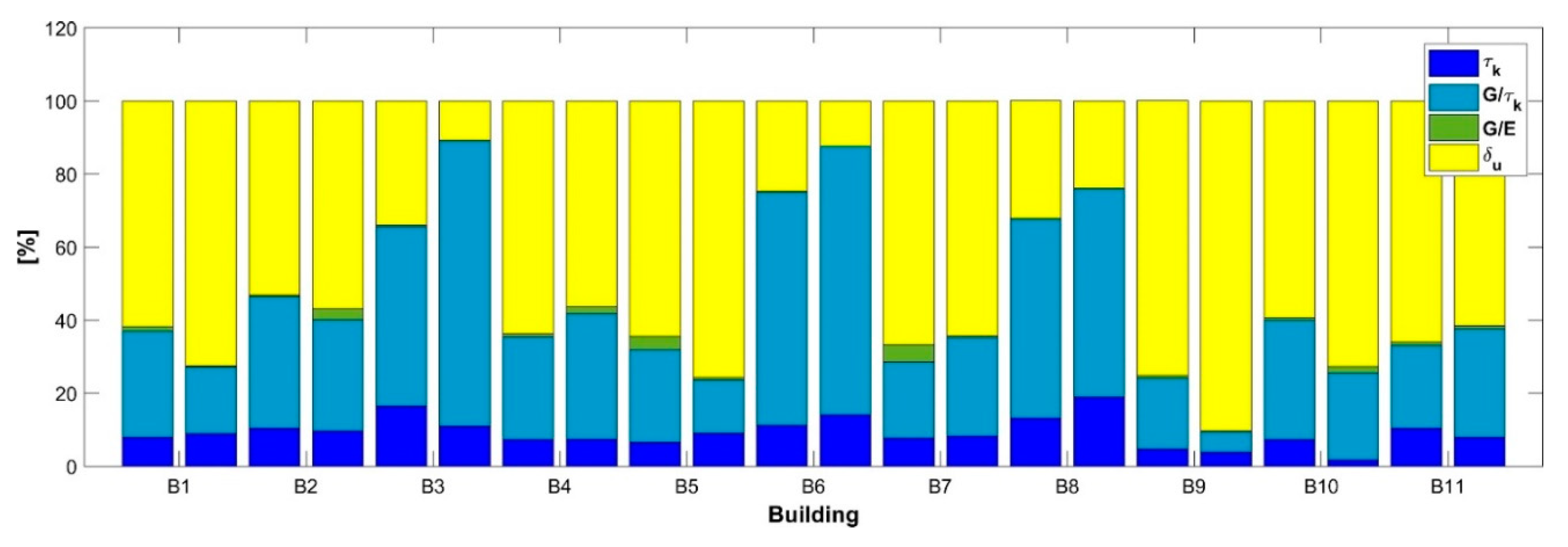
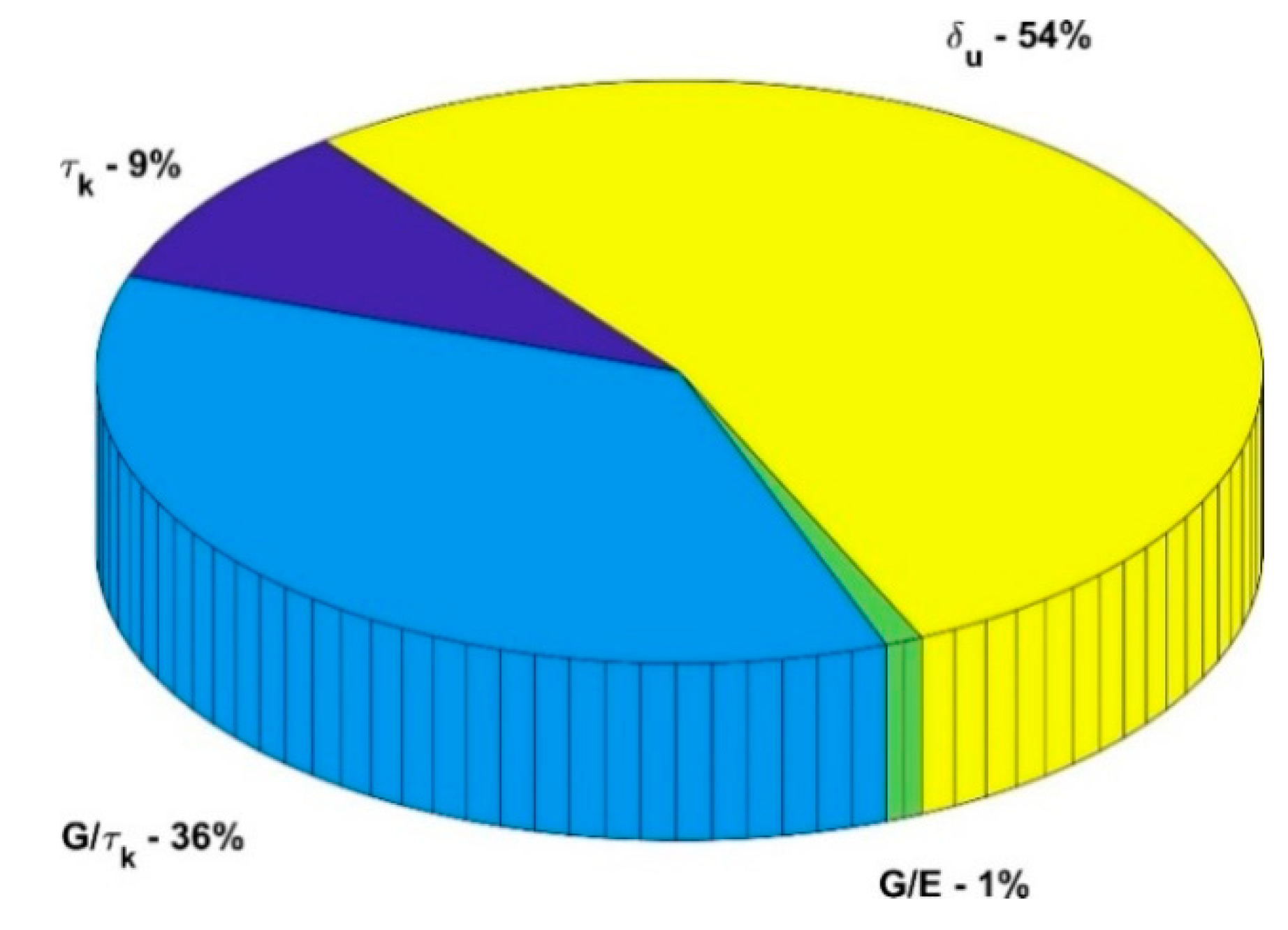
4.1. Identification of Uncertain Parameters

As discussed in the previous paragraph, the shear behavior of masonry walls is characterized by significant uncertainty regarding the stiffness identification, the displacement capacity and the ultimate strength.

In non-linear static analysis, the hysteretic behavior of masonry walls subjected to constant vertical load and cyclic horizontal loads is idealized by means of a bi-linear resistance envelope.

As anticipated, the bi-linear envelope is characterized by an initial elastic slope, defined by the lateral stiffness k and by a plastic plateau, bounded by the elastic inter-story drift ${\delta }_e$ and by the ultimate inter-story drift ${\delta }_u$, corresponding to the shear resistance of the wall $H_{Rd}$ (see Figure 9).

Assuming both ends are clamped, the lateral stiffness k of a masonry wall can be calculated, taking into account shear deformations and bending effects [30], as:

$$k=\frac{GA}{1.2h}{\left(1+\frac{G}{1.2E}{\left(\frac{h}{l}\right)}^2\right)}^{-1},$$

(13)

where h is the inter-story height of the wall, l its length, A the area of its cross-section, and E and G are the modulus of elasticity and the shear modulus of masonry respectively.

If diagonal tension shear failure governs, the shear resistance of the wall $H_{Rd}$ can be derived from

$$H_{Rd}=A\frac{1.5{\tau }_k}{b}\sqrt{1+\frac{{\mathsf{\sigma }}_0}{1.5{\tau }_k}},$$

(14)

where ${\sigma }_0$ is the compressive stress induced in the wall by the seismic load combination, ${\tau }_k$ is the shear strength of masonry and b is the shear resistance factor. The shear resistance factor depends on the aspect ratio of the wall, $h/l$. When $h/l\ge 1.5$, it can be assumed b = 1.5 [30].

Concerning the ultimate displacement, unreinforced masonry is characterized through the so called “ductility”. This property is far from being a ductility in a conventional sense [31], but rather a synthetic parameter accounting for the relative slip along crack surfaces that parts of the wall elements can sustain without significant shear stress loss. Wall ductility depends on normal stress ${\sigma }_0$ [31,32], on boundary conditions [13], as well as, via the aspect ratio $h/l$, of the wall geometry.

In the Eurocode 8—Part 3 [33] as well as in the guidelines for application of the Italian Building Code [29], the ultimate drift is defined as a percentage of the inter-story height of the wall, depending on the failure mode. For shear failure, the ultimate drift is set to

$${\delta }_u=0.4\%h.$$

(15)

Excluding geometric variables, uncertain parameters characterizing the definition of the force-displacement curve are:

• the shear modulus G and the elastic modulus E of masonry;
• the shear strength ${\tau }_k$;
• the ultimate displacement ${\delta }_u$.

For the purposes of the present study, suitable pdf has been derived for each relevant parameter, considering that the outcomes of seismic assessment are strongly dependent in non-trivial way, beside the adopted failure criterion, also on the probabilistic distributions of the material properties [34].

Following an approach similar to that proposed in [6], a normal distribution has been associated to the shear strength ${\tau }_k$. The mean value of ${\tau }_k$, ${\overline{\tau }}_k$, has been estimated combining in situ test results with the indications reported in [29], taking into account the masonry class and its qualitative features, while its standard deviation ${\sigma }_{\tau k}$ has been derived in such a way that 90% of the experimental data lies within the range of values given in [29] for the identified masonry class. In case of stone masonry, it has been obtained a coefficient of variation, $\mathrm{COV}={\sigma }_{\tau k}/{\overline{\tau }}_k=0.14$.

Regarding the shear modulus, due to belittle consideration influence of anisotropy and cracking of masonry, it seems that values provided in almost all national codes [29] as well as in Eurocode 6 [35] overestimate the actual values as reported in [24,36]. Based on a critical analysis of a large database of experimental test results [25], empirical relationships can be found for shear modulus and elastic modulus:

$$G={\alpha }_1 {\tau }_k,$$

(16)

$$G={\alpha }_{2}E,$$

(17)

where ${\alpha }_1=G/{\tau }_k$, is a normally distributed uncertain parameter with mean value 1500 and coefficient of variation 0.3, while ${\alpha }_2=G/E$, is again normally distributed with mean 0.15 and coefficient of variation 0.2.

For the ultimate displacement ${\delta }_u$, a database of test results is collected and analyzed in [26] and [27], mirroring the high variability of this parameter. A median value ${\delta }_u=0.47\%h$ is reported in [26] in case of shear failure, which is in accordance with the value of ${\delta }_u=0.4\%h$ given in Eurocode 8—Part 3 [33] and the Italian Building Code. Since in [26] a minimum value of $0.14\%h$ is given for ${\delta }_u$, ${\delta }_u$ can be assumed normally distributed with mean value equal to $0.4\%h$ and coefficient of variation 0.2, so that the minimum value $0.14\%h$ corresponds to the 0.1 fractile.

The statistical models adopted to model uncertain parameters are summarized in

Table 1. Statistical description of uncertain parameters.

Random Variable	$\overline{\mathit{X}}$	COV
${\tau }_k$	Mean Value for each masonry class in [29], e.g., 0.026 N/mm2 for stone	0.14
$G/{\tau }_k$	1500	0.3
$G/E$	0.15	0.2
${\delta }_u$	0.004	0.2

, in terms of mean values ($\overline{X})$ and the coefficient of variation (COV).

4.2. Sensitivity Analysis

Sensitivity analysis has been performed on the aforementioned set of case studies in order to quantify the relevance of each parameter in the evaluation of the seismic risk index.

Response surface methods based on general polynomial chaos expansions [37] have been used to represent uncertain parameters and their propagation through the models.

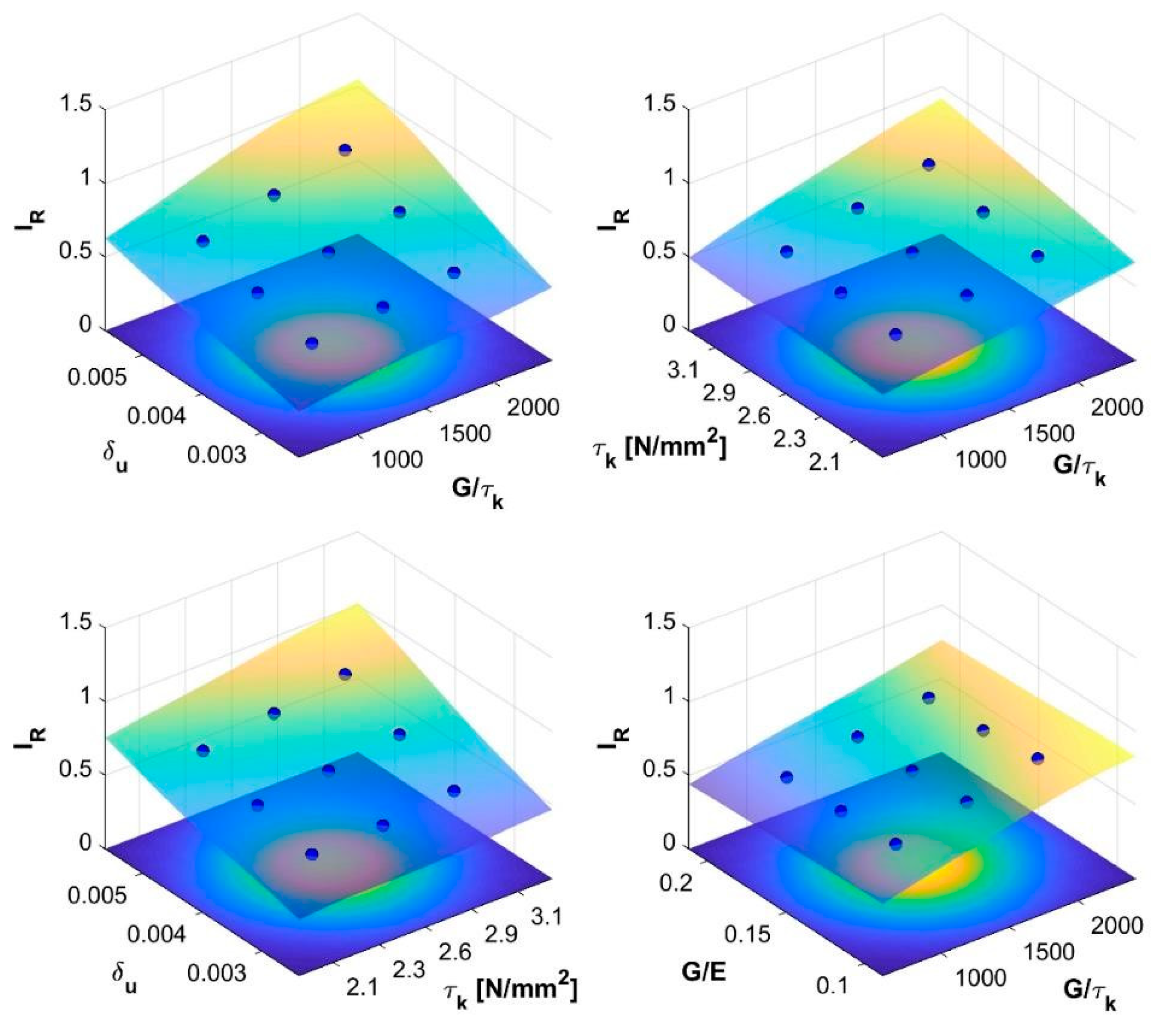
4.2.1. Response Surface via generalized Polynomial Chaos Expansion

Let $\mathit{Q}:\Omega \to {\mathbb{R}}^{nq}$ the vector of input random parameters [ ${\tau }_k$; $G/{\tau }_k$; $G/E$; ${\delta }_u$], described in the previous paragraph, characterizing the mechanical model, said $\Omega$ the set of possible events. The epistemic uncertainty coming from our lack of knowledge is modelled by this randomness, at which prior probability distributions $\pi \left(q\right)$ have been assigned in Table 1, based on professional expertise. For mathematical convenience we also introduce maps $F:\Omega \to {\mathbb{R}}^n$. These maps associate the set of random variables to a set of mutually independent random variables $Z_i$, $Z_i:\Omega \to {\mathbb{R}}^n$, characterized by standard normal distributions $\pi \left(z_i\right)$.

Then, the non-linear static analysis algorithm E-PUSH can be viewed as the forward model $\tilde{G}$, a deterministic solver that takes as input a given set of parameters q and provides a unique response vector $\mathit{u}$

$$\mathit{u}=\tilde{G}\left(\mathit{q}\right),$$

(18)

where u is a vector that gathers the response quantities, in this case the seismic risk index I_R.

Performing uncertainty quantification analysis consists in running the forward model $\tilde{G}$ many times to quantify the uncertainty of the output and may require an high computational cost. In order to speed up the computations, a proxy model for the predicted measurable u replacing the $\tilde{G}$ map can be of great use. Taking advantage of functional approximations of the random variables by means of the generalized polynomial chaos (gPC) expansion, the construction of response surfaces is significantly facilitated and a computationally cheap proxy model is obtained [38]. For an extensive review of this topic, please refer to [39].

Without going here into much mathematical detail, assuming that $\mathit{U}=\tilde{G}\left(\mathit{Q}\right)$ has a finite variance, the ${\mathit{U}}_N$ approximation of the response reads:

$$\mathit{U}=\tilde{G}\left(F^{-1}\left(\mathit{Z}\right)\right)\approx {\mathit{U}}_N={{\displaystyle \sum }}_{\left|\mathit{i}\right|\le N}{\widehat{\mathit{u}}}_i{\Phi }_{\mathit{i}}\left(\mathit{Z}\right).$$

(19)

In Equation (19) ${\Phi }_i\left(\mathit{Z}\right)={\varphi }_{i_1}\dots {\varphi }_{i_n}$ are the multivariate gPC basis functions, some orthogonal polynomials of total degree less than or equal to N, which is the degree at which the expansion is truncated; $\mathit{Z}$ is a Gaussian vector whose corresponding orthogonal polynomials are the Hermite polynomials, which are orthogonal with respect to the Gaussian measure; ${\widehat{\mathit{u}}}_{\mathit{i}}$ are the coefficients of the PCE, $\mathit{i}=\left(i_1,\dots ,i_n\right)\in {\mathit{N}}_0^n$ is a multiindex (with $\left|\mathit{i}\right|=i_1+\dots +i_n$).

The computation of the coefficients can be carried out with different methods such as the interpolation/regression, and the pseudo-spectral projection. Further details about this topic are given in [39,40]. When the gPC expansion of a given forward model is available, one has in fact an analytical representation of u in terms of z, with the advantage that for any realization of the random vector $\mathit{Q}$ the response u can be easily evaluated by first mapping q to z and then evaluating the gPC expansion without much computational expense.

The response surface is then obtained by running few times the forward model in correspondence of the integration points determined via Gaussian quadrature rule for the random parameters. In this specific case, a degree six polynomial expansion has been used (2401 integration points) and the accuracy of the response given by the surrogate model has been assessed checking that it fits the exact solution.

As an example, the response surfaces obtained for seismic risk index of the first case study (Building 1) are reported in the four diagrams in Figure 10:

• in terms of $G/{\tau }_k$ and ${\delta }_u$, assuming mean values for ${\tau }_k$ and $G/E$;
• in terms of $G/{\tau }_k$ and ${\tau }_k$, assuming mean values for ${\delta }_u$ and $G/E$;
• in terms of ${\tau }_k$ and ${\delta }_u$, assuming mean values for $G/{\tau }_k$ and $G/E$;
• in terms of $G/{\tau }_k$ and $G/E$ assuming mean values for ${\tau }_k$ and ${\delta }_u$.

4.2.2. Evaluation of Sobol Indices

As demonstrated in [41], it must be remarked that, besides providing a complete representation of the random response of a model, the gPC expansion also allows an analytical derivation of Sobol indices [42,43], so avoiding Monte Carlo simulations, which are much more computationally demanding.

Sobol indices, which measure the quota of the total variance referable to the uncertainties of each input parameters, are recognized to be accurate descriptors of the sensitivity of the model since they do not assume any kind of linearity or monotonicity of the model [43].

Once the gPC representation of the model is available, the Sobol indices $S_q$ can be analytically computed as

$$S_q={{\displaystyle \sum }}_{\left|\mathit{i}\right|\le N}\frac{{{\widehat{\mathit{u}}}_i}^{2}E[{\Phi }_i{\left(Z\right)}^2]}{D_{PC}},$$

(20)

where $D_{PC}$ is total variance of the response.

Referring to the 11 case studies, the results of the sensitivity analysis, carried out considering both relevant direction of application of the seismic action, are summarized in Figure 11. These results demonstrate that the most relevant model parameters influencing the total variance are ultimate displacement ${\delta }_u$ (≈54% of the total variance) and the $G/{\tau }_k$ ratio (≈36% of the total variance) and, to a lesser extent, the shear strength ${\tau }_k$ (≈9% of the total variance), while the influence of $G/E$ ratio is negligible, as it represents only the 1% of the total variance (see Figure 12).

It must be underlined that in the considered case the sum of contributions to the total variance associated with ${\tau }_k$ and $G/{\tau }_k$ is not particularly sensitive on the scattering of ${\tau }_k$. For example, when the coefficient of variation of the shear strength increases from 0.14 to 0.2, the contribution of ${\tau }_k$ raises to 19% of the total variance, while the contribution of $G/{\tau }_k$ decreases to 30%., but the total variance associated to both contributions remain almost the same (≈49% vs. ≈45%).

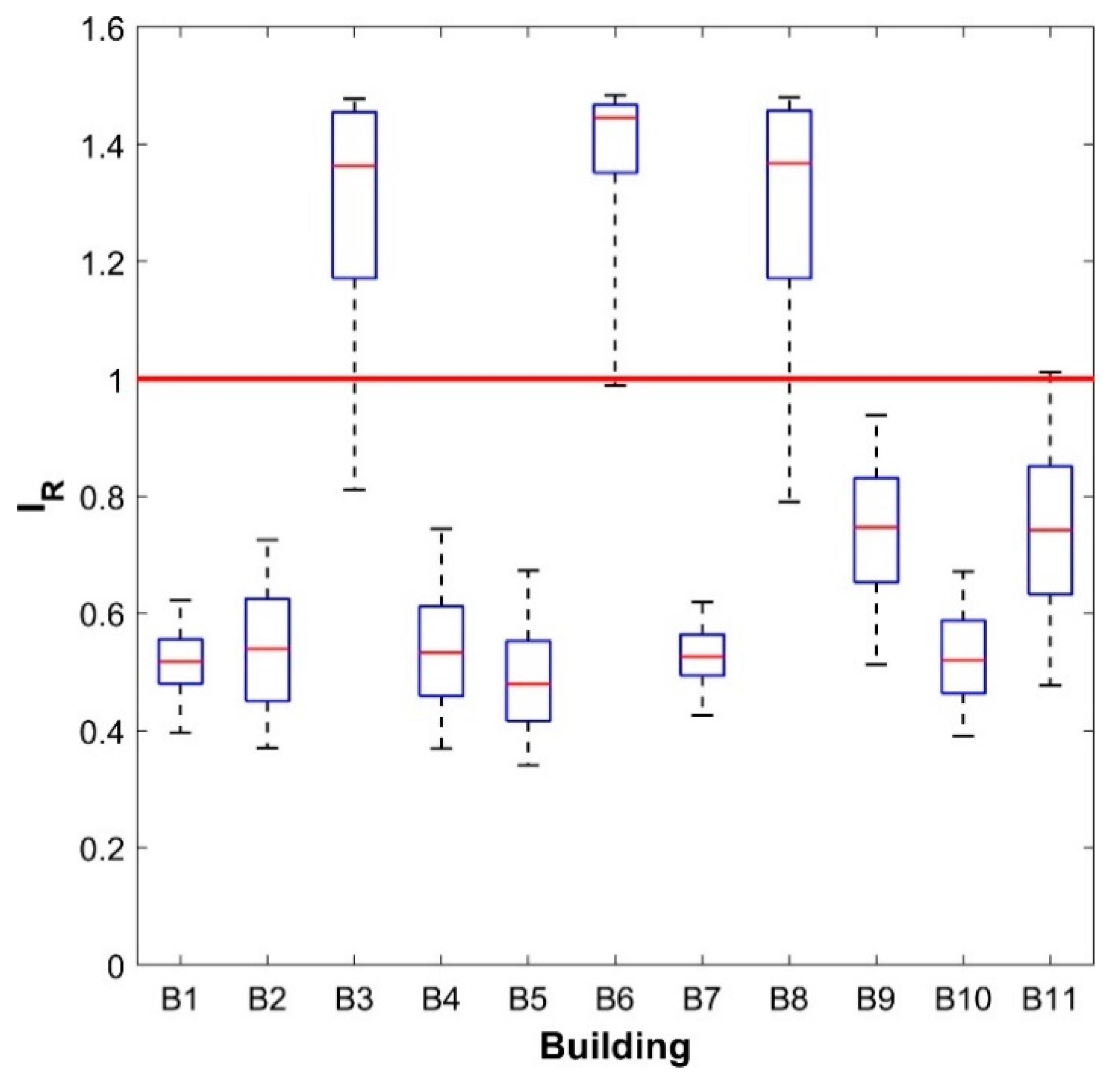
4.3. Uncertainty Quantification

From the response surfaces previously defined, statistics of the seismic risk index can be finally easily computed quantifying the uncertainty in the results and providing an important information for the performance classification of the investigated structures.

In

Table 2. Statistics of seismic risk index in the 11 case studies.

School Building	${\mathit{I}}_{\mathit{R},05}$	${\mathit{I}}_{\mathit{R},50}$	${\mathit{I}}_{\mathit{R},95}$
B1	0.40	0.52	0.62
B2	0.37	0.54	0.73
B3	0.81	1.37	1.48
B4	0.37	0.53	0.74
B5	0.34	0.48	0.67
B6	0.99	1.45	1.48
B7	0.43	0.53	0.62
B8	0.79	1.37	1.48
B9	0.51	0.75	0.94
B10	0.39	0.52	0.67
B11	0.48	0.74	1.01

and in the box-plot in Figure 13, the results in terms of median values, 5-th and 95-th percentiles are reported for the 11 case studies considering the most relevant direction of application of the seismic action.

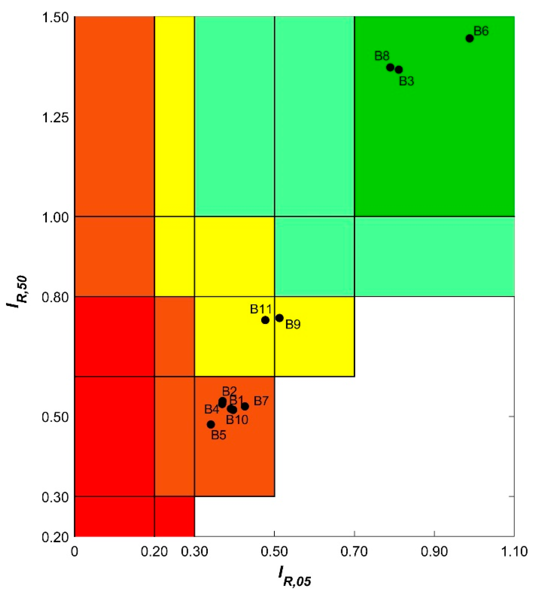
5. Seismic Performance Classification

As already underlined, a robust and reliable performance classification of buildings is of paramount importance in decision-making strategies about seismic retrofit.

In order to introduce a suitable performance indicator, a performance classification, based on the probabilistic risk assessment performed in the previous section, is proposed here.

Seismic risk categories are identified considering the median value (I_R,50) and the 5th percentile (I_R,05) of the seismic risk index. In particular, five categories (A–E) with increasing magnitude of vulnerability are defined according the interval reported in

Table 3. Seismic performance classification—definition of categories.

		${\mathit{I}}_{\mathit{R},05}$
		<0.2	0.2–0.3	0.3–0.5	0.5–0.7	>0.7
$I_{R,50}$	<0.3	E	E	-	-	-
	0.3–0.6	E	D	D	-	-
	0.6–0.8	E	D	C	C	-
	0.8–1	D	C	C	B	B
	>1	D	C	B	B	A

.

Allowing us to quantify and to communicate risks, the seismic performance classification defined in Table 3 could represent an important tool for stakeholders to undertake decision about seismic retrofit strategies, helping them to prioritize the interventions for the most vulnerable structures.

Focusing the attention on the buildings investigated, the classification proposed in Table 3 leads to the classification: single-story buildings B3, B6 and B8 are in class A, buildings B9 and B11 are in class C, and buildings B1, B2, B4, B5, B7 and B10 result in being in class D (see Figure 14).

6. Conclusions

In this paper, a methodology for the probabilistic assessment of the seismic risk index of existing masonry buildings is proposed.

Starting from a simplified non-linear pushover-type algorithm developed by the authors, the procedure allows us to quantify the propagation of uncertainties related to masonry parameters in the resulting seismic risk index.

The procedure is based on the definition of response surfaces for the seismic risk indices I_R through gPC-expansion; in this way, quantification of uncertainties in the resulting seismic risk index is easily obtained, reducing the computation effort, and Sobol sensitivity indices can be computed analytically from the gPCE coefficients.

The main sources of uncertainties, related to masonry material parameters and in-plane displacement capacity, have been investigated and, by means of sensitivity analysis, their impact in the evaluation of seismic risk indices has been quantified. The results confirm that the most relevant parameters are related to definition of the ultimate displacement ${\delta }_u$ and the shear modulus G, highlighting the necessity for further investigations on the shear behavior of masonry walls.

Finally, a seismic performance classification has been presented, defining five seismic risk categories on the basis of the median value (I_R,50) and the 5th percentile (I_R,05) of the seismic risk index.

The outcomes have been illustrated for a set of existing masonry buildings that are part of the school system in the Municipality of Florence, demonstrating how the presented procedure is very promising and provides a robust and reliable tool to support decisions about seismic retrofit and the priority of interventions for existing masonry buildings.

References

1. Croce, P.; Beconcini, M.L.; Formichi, P.; Cioni, P.; Landi, F.; Mochi, C.; Castelluccio, R. Expeditious assessment of seismic vulnerability of existing buildings from a statistic sample of school buildings, property of the Comune di Firenze (in Italian). Proceedings of XVII convegno ANIDIS “L’ingegneria sismica in Italia”, Pistoia, Italy, 17–21 September 2017; Pisa University Press: Pisa, Italy. [Google Scholar]
2. Roca, P.; Cervera, M.; Gariup, G.; Luca, P. Structural analysis of masonry historical constructions. Classical and advanced approaches. Arch. Comput. Methods Eng. 2010, 17, 299–325. [Google Scholar] [CrossRef]
3. Lourenço, P.B. Computations on historic masonry structures. Prog. Struct. Eng. Mater. 2002, 4, 301–319. [Google Scholar] [CrossRef]
4. Croce, P.; Beconcini, M.L.; Formichi, P.; Cioni, P.; Landi, F.; Mochi, C.; Giuri, R. Influence of mechanical parameters on non linear static analysis of masonry walls: A relevant case study. Procedia Struct. Integr. 2018, 11, 331–338. [Google Scholar] [CrossRef]
5. Borri, A.; Corradi, M.; Castori, G.; De Maria, A. A method for the analysis and classification of historic masonry. Bull. Earthq. Eng. 2015, 13, 2647–2665. [Google Scholar] [CrossRef]
6. Bracchi, S.; Rota, M.; Magenes, G.; Penna, A. Seismic assessment of masonry buildings accounting for limited knowledge on materials by Bayesian updating. Bull. Earthq. Eng. 2016, 14, 2273–2297. [Google Scholar] [CrossRef]
7. Beconcini, M.L.; Cioni, P.; Croce, P.; Formichi, P.; Landi, F.; Mochi, C. Non-linear static analysis of masonry buildings under seismic actions. In Proceedings of the 12th International Multi-Conference on Society, Cybernetics and Informatics: IMSCI 2018, Orlando, FL, USA, 8–11 July 2018. [Google Scholar]
8. Croce, P.; Holicky, M. Operational Methods for the Assessment and Management of Aging Infrastructure; TEP: Pisa, Italy, 2015. [Google Scholar]
9. Tomazevic, M.; Turnsek, V.; Tertelj, S. Computation of the Shear Resistance of Masonry Buildings; Report ZRMK-ZK; Institute for Testing and Research in Materials and Structures: Ljubljana, Slovenia, 1978. (In Slovene) [Google Scholar]
10. Tomazevic, M. Improvement of Computer Program POR; Report ZRMK-IK; Institute for Testing and Research in Materials and Structures: Ljubljana, Slovenia, 1978. (In Slovene) [Google Scholar]
11. Regione Autonoma Friuli Venezia Giulia. TD n.2—Guidelines for Strengthening and Repair of Masonry Buildings; Gruppo Interdisciplinare Centrale: Udine, Italy, 1980. (In Italian) [Google Scholar]
12. Ministry of Public Works. Guidelines for Application of Structural Code for Strengthening and Repair of Masonry Buildings; Istituto Poligrafico e Zecca dello Stato: Roma, Italy, 1981. (In Italian) [Google Scholar]
13. Magenes, G. A method for pushover analysis in seismic assessment of masonry buildings. In Proceedings of the 12th World Conference on Earthquake Engineering, Auckland, New Zealand, 30 January–4 February 2000. [Google Scholar]
14. Fajfar, P.; Eeri, M. A Nonlinear Analysis Method for Performance Based Seismic Design. Earthq. Spectra 2000, 16, 573–592. [Google Scholar] [CrossRef]
15. Italian Ministry of Infrastructure and Transport. NTC 2018—Italian Building Code; D.M. 17 January 2018; Istituto Poligrafico e Zecca dello Stato: Roma, Italy, 2018. (In Italian) [Google Scholar]
16. Vidic, T.; Fajfar, P.; Fischinger, M. Consistent inelastic design spectra: Strength and displacement. Earthq. Eng. Struct. Dyn. 1994, 23, 502–521. [Google Scholar] [CrossRef]
17. Miranda, E.; Bertero, V.V. Evaluation of Strength Reduction Factors for Earthquake-Resistant Design. Earthq. Spectra 1994, 10, 357–379. [Google Scholar] [CrossRef]
18. Miranda, E. Inelastic displacement ratios for displacement based earthquake resistant design. In Proceedings of the 12th World Conference on Earthquake Engineering, Auckland, New Zealand, 30 January–4 February 2000. [Google Scholar]
19. EN1998-1. Eurocode 8: Design of Structures for Earthquake Resistance—Part 1: General Rules, Seismic Actions and Rules for Buildings; CEN: Brussels, Belgium, 2004. [Google Scholar]
20. Bothara, J.K.; Dhakal, R.P.; Mander, J.B. Seismic performance of an unreinforced masonry building: An experimental investigation. Earthq. Eng. Struct. Dyn. 2010, 39, 45–68. [Google Scholar] [CrossRef]
21. Ahmad, N.; Crowley, H.; Pinho, R.; Ali, Q. Simplified formulae for the displacement capacity, energy dissipation, and characteristic vibration period of brick masonry buildings. In Proceedings of the 8IMC-International Masonry Conference, Dresden, Germany, 4–7 July 2010; pp. 1385–1394. [Google Scholar]
22. Yi, T.; Moon, F.L.; Leon, R.T.; Kahn, L.F. Lateral Load Tests on a Two-Story Unreinforced Masonry Building. J. Struct. Eng. 2006, 132, 643–652. [Google Scholar] [CrossRef]
23. Aedes Software. Aedes PCM User’s Manual; Aedese Software per Ingegneria Civile: San Miniato, Italy, 2016. (In Italian) [Google Scholar]
24. Bosiljkov, V.Z.; Totoev, Y.Z.; Nichols, J.M. Shear modulus and stiffness of brickwork masonry: An experimental perspective. Struct. Eng. Mech. 2005, 20, 21–43. [Google Scholar] [CrossRef]
25. Croce, P.; Beconcini, M.L.; Formichi, P.; Cioni, P.; Landi, F.; Mochi, C.; De Lellis, F.; Mariotti, E.; Serra, I. Shear modulus of masonry walls: A critical review. Procedia Struct. Integr. 2018, 11, 339–346. [Google Scholar] [CrossRef]
26. Petry, S.; Beyer, K. Influence of boundary conditions and size effect on the drift capacity of URM walls. Eng. Struct. 2014, 65, 76–88. [Google Scholar] [CrossRef]
27. Wilding, B.V.; Beyer, K. Analytical and empirical models for predicting the drift capacity of modern unreinforced masonry walls. Earthq. Eng. Struct. Dyn. 2018, 47, 2012–2031. [Google Scholar] [CrossRef]
28. Beconcini, M.L.; Cioni, P.; Croce, P.; Formichi, P.; Landi, F.; Mochi, C. Influence of shear modulus and drift capacity on non-linear static analysis of masonry buildings. In IABSE Symposium, Guimaraes 2019: Towards a Resilient Built Environment Risk and Asset Management, Report; International Association for Bridge and Structural Engineering (IABSE): Zurich, Switzerland, 2019; pp. 876–883. ISBN 978-385748163-5. [Google Scholar]
29. Italian Public Works Council. Guidelines for Application of Italian Building Code; Istituto Poligrafico e Zecca dello Stato: Roma, Italy, 2019. (In Italian) [Google Scholar]
30. Tomazevic, M. Shear resistance of masonry walls and Eurocode 6: Shear versus tensile strength of masonry. Mater. Struct. 2009, 42, 889–907. [Google Scholar] [CrossRef]
31. Lang, K. Seismic Vulnerability of Existing Buildings. Ph.D. Thesis, ETH Zurich, Zurich, Switzerland, 2002. [Google Scholar]
32. Ganz, H.R.; Thürlimann, B. Versuche an Mauerwerksscheiben unter Normalkraft und Querkraft; Inst. für Baustatik und Konstruktion, ETH Zürich, Report Nr. 7502-4; Birkhäuser Verlag: Basel, Switzerland, 1984. [Google Scholar]
33. EN1998-3. Eurocode 8: Design of Structures for Earthquake Resistance—Part 3: Assessment and Retrofitting of Buildings; CEN: Brussels, Belgium, 2005. [Google Scholar]
34. Croce, P.; Beconcini, M.L.; Formichi, P.; Landi, F.; Puccini, B.; Zotti, V. Seismic risk evaluation of existing masonry buildings: Methods and uncertainties. In IABSE Congress New York: The Evolving Metropolis; IABSE: Zurich, Switzerland, 2019; pp. 2510–2515. ISBN 978-385748165-9. [Google Scholar]
35. EN1996-1-1. Eurocode 6: Design of Masonry Structures—Part 1-1: Common Rules for Reinforced and Unreinforced Masonry Structures; CEN: Brussels, Belgium, 2005. [Google Scholar]
36. Zimmermann, T.; Strauss, A.; Wendner, R. Old Masonry under Seismic Loads: Stiffness Identification and Degradation. In Proceedings of the Structures Congress 2011 ASCE, Las Vegas, NV, USA, 14–16 April 2011; pp. 1736–1747. [Google Scholar] [CrossRef]
37. Ghanem, R.G.; Spanos, P.D. Stochastic Finite Elements—A Spectral Approach; Springer: Berlin, Germany, 1991. [Google Scholar]
38. Landi, F.; Marsili, F.; Friedman, N.; Croce, P. A comparison of stochastic inverse methods with sampling and functional-based linear and non-linear update procedures Beton. und Stahlbetonbau Spezial 2018. In Proceedings of the 16th International Probabilistic Workshop, Extended Abstract, Vienna, Austria, 12–14 September 2018. [Google Scholar] [CrossRef]
39. Xiu, D. Numerical Methods for Stochastic Computations; Princeton University Press: Princeton, NJ, USA, 2010. [Google Scholar]
40. Matthies, H.G.; Zander, E.K.; Rosic, B.V.; Litvinenko, A.; Pajonk, O. Inverse Problems in a Bayesian Setting. In Computational Methods for Solids and Fluids; Ibrahimbegovic, A., Ed.; Springer: Cham, Switzerland, 2016; Volume 41, pp. 245–286. [Google Scholar] [CrossRef]
41. Sudret, B. Global sensitivity analysis using polynomial chaos expansions. Reliab. Eng. Syst. Saf. 2008, 93, 964–979. [Google Scholar] [CrossRef]
42. Sobol, I. Sensitivity estimates for nonlinear mathematical models. Math. Model. Comput. Exp. 1993, 1, 407–414. [Google Scholar]
43. Saltelli, A.; Sobol, I. About the use of rank transformation in sensitivity of model output. Reliab. Eng. Syst. Saf. 1995, 50, 225–239. [Google Scholar] [CrossRef]
Figure 1. Final output of the pushover analysis, verification in the acceleration-displacement response spectra (ADRS) plane.
Buildings 09 00237 g001
Figure 2. Verification in the ADRS plane parameterized as a function of the damping coefficient ξ .
Buildings 09 00237 g002
Figure 3. Variation of seismic risk index as a function of damping coefficient ξ .
Buildings 09 00237 g003
Figure 4. Sketch of the two story masonry structure tested at Georgia Tech laboratory [22], plan view and elevation.
Buildings 09 00237 g004
Figure 5. 3D layout of shear walls in E-PUSH.
Buildings 09 00237 g005
Figure 6. Comparison of capacity curves of walls A and B with experimental H δ test results [22].
Buildings 09 00237 g006
Figure 7. Comparison of capacity curves of walls 1 and 2 with experimental H δ test results [22].
Buildings 09 00237 g007
Figure 8. Three-dimensional (3D) layout of the resistant shear walls for the investigated masonry buildings.
Buildings 09 00237 g008
Figure 9. Bi-linear envelope, shear behavior masonry walls.
Buildings 09 00237 g009
Figure 10. Response surfaces for the seismic risk index IR (Building 1).
Buildings 09 00237 g010
Figure 11. Sobol indices for τk, Gk, G/E and δu in the investigated buildings.
Buildings 09 00237 g011
Figure 12. Mean values of Sobol sensitivities in the investigated buildings.
Buildings 09 00237 g012
Figure 13. Box plot of seismic risk indexes for the 11 masonry buildings considered in the study.
Buildings 09 00237 g013
Figure 14. Seismic performance classification of the investigated buildings.
Buildings 09 00237 g014