Representing Small Commercial Building Faults in EnergyPlus, Part I: Model Development

Abstract

Small commercial buildings (those with less than approximately 1000 m² of total floor area) often do not have access to cost-effective automated fault detection and diagnosis (AFDD) tools for maintaining efficient building operations. AFDD tools based on machine-learning algorithms hold promise for lowering cost barriers for AFDD in small commercial buildings; however, such algorithms require access to high-quality training data that is often difficult to obtain. To fill the gap in this research area, this study covers the development (Part I) and validation (Part II) of fault models that can be used with the building energy modeling software EnergyPlus^® and OpenStudio^® to generate a cost-effective training data set for developing AFDD algorithms. Part I (this paper) presents a library of fault models, including detailed descriptions of each fault model structure and their implementation with EnergyPlus. This paper also discusses a case study of training data set generation, representing an actual building.

1. Introduction

Building faults, meaning improper or undesirable operations of building systems and equipment, are common in modern commercial buildings. In the United States, recent studies estimate that faults increase commercial primary energy consumption by 90–530 TWh (0.3–1.8 quadrillion Btu [quads]) [1]. Given that the detection and correction of faults represents a large energy savings opportunity, significant effort has been dedicated to the research, development, and deployment of fault detection and diagnosis (FDD) algorithms [2,3,4].

The availability of accurate physical models for building faults advances several key areas of FDD research, including the projection of regional or national fault energy impacts [1,5,6], development of model-based FDD algorithms [4,7,8], and simulation-based assessment of FDD algorithm performance [9,10]. For large-scale fault impact estimation, the availability of reliable fault impact data is a key challenge. Both Roth et al. [1] and Kim, Cai, and Braun [5] identify multiple gaps, uncertainties, and inconsistencies in the available literature regarding the average loss of efficiency resulting from various types of faults. Simulation studies, such as those performed by Fernandez et al. [11] and Li and O’Neill [6], offer a rigorous and consistent approach to estimating fault impacts, provided that the fault models used are well validated.

Similarly, data-driven FDD algorithms require large volumes of diverse training data, but large data sets of faulty behavior are expensive to obtain experimentally and impractical to glean from field data. However, simulated faults can be used indirectly to train data-driven FDD algorithms [7]. Simulation also offers key theoretical advantages over experimental or field data in the evaluation of FDD algorithms: the ground truth is known with greater certainty; the cost of generating evaluation samples is low; evaluation samples can be generated for a wide variety of equipment, building types, environmental conditions, and so on; and evaluation data sets may be constructed without significant gaps or biases [10,12]. However, an accurate simulation of faults is not trivial and rigorous validation is critical if the models are to be trusted [4,10].

In this two-part article series, we present the development and validation of a library of models for faults common in small commercial buildings in the United States. In Part I (Model Development—this paper), we describe the modeling approach and technical development; in Part II (Model Validation), we describe an experimental validation methodology for the developed models and the validation results. The remainder of this article is organized as follows: Section 2 surveys prior research in modeling building faults, Section 3 presents the methodology, and Section 4 describes the specific fault models developed, Section 5 provides a case study of fault model applications for generating a training data set, and Section 6 provides the conclusions of Part I.

2. Prior Work

This section reviews previous studies related to fault model development and provides an assessment of their limits and gaps. Although this study focuses on fault models that can be embedded in building energy simulation tools, it is relevant to review fault modeling methodologies that were covered in previous studies. These previous modeling methodologies are classified into three different types of approaches used to estimate degraded performance associated with faults: physical, semiempirical, and empirical.

Physical models can be further broken down into detailed and simplified approaches. Detailed physical modeling approaches have been applied primarily to heating, ventilation, and air-conditioning (HVAC) equipment. Studies that use detailed approaches typically involve the development of a system (e.g., vapor compression system, chiller, or air handling unit) model that couples multiple detailed component models in a manner that is based on the real system configuration [13,14,15,16,17,18,19,20,21,22,23,24,25]. For example, Cheung and Braun [13,14] developed physics-based models for components, such as compressors, condensers, expansion valves, evaporators, and refrigerant pipelines, where the parameters of the models were trained using measurement data for a range of different systems tested in the laboratory for both normal and fault operation. The faults were simulated by varying specific parameters in the component models or at the system level; these faults included compressor valve leakage, refrigerant liquid–line restriction, the presence of noncondensable gas in refrigerants, under/overcharge of refrigerants, and condenser/evaporator fouling. The advantage of these detailed models is that they can provide many specific states and other outputs that are affected by faults; however, they are not typically suitable for whole-building energy simulation because of their high computational requirements.

Simplified physical modeling approaches [11,26] often take advantage of physical parameters that are already defined in a building energy simulation tool. Faults such as a stuck economizer damper and biased sensors in the economizer fall into this category. Because component models related to certain fault types are often included in the building model, the effect of each of these faults can be estimated during the state computation of the building simulation at each time step. For instance, faults such as sensor bias can be simulated with the necessary level of detail using this simplified approach.

Some building simulation parameters that can be directly adjusted to simulate faults have a complex dependency on fault levels that may be difficult to represent using physical models. The work of Fernandez et al. [11] simulated the effect of the refrigerant undercharge fault by reducing the rated coefficient of performance (COP) and total cooling capacity defined in the cooling coil model at the beginning of the simulation, but this simplification neglects the variation in performance degradation under different operating conditions (e.g., outdoor air temperature and evaporator inlet temperature) throughout the simulation period. For instance, refrigerant undercharge in a vapor compression system can be simulated by modifying existing parameters in the building simulation, such as COP and capacity, which have a nonlinear dependence on charge. In these cases, empirical or semiempirical models [27,28,29,30,31] derived from measurements or detailed physical models can be used.

The empirical approach considered in previous studies is suitable for including greater fidelity in otherwise simplified fault models without substantially increasing computation time. Faults with less physical complexity are compatible with the simplified approach, whereas faults that require additional detail or fidelity for the fault impact estimation can be addressed with the empirical approach. For instance, empirical models that estimate the degraded COP and total cooling capacity of the roof top unit (RTU) at each time step based on varying operating conditions can be embedded in the building simulation tool to properly estimate changes in the degradation level. However, a proper formulation of the empirical model is essential for capturing fault characteristics and conforming to the requirements of the building simulation tool. Additionally, a representative training data set that includes the behavior of the fault is also necessary for training the empirical model.

Besides the use of fault modeling to predict the impact of different faults on building simulation outputs, other studies [1,5] estimate the nationwide impact of various faults in buildings. To do this, Roth et al. [1] carried out a comprehensive literature review to identify faults that occur in commercial buildings in the United States. The authors identified more than 100 faults and analyzed their nationwide annual energy impact, and the energy savings potential of control and diagnostic approaches, barriers to controls and diagnostics, and drivers for controls and diagnostics. This report includes detailed descriptions of different types of faults and provides a simplified method of estimating the energy impact of those faults. The characteristic information of various faults and the fault impact estimation approach from this study were adopted in Kim, Cai, and Braun [5], with the latest public information [32] to estimate the nationwide annual energy and financial impacts of faults that are common in small commercial buildings. Kim, Cai, and Braun [5] focused on the impact on commercial buildings that have a total floor area of less than 1000 m²; the prioritized fault list from this prior work was the basis to determine the various types of faults to be modeled in this study.

3. Methodology

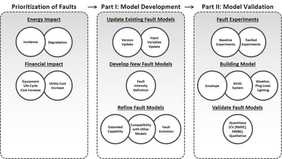
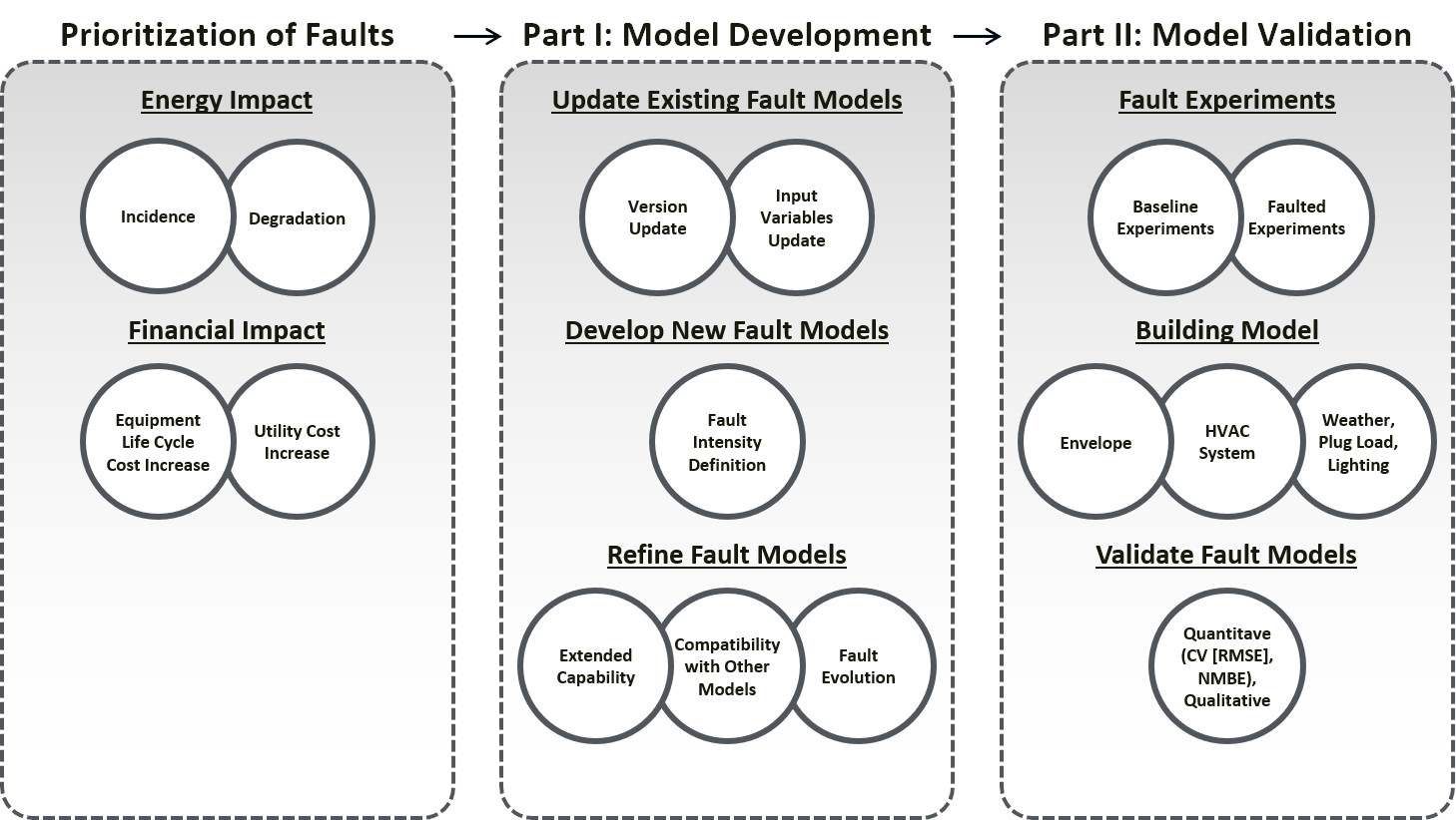
Figure 1 shows the workflow of the study documented in this paper and the companion (Part II) paper. The fault models considered in this study were those identified as highest priority by Kim, Cai, and Braun [5]. Based on an extensive literature review and communications with experts in the field, we estimated annual energy impact, reflecting the occurrence percentage and performance degradation of each fault, and the financial impact, reflecting the utility cost increase and life cycle cost increase of each fault. The estimates were used to prioritize faults that have a significant impact on nationwide energy consumption.

Models for all faults were implemented for the whole-building energy modeling software engine EnergyPlus^® [33], developed and maintained by the U.S. Department of Energy. Some of the fault models used were developed in a previous study [28]; those faults applicable to small commercial buildings were adopted and updated for this work by revising model inputs and version compatibility with EnergyPlus 9.1 and OpenStudio 2.8. The remaining faults in the list represent newly developed models with new fault intensity definitions. All fault models were refined to have extended capabilities, such as operation with a wider variety of modeling objects in EnergyPlus, compatibility with other fault models within the simulation, and additional features such as the fault evolution (see Section 4). A library of all fault models developed in this study is available in a public repository for future use cases [34].

Some, but not all, of the fault models were validated against experimental measurements. Simulation results with and without modeled faults were compared to actual experimental measurements obtained from a test facility designed to resemble a small office building. Validation results are described in Part II (Model Validation).

4. Fault Models

This section includes classification of all fault models based on modeling approaches and the differences between each approach, as well as descriptions of each fault model.

Table 1. List of Fault Models Considered in this Study.

Modeling Approach	Fault Measure Name	Fault Intensity Definition	Fault Intensity Range	Fault Evolution
Physical	Excessive infiltration around the building envelope	Ratio of excessive infiltration around the building envelope compared to the unfaulted condition	0 to 0.4	Y
	HVAC setback error: delayed onset	Delay in the onset of setback in hours	0 to 3 h	N
	HVAC setback error: early termination	Early termination of setback in hours	0 to 3 h	N
	HVAC setback error: no overnight setback	Absence of overnight setback (binary)	0 or 1	N
	Lighting setback error: delayed onset *	Delay in the onset of setback in hours	0 to 3 h	N
	Lighting setback error: early termination *	Early termination of setback in hours	0 to 3 h	N
	Lighting setback error: no overnight setback *	Absence of overnight setback (binary)	0 or 1	N
	Improper time delay setting in occupancy sensors *	Delayed time setting in hours	0 to 0.75 h	N
	Oversized equipment at design *	Ratio of increased sizing compared to the correct sizing	0 to 0.5	N
	Supply air duct leakages	Ratio of the leakage flow relative to supply flow	0 to 0.3	N
	Return air duct leakages *	Unconditioned air introduced to return air stream at full load condition as a ratio of the total return airflow rate	0 to 0.3	Y
	Thermostat measurement bias	Thermostat measurement bias in K	$-$3 to 3 K	Y
	Economizer opening stuck at certain position	Ratio of economizer damper at the stuck position (0 = completely closed, 1 = completely open)	0 to 1	N
	Biased economizer sensor: mixed temperature	Biased temperature level in K	−3 to +3 K	N
	Biased economizer sensor: outdoor relative humidity	Biased relative humidity level in %	−10% to +10%	Y
	Biased economizer sensor: outdoor temperature	Biased temperature level in K	−3 to +3 K	Y
	Biased economizer sensor: return relative humidity	Biased relative humidity level in %	−10% to +10%	Y
	Biased economizer sensor: return temperature	Biased temperature level in K	−3 to +3 K	Y
Empirical	Condenser fouling	Ratio of reduction in condenser coil airflow at full load	0 to 0.5	Y
	Nonstandard refrigerant charging	Ratio of charge deviation from the normal charge level	−0.3 to 0.15	Y
	Presence of noncondensable gas in refrigerant	Ratio of the mass of noncondensable gas in the refrigerant circuit to the mass of noncondensable gas that the refrigerant circuit can hold at standard atmospheric pressure	0 to 0.6	Y
	Refrigerant liquid–line restriction	Ratio of increase in the pressure difference between the condenser outlet and evaporator inlet because of the restriction	0 to 0.3	Y
Semi-empirical	Air handling unit fan motor degradation	Ratio of fan motor efficiency degradation	0 to 0.3	Y
	Duct fouling	Reduction in airflow in the duct system at full load condition as a ratio of the design airflow rate	0 to 0.4	N
	Condenser fan degradation	Reduction in motor efficiency as a fraction of the unfaulted motor efficiency	0 to 0.3	Y

* these are newly developed fault models while the others were adopted/updated from the previous study [28].

summarizes the list of 25 fault models developed or modified in this work.

Although many faults occur as step functions with fixed intensities, such as the delayed onset of thermostat setback for an HVAC system caused by a control device error, the fault intensity of some faults can change (increase, typically) over time. For example, because of the continuous operation of an outdoor condensing unit, particles build up on the condenser heat exchanger over time, reducing airflow through the heat exchanger and resulting in performance degradation of the vapor compression system. For such faults, fault evolution must be implemented if long-term simulation of the fault behavior is to be realistic. Fault evolution was implemented in this study, assuming that the fault intensity increases linearly with time. Currently, the evolution of a fault cannot be coupled with a specific building operation (e.g., condenser fouling only evolves when the condenser fan is running). Future improvements will involve coupling the evolution of fault intensity changes with specific building operations. The implementation of the fault evolution for each fault is indicated (with yes [Y] or no [N]) in the last column of Table 1.

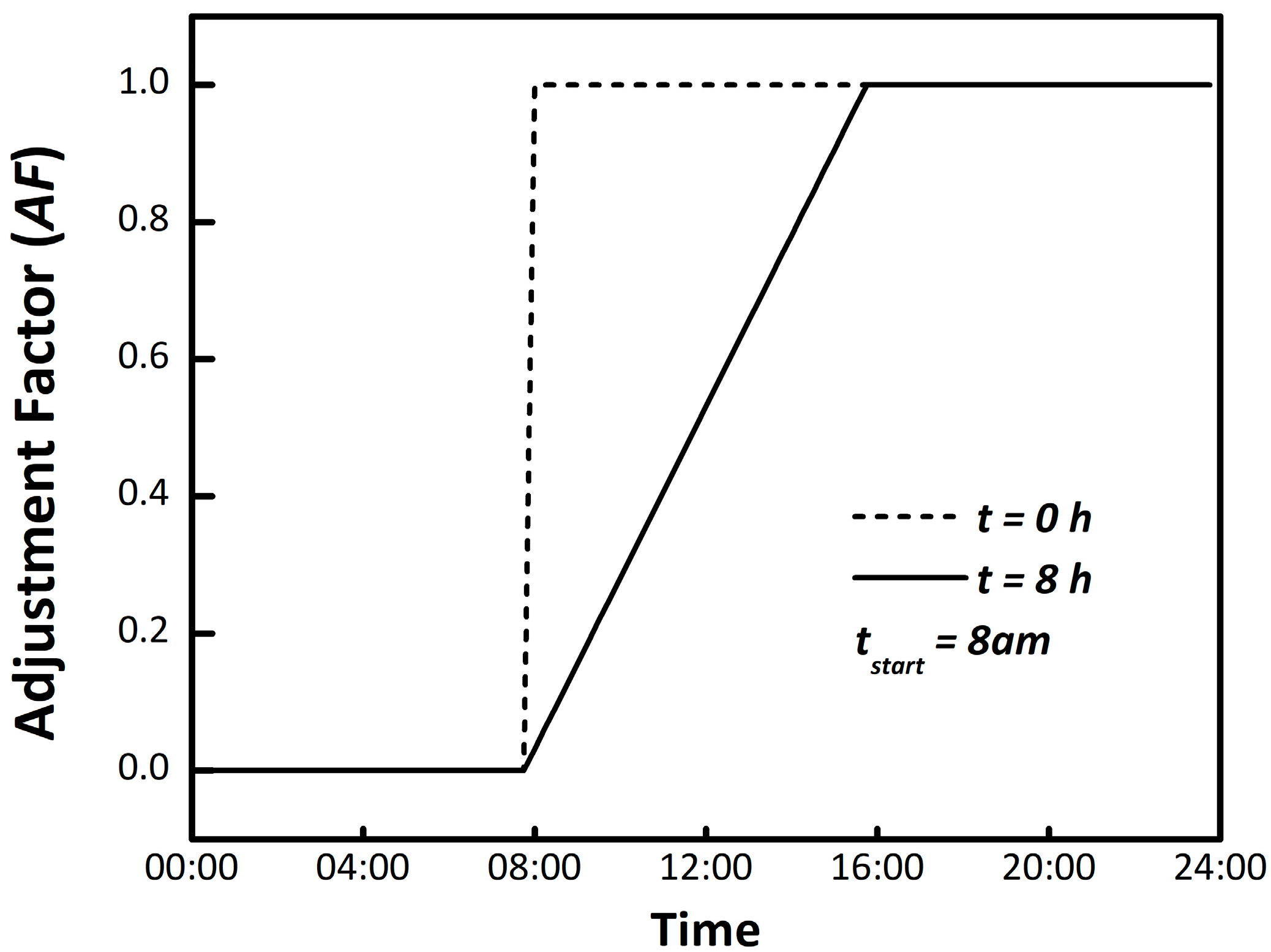
Figure 2 shows an example of how fault evolution is implemented. The time required (τ) for the fault to reach the full level is user-specified and required only if the user wants to model fault evolution. If fault evolution is not desired, τ can be set equal to zero such that the user-defined fault intensity will be imposed as a step function. However, by defining a nonzero value for τ, the fault-starting timestamp, and fault-ending timestamp, the user can enable fault evolution in the model. An adjustment factor (AF) is calculated at each time step (beginning with the starting timestamp) to gradually impose the fault intensity over the user-specified time frame, as shown in Equation (1). In this equation, AF^(t) is the adjustment factor for the fault intensity in the current time step of the simulation, calculated based on the adjustment factor from the previous time step (AF^(t−∆t)), simulation time step (∆t), and the time required for the fault to reach the full level (τ). AF^(t) is then multiplied by the user-defined fault intensity at each simulation time step. This feature is implemented via the Energy Management System object in EnergyPlus. Although at present the implementation simplifies the relationship between time and fault intensity by assuming linearity, it is possible to modify the Energy Management System code to implement nonlinearity—including discontinuous evolution where the fault intensity changes only when certain equipment is in use (direct expansion (DX) unit, fan, and so on)—if better data for understanding the fault evolution become available.

$${AF}^{\left(t\right)}={AF}^{\left(t-\mathsf{∆}t\right)}+\frac{\mathsf{∆}t}{\tau }$$

(1)

4.1. Physical Models

The physical modeling approach implements a fault by modifying existing EnergyPlus variables that directly represent physical properties. Some faults, such as building envelope infiltration, air duct leakage, oversized equipment, stuck economizer dampers, and biased economizer sensors are simulated by replacing the existing variable(s) of the associated EnergyPlus object with modified values. Faults that use the schedule object in EnergyPlus as a regular input, such as the HVAC/lighting setback and thermostat bias faults, are implemented by modifying the schedule object directly. The accuracy of estimating the fault impact with this model type depends on the thermal and mechanical dynamics of the building model itself. Thus, it is necessary to have a calibrated building model to simulate the proper impact of faults with this model type. Table 1 includes a list of 10 individual physical models considered in this study, detailed in the following subsections.

4.1.1. Excessive Infiltration Through the Building Envelope

Excessive infiltration through the building envelope from outside air typically results from cracks in the building envelope and overuse of windows and doors. Infiltration is driven by pressure differences between the building exterior and interior caused by wind and by air buoyancy forces, known commonly as the stack effect. Excessive infiltration can affect thermal comfort, indoor air quality, heating and cooling demand, and the moisture levels of building envelope components, leading to moisture damage. The infiltration through the building envelope can be modeled in EnergyPlus with varying levels of fidelity, from constant infiltration during the entire simulation period, to modulated infiltration in each time step, depending on the ambient conditions (temperature and wind speed). The fault intensity is defined as the ratio of excessive infiltration through the building envelope compared to the unfaulted condition.

4.1.2. HVAC Setback Error: Delayed Onset/Early Termination/No Overnight Setback

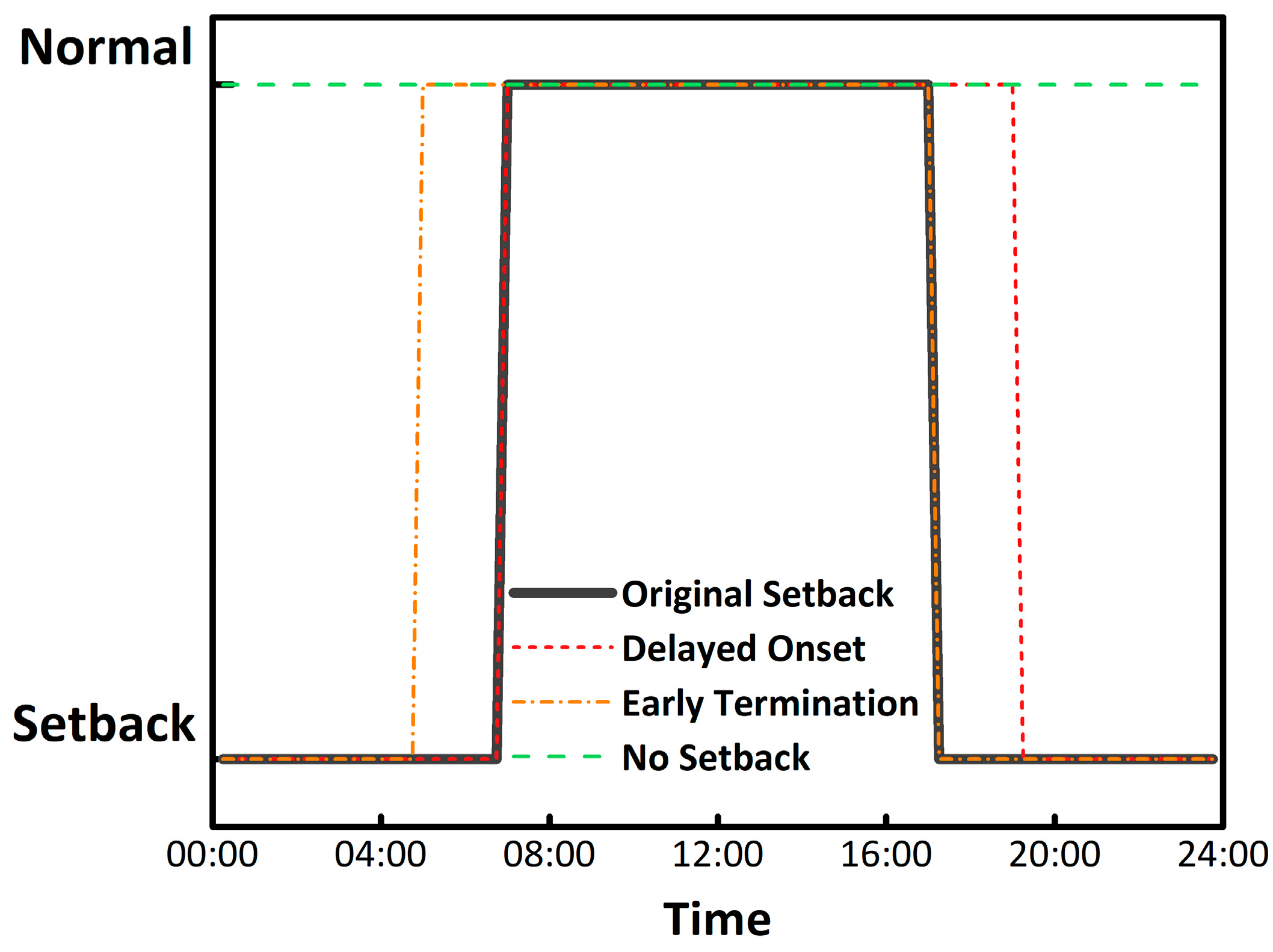
Thermostat setback schedules are employed to raise setpoints in the cooling season and lower setpoints in the heating season during unoccupied hours, to switch fan operation from being continuously on during occupied times to being coupled to cooling or heating demands at other times, and to close ventilation dampers during unoccupied periods. Faults in building control systems can occur because of malfunctioning, unprogrammed, or incorrectly programmed or scheduled thermostats, leading to increased energy consumption and/or compromised comfort and air quality. The HVAC setback error fault is further divided into three different models: delayed onset, early termination, and no overnight setback. These fault models simulate the (1) effect of overnight HVAC setback being delayed beyond the end of building occupancy at night, (2) effect of overnight HVAC setback being terminated earlier than the start of occupancy in the morning, and (3) effect when the setback is not applied in the HVAC system.

Figure 3 shows example plots of differences among setback fault types. As an example, if the onset of the setback is delayed for 2 h, the setback setpoint starts at 7 pm instead of 5 pm The definitions of the fault intensity of each model can be found in Table 1.

4.1.3. Lighting Setback Error: Delayed Onset/Early Termination/No Overnight Setback

To increase energy efficiency, lighting fixtures should be turned off or lighting levels reduced during unoccupied hours. However, schedules can be improperly configured and occupants can forget to turn off lights when vacating the building. As with an HVAC setback error (Section 4.1.2), a lighting setback error fault is divided into three models (delayed onset, early termination, and no overnight setback) and the conceptual implementation of each model is similar to the example shown in Figure 3. The definitions of the fault intensity of each model can be found in Table 1.

4.1.4. Improper Time Delay Setting in Occupancy Sensors

When a space is only intermittently occupied, use of an occupancy sensor for lighting control is more suitable than fixed scheduling. Occupancy sensing prevents spaces from being left unoccupied with lights on for long durations during the day. However, setting a time delay in the occupancy sensor is a trade-off between an occupant’s visual discomfort and energy savings. If the time delay setting is applied with a very short period, the energy savings increase. However, lights turning on and off too often increases the visual discomfort for occupants of the space. Fifteen minutes of time delay is common in real applications; however, the setting can be improperly implemented in the field. The fault intensity is defined as the delayed time setting (in hours).

4.1.5. Oversized Equipment at Design

Oversizing of heating and cooling equipment is commonly accepted in real-world applications. Some system oversizing can ensure that the highest heating and cooling demands are met, but excessive oversizing of units can lead to increased equipment cycling, reduced efficiency, and increased energy usage. This fault is implemented by increasing the capacity ratings of HVAC equipment in the model prior to executing the simulation. The fault intensity is defined as the ratio of increased sizing compared to the original sizing.

4.1.6. Supply Air Duct Leakages

Duct leakage can be caused by torn or missing external duct wrap, poor workmanship around duct takeoffs and fittings, disconnected ducts, improperly installed duct mastic, and temperature and pressure cycling. Conditioned air leaking to an unconditioned space in buildings or to the ambient space increases the equipment heating or cooling demand and can increase fan power for variable air volume (VAV) systems. The fault intensity is defined as the ratio of the leaked flow relative to the supply airflow.

4.1.7. Return Air Duct Leakages

The return duct of an air system typically operates at negative pressure, thus the leakage in the return duct (from either outdoor or unconditioned spaces) results in increased heating and cooling loads, because of unconditioned air being drawn into the return duct and mixing with the return air from conditioned spaces. The fault model simulates the return air duct leakage by modifying the amount of outdoor air introduced to the air system. The fault intensity is defined as the unconditioned outdoor air introduced to the return air stream at full load condition as a ratio of the total return airflow rate.

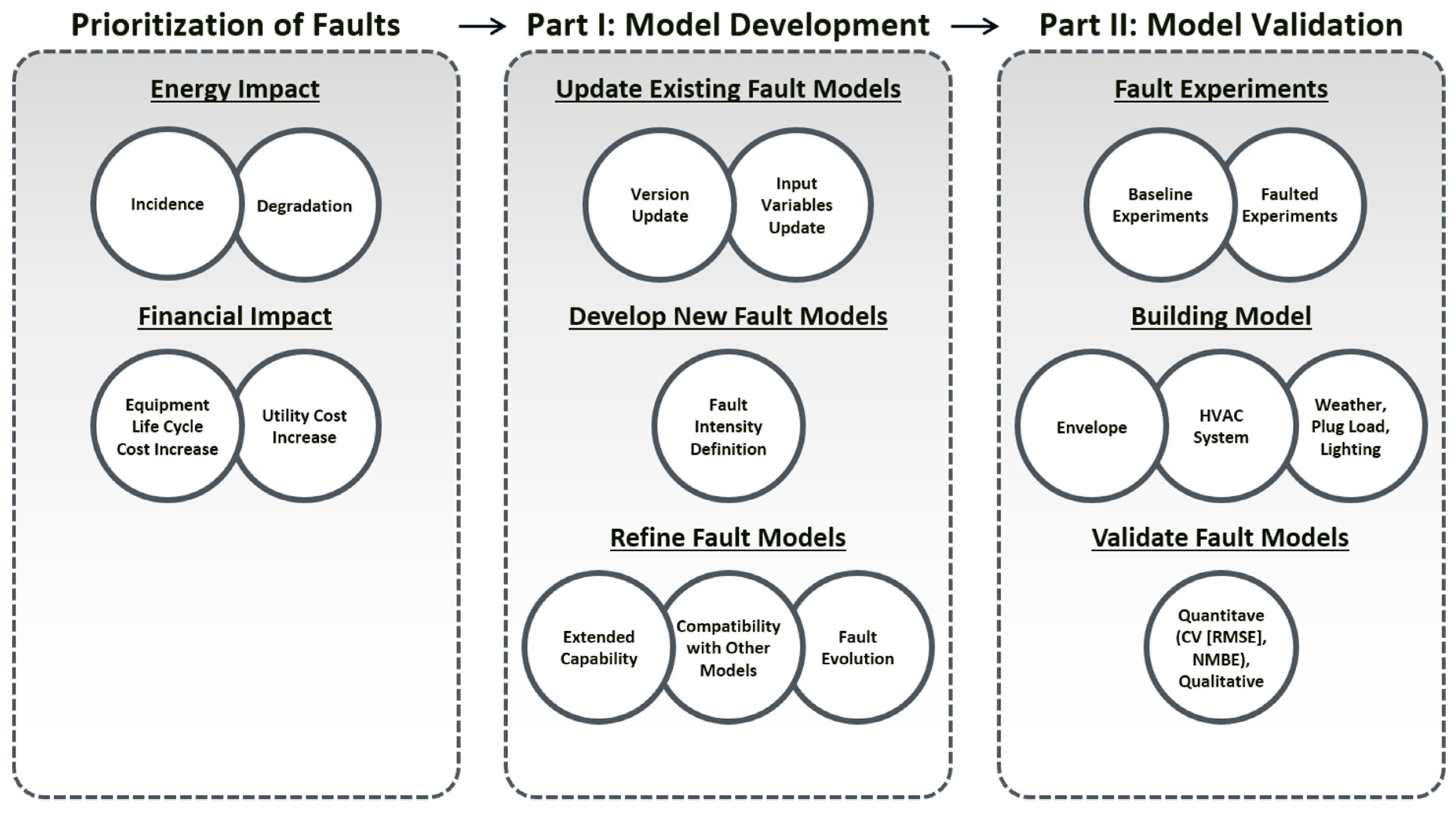
Figure 4 shows a simulation example of 48 h of system operation for this fault, including three cases: fault free operation (fault intensity (FI) = 0, τ = 0 h), faulted operation without fault evolution (FI = 0.2, τ = 0 h), and faulted operation with fault evolution (FI = 0.2, τ = 30 h). When there is a 20% (of the return airflow rate) leak at the return air duct, the fault model overrides the economizer to increase the outdoor air fraction. Then, the return air stream coming into the mixing chamber is reduced by the same amount of that addition. As shown in Figure 4, the additional fraction of the outdoor air under the unfavorable ambient condition results in additional cooling energy consumption. In the scenario with fault evolution, we observe a steady increase in the outdoor air (OA) fraction and direct expansion (DX) unit’s energy consumption until the leak stabilizes at 20% in 30 h (τ = 30 h).

4.1.8. Thermostat Measurement Bias

Drift of thermostat temperature sensors over time can lead to increased energy use and/or reduced occupant comfort. The fault model for thermostat measurement bias simulates a biased thermostat by modifying the heating and cooling setpoints assigned to thermal zones. The fault intensity is defined as the absolute thermostat measurement bias (K), where a positive number means the sensor reading is higher than the true temperature.

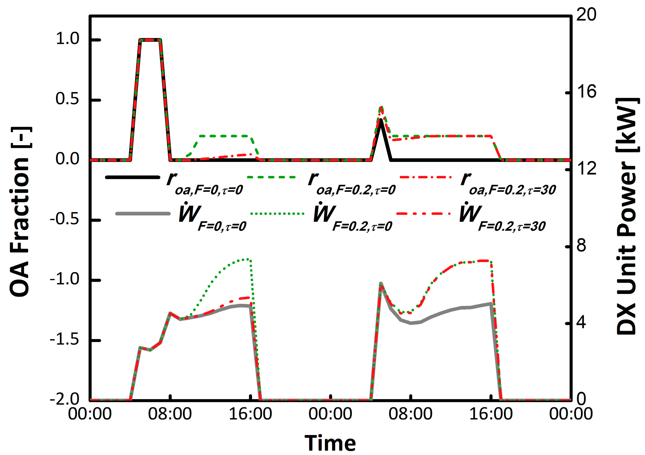
Figure 5 shows a simulation example of 48 h of system operations including three cases: fault free operation (FI = 0 K, τ = 0 h), faulted operation without fault evolution (FI = 2 K, τ = 0 h), and faulted operation with fault evolution (FI = 2 K, τ = 24 h). As shown in this figure, the fault starts at the beginning of the second day and the cooling setpoint temperature is reduced by 2 °C to mimic a condition where the sensor reads 2 °C higher than the true value. As a result, the cooling energy consumption increases in both faulted cases.

4.1.9. Economizer Opening Stuck at a Fixed Position

Stuck economizer dampers can be caused by seized actuators, broken linkages, economizer control system failures, or the failure of sensors that are used to determine the damper position. In extreme cases, dampers stuck at either 100% open or closed can have a serious impact on system energy consumption or occupant comfort in the space. This fault is implemented by overriding the economizer control algorithm to fix the damper permanently at a user-specified value. The fault intensity for this fault is defined as the stuck economizer damper position (0 = fully closed, 1 = fully open).

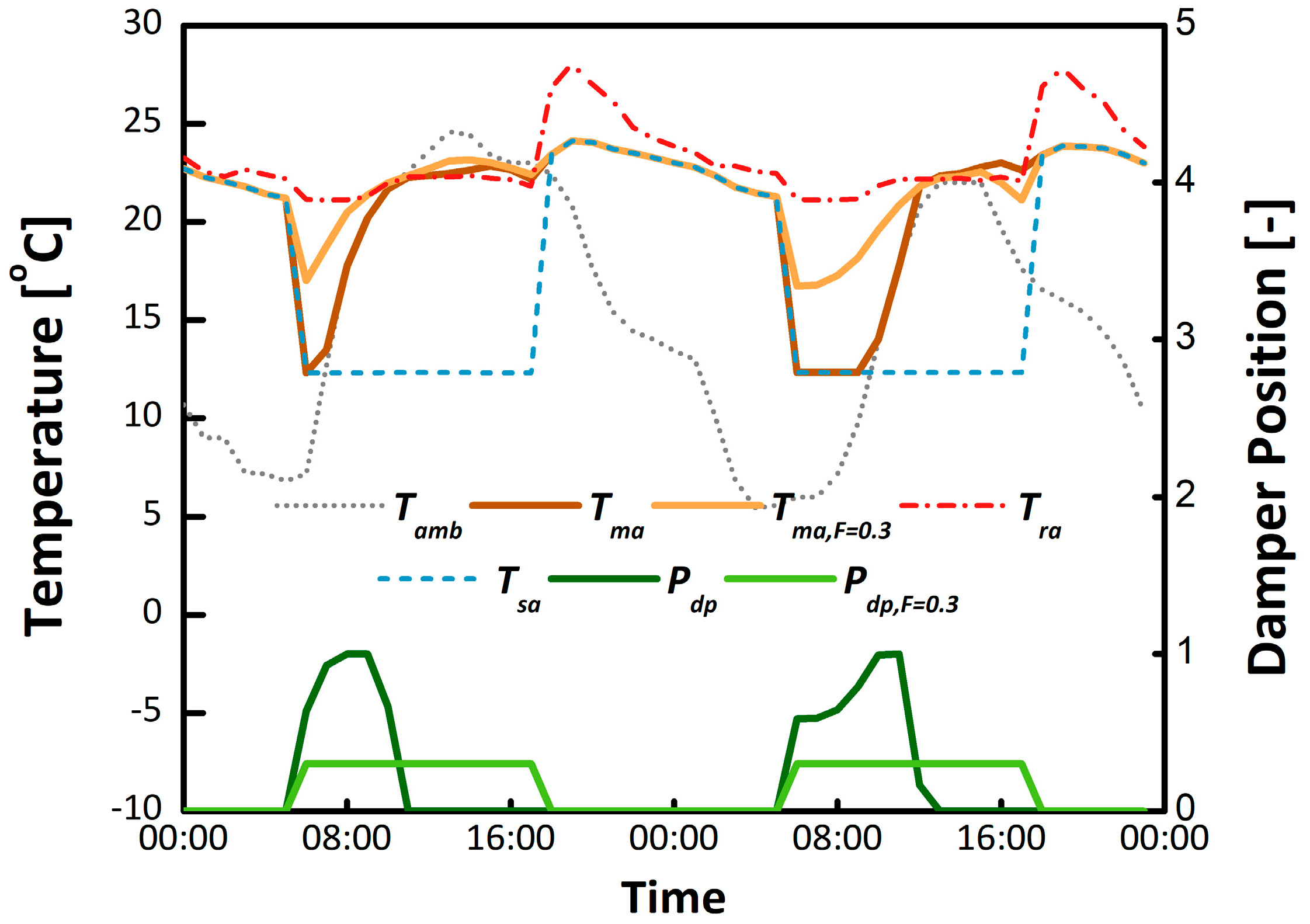
Figure 6 shows a simulation example of 48 h of economizer operations with and without the fault, in which the economizer outdoor air damper is stuck at 30% for the faulted condition. As shown in this figure, there are opportunities for free cooling during early occupied hours (around 6 am) because the outdoor temperature is below the supply air temperature setpoint. However, as temperatures rise later in the day, it becomes advantageous to close the damper. Whereas the normally operated economizer modulates the outdoor damper to set the mixed air temperature to the supply air temperature setpoint, the faulted damper position is stuck at 30%. The stuck damper results in a higher mixed-air temperature compared to the mixed-air temperature of the normally operated condition in this scenario. Because this mixed-air temperature must be cooled down to the supply air temperature setpoint, the faulted case results in additional cooling energy consumption.

4.1.10. Biased Economizer Sensors: Mixed Temperature, Outdoor Relative Humidity/Outdoor Temperature/Return Relative Humidity/Return Temperature

When a sensor drifts and is not regularly calibrated, it causes a bias. Sensor readings often drift from their calibration with age, causing equipment control algorithms to produce outputs that deviate from their intended function. The biased economizer sensor fault is divided into five different models depending on the sensor location and type: mixed temperature, outdoor relative humidity, outdoor temperature, return relative humidity, and return temperature. All the other sensor fault models modify the outside air control sequence, whereas the biased mixed air temperature sensor fault is simulated by modifying a setpoint schedule. The fault intensity is defined as the temperature offset (K), where a positive number means that the sensor reading is higher than the true temperature.

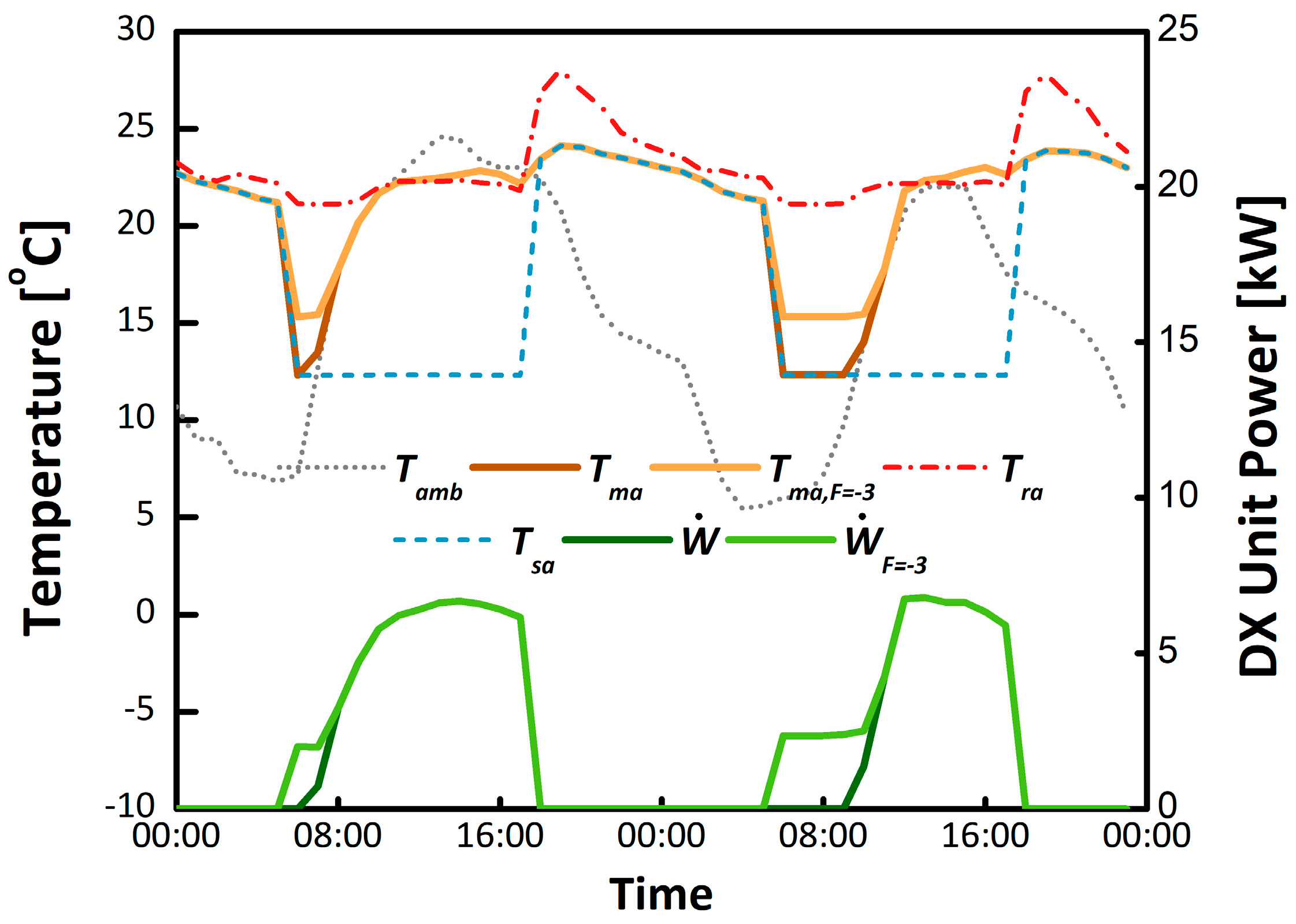
Figure 7 shows a simulation example of 48 h of operations with and without the mixed air temperature fault. As shown in the figure, the mixed air temperature setpoint is increased by 3 °C to mimic a condition where the mixed air temperature sensor reads 3 °C lower than the true value. When the outdoor condition is favorable for the free cooling (from 6 a.m. to 8 a.m. in both days), this results in additional cooling energy consumption, because the economizer is not fully taking advantage of the favorable ambient condition.

Bias faults associated with outdoor relative humidity, outdoor temperature, return relative humidity, and return temperature sensors are implemented by overriding the economizer sensor values within the economizer controller. Unlike the mixed air temperature sensor bias fault, these models calculate the amount of outdoor air based on the biased level of each sensor and replace the existing outdoor airflow rate parameter in EnergyPlus. The fault intensities of each model are defined in Table 1.

There are different economizer control strategies (e.g., fixed dry bulb, differential dry bulb, fixed enthalpy, differential enthalpy, and so on) that use different criteria and sensor sets for enabling economizing mode. The fixed control strategies use outdoor air sensor(s), and the differential control strategies use both outdoor and return air sensors. The dry-bulb control strategies only use temperature sensor(s), whereas the enthalpy control strategies use both temperature and humidity sensors to calculate enthalpy. Thus, the impact of biased sensor faults on economizer performance differs depending on the economizer control type.

4.2. Empirical Models

In this work, empirical fault models were implemented that directly modify outputs from empirical correlations used in EnergyPlus objects. This model type is useful for modeling building components that have complicated operating principles with less computational burden than would be required to represent the underlying physical behavior of the component. Faults that commonly occur in vapor compression systems are modeled with this approach; the basis of this modeling approach is adopted from Cheung and Braun [28]. For vapor compression systems, Equations (2)–(4) show empirical equations for fault impact ratios (FIR) that modify cooling capacity (${\dot{Q}}_{cool}$), energy input ratio (EIR), and evaporator heat transfer conductance (${UA}_{rat}$) as a function of user-defined fault intensity (FI), ambient temperature (T_db,amb), evaporator air inlet wet-bulb temperature (T_wb,ent), and the rated conditions for cooling capacity (${\dot{Q}}_{cool,rat}$) and power consumption (${\dot{W}}_{cool,rat}$). The coefficients for these empirical equations were determined using linear regression with the training data for each fault derived from a detailed, physics-based fault simulation. Detailed information regarding the models and training data is documented in Cheung and Braun [13,14,28]. Table 1 includes the list of four empirical models considered in this study and descriptions of each fault model are shown in the following subsections.

$$\begin{array}{cc}\hfill {FIR}_{\dot{Q}}=\frac{{\dot{Q}}_{cool,F}}{{\dot{Q}}_{cool}}& \\ & =1+FI\{c_{F,0}+c_{F,1}(\frac{T_{wb,ent}}{273.15}+1)+c_{F,2}(\frac{T_{db,amb}}{273.15}+1)+c_{F,3}FI\hfill \\ & +c_{F,4}{FI}^2+c_{F,5}\frac{{\dot{Q}}_{cool,rat}}{{\dot{W}}_{cool,rat}}\}\hfill \end{array}$$

(2)

$$\begin{array}{cc}\hfill {FIR}_{EIR}=\frac{{EIR}_F}{EIR}& \\ & =1\hfill \\ & +FI\{c_{F,6}+c_{F,7}\left(\frac{T_{wb,ent}}{273.15}+1\right)+c_{F,8}\left(\frac{T_{db,amb}}{273.15}+1\right)+c_{F.9}FI\hfill \\ & +c_{F,10}{FI}^2+c_{F,11}\frac{{\dot{Q}}_{cool,rat}}{{\dot{W}}_{cool,rat}}\}\hfill \end{array}$$

(3)

$${UA}_{rat,F}=\left(1+c_{F,12}FI\right){UA}_{rat}$$

(4)

4.2.1. Condenser Fouling

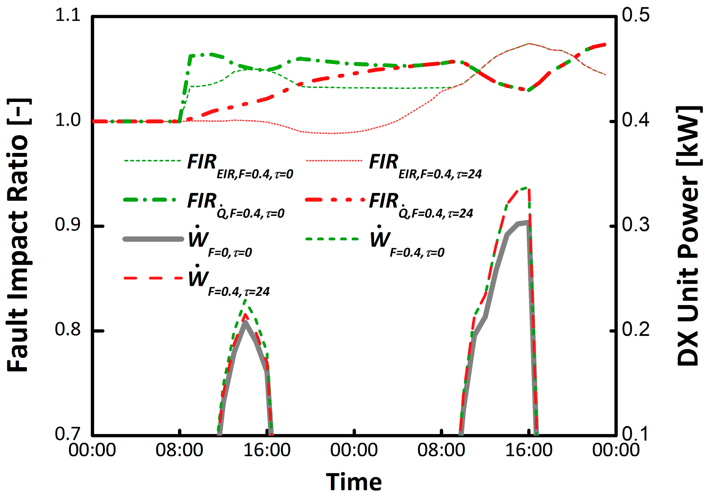
Condenser fouling occurs when litter, dirt, or dust accumulates on or between the fins of a condenser of an air conditioner. The blockage reduces the airflow across the condenser coil(s) and increases the condensing temperature in the refrigerant circuit. The elevated temperature increases the pressure difference across the compressor and reduces the equipment efficiency. This fault model captures this effect through increased power consumption and reduced total cooling capacity. Thus, ${FIR}_{\dot{Q}}$ and ${FIR}_{EIR}$ are calculated with Equations (2) and (3) in these models and are updated at each time step during the simulation, corresponding to the varying operating conditions of the DX unit. The fault intensity is defined as the ratio of reduction in condenser coil airflow at full load with an application range of 0 to 0.5 (50% reduction).

Figure 8 shows a simulation example of 48 h of DX unit operations with three different cases: fault-free operation (FI = 0, τ = 0 h), faulted operation without fault evolution (FI = 0.4, τ = 0 h) and faulted operation with fault evolution (FI = 0.4, τ = 24 h). Condenser fouling starts at 8 am on the first day. The variations in FIR depending on operating conditions are clearly observable in the figure. Because the fault evolution is applied with τ = 24 h, both ${FIR}_{\dot{Q},F=0.4,\tau =24}$ and ${FIR}_{EIR,F=0.4,\tau =24}$ reach full impact at 8 am on the second day. The changes in FIR result in additional cooling energy consumption ($\dot{\mathrm{W}}$_{F=−0.3,τ=0}, $\dot{\mathrm{W}}$_{F=−0.3,τ=24}).

4.2.2. Nonstandard Refrigerant Charging

A nonstandard refrigerant charging fault occurs when the mass of refrigerant within the refrigerant circuit of an air-conditioning, heat pump, or refrigeration system differs from the correct value. The fault may be caused by leakage (undercharge) or by improper charging during service (undercharge or overcharge). Without the proper amount of refrigerant running in the system, the average refrigerant density, the evaporating temperature, and the refrigerant mass flow rate from the compressor decrease, leading to reduced capacity, increased operating time, and increased energy consumption. Unlike the condenser fouling fault, the remaining empirical fault models also capture its effect on the evaporator heat transfer conductance using Equation (4). Thus, Equations (2)–(4) are used in these models, and, although ${FIR}_{\dot{Q}}$ and ${FIR}_{EIR}$ are updated at each time step during the simulation, the ${UA}_{rat}$ calculation is used to update the rated sensible heat ratio parameter in EnergyPlus in the beginning of the simulation. The fault intensity is defined as the ratio of charge deviation from the normal charge level with an application range of −0.3 to 0.15 (negative FI = undercharge, positive FI = overcharge).

4.2.3. Presence of Noncondensable Gas in Refrigerant

When an air conditioner, heat pump, or refrigeration unit is not properly evacuated prior to being charged with refrigerant, the unit runs with a mixture of air and refrigerant. Because air is noncondensable, any air inside the refrigerant circuit will typically become trapped in the high-pressure vapor downstream of the compressor, and the pressure difference across the compressor and the compressor power consumption increases as a result. The fault model simulates the effect of noncondensable gas by modifying performances of the total cooling capacity, energy input ratio, and sensible heat ratio using Equations (2)–(4). The fault intensity is defined as the ratio of the mass of noncondensable gas in the refrigerant circuit to the mass of noncondensable gas that the refrigerant circuit can hold at standard atmospheric pressure, with an application range of 0 to 0.6.

4.2.4. Refrigerant Liquid–Line Restriction

A liquid–line restriction fault occurs when particles accumulate within the refrigerant filter located between the condenser and the expansion valve in the refrigerant circuit of a vapor compression cycle. The accumulation increases the flow resistance within the refrigerant circuit; increases the pressure difference across the compressor; reduces the evaporating temperature; and leads to lower cooling capacity, efficiency, and sensible heat ratio. The lower sensible heat ratio leads to an increased latent load to meet a particular sensible load. The fault model simulates a liquid–line restriction by modifying performances of the total cooling capacity, energy input ratio, and sensible heat ratio using Equations (2)–(4). The fault intensity is defined as the ratio of increase in the pressure difference between the condenser outlet and evaporator inlet because of the restriction, with an application range of 0 to 0.3.

4.3. Semiempirical Models

The semiempirical modeling approach implements a fault by modifying both empirical correlations and physical properties in EnergyPlus objects. For example, the fan model in EnergyPlus uses a normalized fan curve that is based on an empirical correlation, but the relation of the fan curve to the fault impact is modeled using physical properties. The basis of these models is also adopted from the previous study of Cheung and Braun [28]. Table 1 includes the three semiempirical models considered in this study, and descriptions of each fault model are presented in the following subsections.

4.3.1. Air Handling Unit Fan Motor Degradation

Fan motor degradation occurs because of bearing and stator winding faults, leading to a decrease in motor efficiency and an increase in overall fan power consumption. The fault model simulates the air handling unit fan motor degradation by modifying the total efficiency of the fan based on the user-defined fault intensity. The fault intensity for this fault is defined as the ratio of fan motor efficiency degradation, with an application range of 0 to 0.3 (30% degradation).

4.3.2. Duct Fouling

Ducts are fouled by dust that accumulates in the filter and/or fins of heat exchangers in indoor air ducts. The accumulation increases the flow resistance of the air duct and changes the airflow through, and pressure drop across, the duct in accordance with the controls of the fan rotational speed. The fault model simulates the duct fouling by modifying the pressure rise, maximum airflow, and minimum airflow in the fan model based on the user-defined fault intensity. The fault intensity is defined as the reduction in airflow at full load condition as a ratio of the design airflow rate, with an application range of 0 to 0.5 (50% reduction).

4.3.3. Condenser Fan Degradation

Motor efficiency degrades when a motor suffers from a bearing or a stator winding fault. This fault causes the motor to draw higher electrical current without changing the fluid flow. Both a bearing fault and a stator winding fault can be modeled by increasing the power consumption of the condenser fan without changing the fan’s airflow. The fault model simulates the condenser fan degradation by modifying the energy input ratio in the DX unit model based on a user-defined fault intensity. The fault intensity is defined as the reduction in motor efficiency as a fraction of the unfaulted motor efficiency, with an application range of 0 to 0.3 (30% degradation).

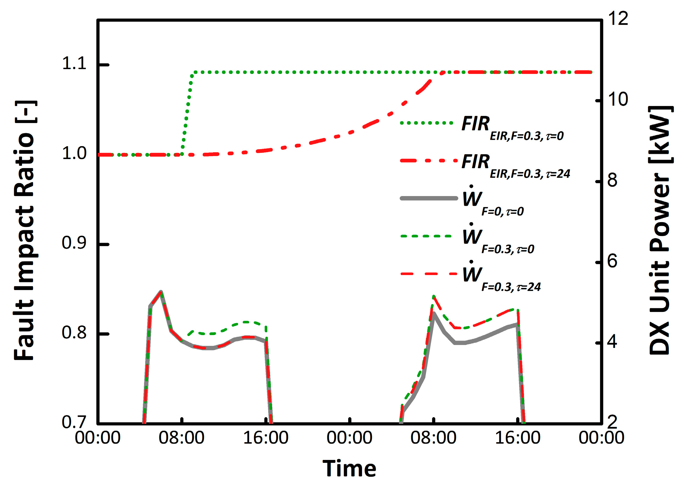
Figure 9 shows a simulation example of 48 h of DX unit operation with three different cases: fault free operation (FI = 0, τ = 0 h), faulted operation without fault evolution (FI = 0.3, τ = 0 h) and faulted operation with fault evolution (FI = 0.3, τ = 24 h). Condenser fan degradation starts at 8 am on the first day. The condenser fan degradation fault affects only condenser fan power; it has no effect on the cooling performance (total cooling capacity) of the vapor compression system. A simple equation shown in Equation (5) is used to characterize the impact on equipment efficiency (FIR_EIR) that is based on a derivation provided in Cheung and Braun [28]. For the case without fault evolution, the fault impact ratio for EIR (FIR_EIR,F=0.3) is calculated with Equation (5) and is applied to the conversion from the cooling capacity to power consumption in each time step. For the case with fault evolution, the fault impact ratio (FIR_{EIR,F=0.3,τ=24}) is also calculated with Equation (5), but fault intensity (FI) is now affected by the adjustment factor at every time step, and FIR_{EIR,F=0.3,τ=24} gradually increases to reach the full level in 24 h. These changes in FIR result in additional cooling energy consumption ($\dot{W}$_{F=−0.3,τ=0}, $\dot{W}$_{F=−0.3, τ=24}).

$${FIR}_{EIR}=\frac{{FIR}_F}{EIR}=1+\frac{{\dot{W}}_{fan}}{{\dot{W}}_{cool}}\left(\frac{FI}{1-FI}\right)$$

(5)

5. Case Study: Generating a Training Data Set

An accurate building model combined with fault models can be used to generate large volumes of diverse training data for data-driven FDD algorithm development. As mentioned in Section 1, generating a training data set via simulation has advantages over acquiring the same data set from field measurements: the ground truth is known with certainty; the cost of generating evaluation samples is low; evaluation samples can be generated for a wide variety of equipment, building types, environmental conditions, and so on; and evaluation data sets may be constructed without significant gaps or biases [10,12].

This section presents a case study generating an FDD training data set with EnergyPlus that includes all the faults described in Table 1. The results shown in this section demonstrate the capability to generate fault impact data using physics-based building model combined with fault models, that could ultimately be used in the development and evaluation of automated fault detection and diagnosis (AFDD) algorithms. More detailed results, which are used as a basis for prioritizing sensors, are included in the Supplementary Material section.

5.1. Characteristics of the Reference Building Model

An existing building was used as a basis to develop the building model; this building is research-oriented and represents a typical light commercial office building that has the capability to emulate actual building behaviors such as occupancy, lighting load, plug load, and HVAC operation.

Table 2. Characteristics of the Reference Building Model.

Building Type	Office
Weather data (location)	Knoxville, TN (TMY3)
Building total floor area	297 m2
Building width, length, and height	12.2 × 12.2 × 4.3 m
Number of floors	2
Number of thermal zones	10 (8 perimeter and 2 core)
Building envelope	Wall structure: Concrete masonry units with face brick Wall insulation: Fiberglas RUS-11 (Btu/(h-F-ft2)/RSI-1.9 (W/m-K) Floor: Slab-on-grade Roof structure: Metal deck with polyisocyanurate and ethylene proplylene diene monomer Roof insulation: Polyisocyanurate RUS-18/RSI-3.17 Windows: Aluminum frame, double-pane, clear glazing Window-to-wall ratio: 28%
HVAC system	Rooftop unit: DX unit (12.5 ton, EER 9.6), Furnace (natural gas fired, AFUE 81%) Variable air volume system (electric reheat coil)
Plug load	Lighting power density: 0.85 W/ft2 (9.2 W/m2) with lighting on/off schedule Equipment power density: 1.3 W/ft2 (14.0 W/m2) with on/off schedule

summarizes the building characteristics. Im et al. [35] and Goldwasser et al. [36] describe the development and calibration of the EnergyPlus model of this building used in the present work.

5.2. Generation of the Training Data Set

Physics-based building models developed in EnergyPlus and OpenStudio provide extensive model outputs (equivalent to sensor measurements in actual buildings) that capture detailed building behavior and performance. When a fault occurs in the building, a subset of these outputs is affected, with the exact subset dependent on the nature of the fault. However, not all of the model outputs are always available in actual buildings. Because building automation systems and their sensors have associated capital and operating costs, installers may not include many sensors—or even an automation system—in an actual building. Thus, finding the minimum set of sensors that is effective for detecting and diagnosing various faults in small commercial buildings is a key strategy for developing cost-effective, data-driven AFDD algorithms. Knowledge of the minimum sensors required for effective AFDD enables optimization of the sensor suite and increases the average value delivered by each installed sensor.

We generated a curated fault model simulation data set (the data set is publicly available [37]) that consists of tagged and fully described time series representing simulated faults for the reference building (described in Section 5.1), including both baseline (unfaulted) performance and faulted performance. 25 faults were simulated at various fault intensity levels for a total of 99 simulation scenarios. Each simulation scenario was simulated for a year with a time resolution of 15 min. For all faulted scenarios, only one fault was applied for each scenario; multiple faults in one scenario were not considered in the training data set. Fault evolution was not considered either, because of the sparsity of accurate information for selecting appropriate parameters that model the evolution of various faults.

5.3. Prioritization of Sensors Affected by Faults

To verify and prioritize sensors that are affected by each fault, we compared the model outputs from the baseline (unfaulted) simulation scenario against the same outputs in each faulted scenario. For each output, we calculated the normalized mean bias error (NMBE) of the faulted measurement compared to the baseline measurement for each output using Equation (6), where $n$ is the total number of datapoints in each simulation scenario (equal to 8760 × 4 = 35,040), $y_B$ is the value of the output in the baseline scenario, $y_F$ is the value of the output in the faulted scenario, and ${\overline{y}}_B$ is the average of the entire $y_{B,i}$ at each time step i. NMBE represents the relative deviation from the baseline measurement, including the sign convention (the direction in which the fault is affecting the measurement), and is used to quantify the impact of the fault on each sensor.

$$NMBE=\frac{1}{{\overline{y}}_B}\frac{{\sum }_{i=1}^n\left(\frac{y_{F,i}-y_{B,i}}{y_{B,i}}\right)}{n}$$

(6)

Table 3. List of Sensors Considered for Prioritization.

Sensor Name	Sensor Availability	Sensor Category
Building electricity	Basic	Building
Zone temp	Basic	Zone
RTU cooling coil air outlet temp	Moderate	RTU
RTU heating coil air outlet temp	Moderate	RTU
RTU mixed air temp	Moderate	RTU
RTU supply air temp	Moderate	RTU
Submeter: HVAC	Moderate	Submeter
Zone relative humidity	Moderate	Zone
RTU cooling coil capacity	Rich	RTU
RTU cooling coil runtime fraction	Rich	RTU
RTU economizer status	Rich	RTU
RTU fan airflow rate	Rich	RTU
RTU fan power	Rich	RTU
RTU heating coil capacity	Rich	RTU
RTU heating coil runtime fraction	Rich	RTU
RTU outdoor air fraction	Rich	RTU
Submeter: cooling	Rich	Submeter
Submeter: heating (elec)	Rich	Submeter
Submeter: heating (gas)	Rich	Submeter
Submeter: lighting	Rich	Submeter
VAV reheat air outlet temp	Rich	VAV box
VAV reheat coil capacity	Rich	VAV box

lists the model outputs (sensors) for which NMBE values were calculated. Each sensor shown in the table is also classified by typical availability category and sensor category. Three availability categories are used: the “basic” sensor set includes sensors that are typically available even without a building automation system; the “moderate” sensor set represents sensors that are commonly available in typical building automation systems; and the “rich” sensor set represents sensors that are physically plausible but not included in either the basic or moderate sensor sets. The sensor category represents the general purpose or function of the sensor: building level meter, building submeter, zone sensors, RTU sensors, or VAV box sensors. Detailed NMBE calculations for each sensor and fault that were used as a basis for prioritizing sensors affected by each fault are included in Figures S1–S16 in Supplementary Materials.

Based on results from Figures S1–S16, Tables S1–S3 (in Supplementary Materials) summarize the top five sensors prioritized, based on the NMBEs that were calculated for each fault for heating season (January–February), cooling season (July–August), and shoulder season (April–May), respectively, for the considered weather conditions. In summary, the prioritized sensors change by the season for faults that directly affect both heating and cooling season operations (e.g., HVAC setback error, thermostat bias, air duct leakages, and excessive infiltration). In the heating season, preheating- and reheating-related sensors (e.g., RTU heating coil capacity, RTU heating coil runtime, submeter: heating [gas], submeter: heating [elec], and VAV reheat coil capacity) become dominant in the prioritized lists. Cooling- and reheating-related sensors (e.g., RTU cooling coil capacity, submeter: cooling, submeter: heating [elect]) become dominant in the cooling season. Faults that affect specific equipment (e.g., fan motor degradation, faults in the vapor compression system, and faults in lighting system) do not significantly change in the list of prioritized sensors between seasons. Further discussions of Tables S1–S3 are also included in the Supplementary Material section.

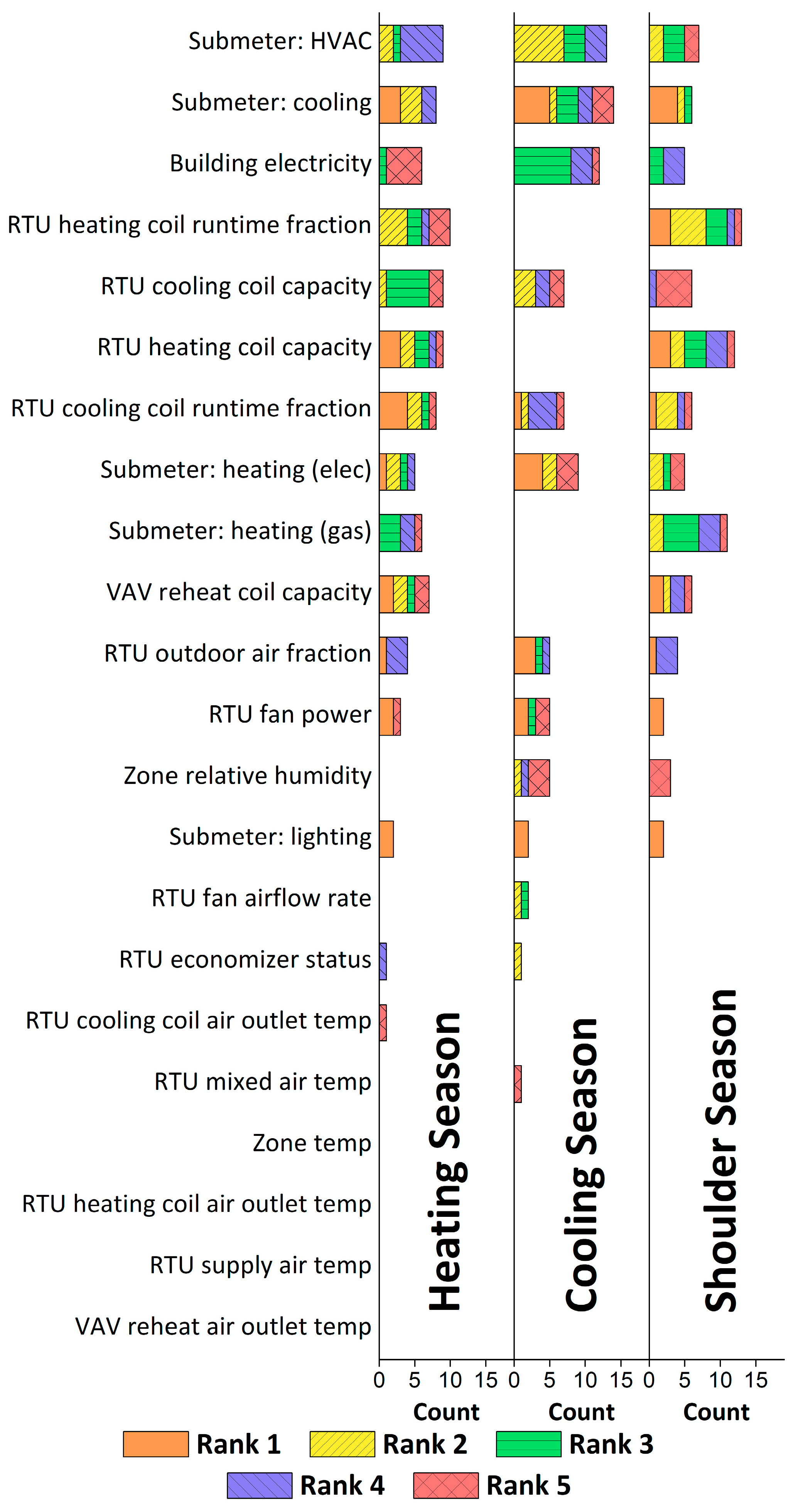
Figure 10 shows an overall prioritized sensors list, that was obtained by counting the number of each sensor shown in Tables S1–S3. The order of the ranked list is based on the total count of heating, cooling, and shoulder season results. Figure 10 also includes additional detail on the rank of the sensors between 1st and 5th, shown in Tables S1–S3.

The Submeter: the HVAC sensor showed the highest count for all seasons and for all considered faults, because it includes fault impacts from the heating, cooling, and ventilation (fan) subsystems. Submeter: cooling was the second most counted sensor; it is affected by all faults in the vapor compression system. The whole-building electricity measurement (building electricity sensor in the figure) is ranked third overall in frequency, even though it was never selected as one of the first two sensors in the prioritized lists of Tables S1–S3. As expected, the heating-related sensors (e.g., RTU heating coil runtime, RTU heating coil capacity, submeter: heating [gas], and VAV reheat coil capacity) were rarely included in the cooling season’s prioritized sensors list, as shown in the cooling season column in Figure 10. Measurements of the zone air temperatures and temperatures in the RTU (e.g., fan outlet, heating coil outlet, supply air, and VAV reheat coil outlet) were never indicated as prioritized sensors for any faults or season.

Figure 10 illustrates relative impacts between sensors for all faults described in Section 4. Although the prioritized sensors shown in this figure are specific to a particular building located in Knoxville, Tennessee, the results demonstrate insights that can be gained from fault modeling, that are relevant for developing and training a case-specific AFDD algorithm.

6. Conclusions

This work was motivated by development of a cost-effective AFDD tool for the small commercial buildings market, where the energy savings potential is high but the return of AFDD tool investment is low. The focus of the overall research was to develop a cost-effective, model-based AFDD tool that uses building energy simulation software (EnergyPlus and OpenStudio). The tool leverages fault models to generate an AFDD algorithm training data set.

This paper is Part I of a two-part sequence that describes the development and validation of models for faults common in small commercial buildings. This article introduced the development of a library of fault models, including detailed descriptions for the implementation of each fault. Additionally, it presented a case study for generating a training data set that represents an actual building, in which impacts on the building model outputs (equivalent to building sensors) were studied to understand how fault signatures are reflected in a training data set. Although the fault models introduced covered the scope of this study, there are limitations in these models that require future work: limited compatibility against existing objects in EnergyPlus, incapability of simulating multiple faults in the same simulation scenario, incapability of coupling specific building operations with the fault evolution model, and limited focus on only small commercial buildings, whilst other various faults (faults in larger building systems; boiler, chiller, cooling tower, etc.) are not covered. Part II describes an experimental validation methodology used for a subset of the developed fault models and validation results.